https://doi.org/10.5194/npg-25-355-2018 © Author(s) 2018. This work is distributed under the Creative Commons Attribution 4.0 License.
Feature-based data assimilation in geophysics
Matthias Morzfeld, Jesse Adams, Spencer Lunderman, and Rafael Orozco
Department of Mathematics, University of Arizona, 617 N. Santa Rita Ave., P.O. Box 210089, Tucson, Arizona 85721, USA Correspondence:Matthias Morzfeld ([email protected])
Received: 14 September 2017 – Discussion started: 6 October 2017
Revised: 30 January 2018 – Accepted: 10 April 2018 – Published: 3 May 2018
Abstract.Many applications in science require that compu-tational models and data be combined. In a Bayesian frame-work, this is usually done by defining likelihoods based on the mismatch of model outputs and data. However, match-ing model outputs and data in this way can be unnecessary or impossible. For example, using large amounts of steady state data is unnecessary because these data are redundant. It is numerically difficult to assimilate data in chaotic systems. It is often impossible to assimilate data of a complex system into a low-dimensional model. As a specific example, con-sider a low-dimensional stochastic model for the dipole of the Earth’s magnetic field, while other field components are ignored in the model. The above issues can be addressed by selecting features of the data, and defining likelihoods based on the features, rather than by the usual mismatch of model output and data. Our goal is to contribute to a fundamental understanding of such a feature-based approach that allows us to assimilate selected aspects of data into models. We also explain how the feature-based approach can be interpreted as a method for reducing an effective dimension and derive new noise models, based on perturbed observations, that lead to computationally efficient solutions. Numerical implementa-tions of our ideas are illustrated in four examples.
Copyright statement. The author’s copyright for this publication is transferred to the United States Government. The United States Government retains and the publisher, by accepting the article for publication, acknowledges that the United States Government re-tains a nonexclusive, paid-up, irrevocable, worldwide license to publish or reproduce the published form of this paper, or allow oth-ers to do so, for United States Government purposes. The U.S. De-partment of Energy will provide public access to these results of federally sponsored research in accordance with the DOE Public
Access Plan (http://energy.gov/downloads/doe-public-access-plan; last access: 20 April 2018).
1 Introduction
The basic idea of data assimilation is to update a com-putational model with information from sparse and noisy data so that the updated model can be used for predictions. Data assimilation is at the core of computational geophysics, e.g., in numerical weather prediction (Bauer et al., 2015), oceanography (Bocquet et al., 2010) and geomagnetism (Fournier et al., 2010). Data assimilation is also used in en-gineering applications, e.g., in robotics (Thrun et al., 2005) and reservoir modeling (Oliver et al., 2008). We use the term “data assimilation” broadly, but focus on parameter estima-tion problems where one attempts to find model parame-ters such that the output of the model matches data. This is achieved by defining a posterior distribution that describes the probabilities of model parameters conditioned on the data.
modeling of the Earth’s dipole for timescales of millions of years as discussed, e.g., in Gissinger (2012), Petrelis et al. (2009), Buffett et al. (2013), and Buffett and Matsui (2015). These simplified models cannot represent all aspects of the Earth’s magnetic field and, hence, using observations of the Earth’s magnetic field for parameter or state estimation with these models is not possible. We will elaborate on this exam-ple in Sect. 4.3. Another examexam-ple of low-dimensional models for complex processes are the simplified delay-differential equations used by Koren and Feingold (2011), Feingold and Koren (2013), and Koren et al. (2017), to model behaviors of cloud systems over warm oceans. In both cases, model out-puts cannot directly match data, because the low-dimensional model was not designed to capture all aspects of a com-plex system (clouds or the Earth’s dipole). Second, matching model outputs to data directly becomes numerically impossi-ble if one considers chaotic models over long timescales. We will discuss this case in detail in Sect. 4.4.
The above issues can be addressed by adapting ideas from machine learning to data assimilation. Machine learn-ing algorithms expand the data into a suitable basis of “fea-ture vectors” (Murphy, 2012; Bishop, 2006; Rasmussen and Williams, 2006). A feature can be thought of as a low-dimensional representation of the data, e.g., a principal com-ponent analysis (PCA) (Jolliffe, 2014), a Gaussian process (GP) model (Rasmussen and Williams, 2006), or a Gaus-sian mixture model (McLachlan and Peel, 2000). Features are either constructed a priori, or learned from data. The same ideas carry over to data assimilation. One can extract low-dimensional features from the data and use the model to reproduce these features. A feature-based likelihood can be constructed to measure the mismatch of the observed fea-tures and the feafea-tures produced by the model. The based likelihood and a prior distribution define a feature-based posterior distribution, which describes the probability of model parameters conditioned on the features. We mostly discuss features that are constructed a priori and using phys-ical insight into the problem. Learning features “automati-cally” from data is the subject of future work.
As a specific example, consider a viscously damped har-monic oscillator, defined by damping and stiffness coeffi-cients (we assume we know its mass). An experiment may be to pull on the mass and then to release it and to measure the displacement of the mass from equilibrium as a function of time. These data can be compressed into features in var-ious ways. For example, a feature could be the statement that “the system exhibits oscillations”. Based on this fea-ture, one can infer that the damping coefficient is less than 1. Other features may be the decay rate or observed oscilla-tion frequency. One can compute the damping and stiffness coefficients using classical formulas, if these quantities were known exactly. The idea of feature-based data assimilation is to make such inferences in view of uncertainties associated with the features.
Another example is Lagrangian data assimilation for fluid flow, where the data are trajectories of tracers and where a natural candidate for a feature is a coherent structure (Maclean et al., 2017). The coherent structure can be used to formulate a likelihood, which in turn defines a posterior dis-tribution that describes the probability of model parameters given the observed coherent structure, but without direct ap-peal to tracer trajectories. More generally, consider a chaotic system observed over long timescales, e.g., severale-folding times of the system. Due to the chaotic behavior, changes in the numerical differential equation solver may change like-lihoods based on model-output–data mismatch, even if the parameters and data remain unchanged. The feature-based approach can be useful here, as shown by Hakkarainen et al. (2012), who use likelihoods based on particle filter runs to average out uncertainties from differential equation solvers. Haario et al. (2015) use correlation vectors and summary statistics, which are “features” in our terminology, to identify parameters of chaotic systems such as the Lorenz 63 (Lorenz, 1963) and Lorenz 95 (Lorenz, 1995) equations.
Our goal is to contribute to a fundamental understanding of the feature-based approach to data assimilation and to ex-tend the numerical framework for solving feature-based data assimilation problems. We also discuss the conditions un-der which the feature-based approach is appropriate. In this context, we distinguish two problem classes. First, the com-pression of the data into a feature may lead to no or little loss of information, in which case the feature-based prob-lem and the “original” probprob-lem, as well as their solutions, are similar. Specific examples are intrinsically low-dimensional data or redundant (steady state) data. Second, the features extracted from the data may be designed to deliberately ne-glect information in the data. This second case is more in-teresting because we can assimilate selected aspects of data into low-dimensional models for complex systems and we can formulate feature-based problems that lead to useful pa-rameter estimates for chaotic systems, for which a direct ap-proach is computationally expensive or infeasible. We give interpretations of these ideas in terms of effective dimensions of data assimilation problems (Chorin and Morzfeld, 2013; Agapiou et al., 2017) and interpret the feature-based ap-proach as a method for reducing the effective dimension. Our discussion and numerical examples suggest that the feature-based approach is comparable to a direct approach when the data can be compressed without loss of information and that computational efficiency is gained only when the features truly reduce the dimension of the data, i.e., if some aspects of the data are indeed ignored.
numer-ical methods for data assimilation, e.g., Monte Carlo sam-pling or optimization. We suggest overcoming this difficulty by adapting ideas from stochastic ensemble Kalman filters (Evensen, 2006) and to derive noise models directly for the features using “perturbed observations”. Such noise models lead to feature-based likelihoods which are easy to evaluate, so that Monte Carlo methods can be used for the solution of feature-based data assimilation problems. Another numeri-cal difficulty is that the feature-based likelihood can be noisy, e.g., if it is based on averages computed by Monte Carlo sim-ulations. In such cases, we suggest applying numerical opti-mization to obtain maximum a posteriori estimates, rather than Monte Carlo methods, because optimization is more ro-bust to noise.
Details of the numerical solution of feature-based data assimilation problems are discussed in the context of four examples, two of which involve “real” data. Each exam-ple represents its own challenges and we suggest appropri-ate numerical techniques, including Markov Chain Monte Carlo (MCMC; Kalos and Whitlock, 1986), direct sampling (see, e.g., Chorin and Hald, 2013; Owen, 2013) and global Bayesian optimization (see, e.g., Frazier and Wang, 2016). The variety of applications and the variety of numerical methods we can use to solve these problems indicate the flex-ibility and usefulness of the feature-based approach.
Ideas related to ours were recently discussed by Rosen-thal et al. (2017) in the context of data assimilation problems in which certain geometric features need to be preserved. This situation occurs, e.g., when estimating wave character-istics, or tracking large-scale structures such as storm sys-tems. Data assimilation typically does not preserve geomet-ric features, but Rosenthal et al. (2017) use kinematically constrained transformations to preserve geometric features within an ensemble Kalman filtering framework. The tech-niques discussed by Rosenthal et al. (2017) are related to the feature-based data assimilation we describe here, but they differ at their core and their goals: Rosenthal et al. (2017) are concerned aboutpreservingfeatures during data assimilation while we wish toestimatemodel parameters from features. We further emphasize that a feature-based approach may also be useful when high-fidelity models, such as coupled ocean– hurricane models, are used. In this case, one may need to reduce the dimension of some of the data and assimilate only some features into the high-dimensional model. This is dis-cussed in Falkovich et al. (2005) and Yablonsky and Ginis (2008). Here, we focus on problems in which the data are high-dimensional, but the model is low-dimensional.
2 Background
We briefly review the typical data assimilation problem for-mulation and several methods for its numerical solution. The descriptions of the numerical techniques may not be suffi-cient to fully comprehend the advantages or disadvantages
of each method, but these are explained in the references we cite.
2.1 Data assimilation problem formulation
Suppose you have a mathematical or computational model Mthat maps input parametersθto outputsy, i.e.,y=M(θ)
whereθandyaren- andk-dimensional real vectors. The pa-rametersθmay be initial or boundary conditions of a partial differential equation, diffusion coefficients in elliptic equa-tions, or growth rates in ecological models. The outputsy can be compared to dataz, obtained by observing the physi-cal process under study. For example, ifMis an atmospheric model,zmay represent temperature measurements atk dif-ferent locations. It is common to assume that
z=M(θ)+ε, (1)
whereεis a random variable with known probability density functionpε(·)that describes errors or mismatches between
model and data. The above equation defines ak-dimensional “likelihood”, l(z|θ)=pε(z−M(θ)|θ), that describes the
probability of the data for a given set of parameters.
In addition to Eq. (1), one may have prior information about the model parameters, e.g., one may know that some parameters are nonnegative. Such prior information can be represented by a prior distributionp0(θ). By Bayes’ rule, the
prior and likelihood define the posterior distribution
p(θ|z)∝p0(θ) l(z|θ). (2)
The posterior distribution combines information from model and data and defines parametersθthat lead to model outputs that are “compatible” with the data. Here compatible means that model outputs are likely to be within the assumed errors ε.
Data assimilation problems of this kind appear in sci-ence and engineering, e.g., in numerical weather prediction, oceanography and geomagnetism (Bocquet et al., 2010; van Leeuwen, 2009; Fournier et al., 2010), as well as in global seismic inversion (Bui-Thanh et al., 2013), reservoir mod-eling or subsurface flow (Oliver et al., 2008), target track-ing (Doucet et al., 2001), and robotics (Thrun et al., 2005; Morzfeld, 2015). The term “data assimilation” is common in geophysics, but in various applications and disciplines, different names are used, including parameter estimation, Bayesian inverse problems, history matching and particle fil-tering.
2.2 Numerical methods for data assimilation
as is the case in numerical weather prediction. The second group consists of optimization algorithms, called “variational methods” in this context (Talagrand and Courtier, 1987). The third group are Monte Carlo sampling methods, includ-ing particle filters or direct samplinclud-ing (Owen, 2013; Doucet et al., 2001; Atkins et al., 2013; Morzfeld et al., 2015), and MCMC (Mackay, 1998; Kalos and Whitlock, 1986). We will use variational methods, MCMC and direct sampling for nu-merical solution of feature-based data assimilation problems and we briefly review these techniques here.
In variational data assimilation one finds the parameter set θ∗ that maximizes the posterior probability, which is also called the posterior mode. One can find the posterior mode by minimizing the negative logarithm of the posterior distri-bution
F (θ)= −log(p0(θ) l(z|θ)) . (3)
The optimization is done numerically and one can use, for example, Gauss–Newton algorithms. In some of the numer-ical examples below, we need to optimize functions F (θ)
that are computationally expensive to evaluate and noisy, i.e.,
F (θ)is a random variable with unknown distribution. The source of noise in the function F (θ)is caused by numeri-cally approximating the feature. Suppose, e.g., that the fea-ture is an expected value and in the numerical implemen-tation this expected value is approximated by Monte Carlo. The Monte Carlo approximation, however, depends on the number of samples used and if this number is small (finite), the approximation is noisy, i.e., the Monte Carlo average for the same set of parameters θ, but with two different seeds in the random number generator, can lead to two different values forF (θ). In such cases, one can use a derivative free optimization method such as global Bayesian optimization (GBO); see, e.g., Frazier and Wang (2016). The basic idea is to model the function F (θ) by a Gaussian process and then update the GP model based on a small number of func-tion evaluafunc-tions. The points where the funcfunc-tion is evaluated are chosen based on an expected improvement (EI) criterion, which takes into account where the function is unknown or known. The GP model for the functionF (θ)is then updated based on the function evaluations at the points suggested by EI. One can iterate this procedure and when the iteration is finished, e.g., because a maximum number of function eval-uations is reached, one can use the optimizer of the mean of the GP model to approximate the optimizer of the (random) functionF (θ).
In MCMC, a Markov chain is generated by drawing a new sample θ0 given a previous sampleθj−1, using a proposal distributionq(θ0|θj−1). The proposed sampleθ0is accepted asθj or rejected based on the values of the posterior distri-bution of the new and previous samples; see, e.g., Mackay (1998) and Kalos and Whitlock (1986). Averages over the samples converge to expected values with respect to the pos-terior distribution as the number of samples goes to infinity.
However, sinceθj depends onθj−1, the samples are not in-dependent and one may wonder how many effectively un-correlated samples one has obtained. This number can be estimated by dividing the number of samples by the inte-grated auto-correlation time (IACT) (Mackay, 1998; Kalos and Whitlock, 1986). Thus, one wants to pick a proposal distribution that reduces IACT. The various MCMC algo-rithms in the literature differ in how the proposal distribu-tion is constructed. In the numerical examples below, we use the MATLAB implementation of the affine invariant en-semble sampler (Goodman and Weare, 2010), as described by Grinsted (2017), and we use the numerical methods de-scribed in Wolff (2004) to compute IACT.
In direct sampling (sometimes called importance sam-pling) one generates independent samples using a proposal densityqand attaches to each sample a weight:
θj∼q(θ), wj∝p0(θ
j) l(z|θj)
q(θj) .
Weighted averages of the samples converge to expectations with respect to the posterior distribution as the number of samples goes to infinity. While the samples are independent, they are not all equally weighted and one may wonder how many “effectively unweighted” samples one has. For an en-semble of sizeNe, the effective number of samples can be
estimated as (Doucet et al., 2001; Arulampalam et al., 2002)
Neff=Ne/ρ, ρ= E(w2)
E(w)2. (4)
For a practical algorithm, we thus choose a proposal distri-butionqsuch thatρis near 1. There are several strategies for constructing such proposal distributions and in the numerical illustrations below we use “implicit sampling” (Chorin and Tu, 2009; Morzfeld et al., 2015; Chorin et al., 2016) and con-struct the proposal distribution to be a Gaussian whose mean is the posterior modeθ∗and whose covariance is the Hessian ofF in Eq. (3), evaluated atθ∗(see also Owen, 2013).
3 Feature-based data assimilation
The basic idea of feature-based data assimilation is to replace the data assimilation problem defined by a priorp0(θ)and
the likelihood in Eq. (1) by another problem that uses only selected features of the dataz. We assume that the prior is appropriate and focus on constructing new likelihoods. Let F(·) be anm-dimensional vector function that takes a k -dimensional data set into am-dimensional feature. One can apply the feature-extraction to Eq. (1) and obtain
f=F(M(θ)+ε) , (5)
lF(f|θ), which in turn defines a feature-based posterior
dis-tribution,pF(θ|f)∝p0(θ) lF(f|θ). The feature-based
pos-terior distribution describes the probabilities of model pa-rameters conditioned on the feature f and can be used to make inferences about the parametersθ.
3.1 Noise modeling
Evaluating the feature-based posterior distribution is diffi-cult because evaluating the feature-based likelihood is cum-bersome. Even under simplifying assumptions of additive Gaussian noise in Eq. (1), the likelihood lF(f|θ), defined
by Eq. (5), is generally not known. The reason is that the feature functionF makes the distribution ofF(M(θ)+ε)
non-Gaussian even ifεis Gaussian. Numerical methods for data assimilation typically require that the posterior distribu-tion be known up to a multiplicative constant. This is gen-erally not the case when a feature-based likelihood is used (the feature-based likelihood is Gaussian only ifFis linear and ifεis Gaussian). Thus, variational methods, MCMC or direct sampling are not directly applicable to solve feature-based data assimilation problems defined by Eq. (5). More advanced techniques, such as approximate Bayesian compu-tation (ABC) (Marin et al., 2012), however, can be used be-cause these are designed for problems with unknown likeli-hood (see Maclean et al., 2017).
Difficulties with evaluating the feature-based likelihood arise because we assume that Eq. (1) is accurate and we re-quire that the feature-based likelihood follows directly from it. However, in many situations the assumptions about the noise ε in Eq. (1) are “ad hoc”, or for mathematical and computational convenience. There is often no physical rea-son why the noise should be additive or Gaussian, yet these assumptions have become standard in many data assimilation applications. This leads to the question:why not “invent” a suitable and convenient noise model for the feature?
We explore this idea and consider an additive Gaussian noise model for the feature. This amounts to replacing Eq. (5) by
f =MF(θ)+η, (6)
whereMF =F◦M, is the composition of the model M
and feature extractionF, andηis a random variable that rep-resents uncertainty in the feature and which we need to de-fine (see below). For a givenη, the feature-based likelihood defined by Eq. (6), lF(f|θ)=pη(f−MF(θ)|θ), is now
straightforward to evaluate (up to a multiplicative constant) because the distribution ofηis known or chosen. The feature-based likelihood feature-based on Eq. (6) results in the feature-feature-based posterior distribution
pF(θ|f)∝p0(θ) lF(f|θ), (7)
wherep0(θ)is the prior distribution, which is not affected
by defining or using features. The usual numerical tools, e.g.,
MCMC, direct sampling, or variational methods, are applica-ble to the feature-based posterior distribution (Eq. 7).
Our simplified approach requires that one defines the dis-tribution of the errors η, similar to how one must specify the distribution ofεin Eq. (1). We suggest using a Gaus-sian distribution with mean zero forη. The covariance that defines the Gaussian can be obtained by borrowing ideas from the ensemble Kalman filter (EnKF). In a “perturbed observation” implementation of the EnKF, the analysis en-semble is formed by using artificial perturbations of the data (Evensen, 2006). We suggest using a similar approach here. Assuming that ε in Eq. (1) is Gaussian with mean 0 and covariance matrixR, we generate perturbed data by zj∼N(z,R),j =1, . . ., N
z. Each perturbed datum leads to
a perturbed featurefj=F(zj)and we compute the
covari-ance Rf =
1
Nz−1
Nz
X
j=1
(fj−f)(fj−f)T.
We then use η∼N(0,Rf) as our noise model for the
feature-based problem in Eq. (6).
Note that the rank of the covariance Rf is
min{dim(f ), Nz−1}. For high-dimensional features,
the rank ofRf may therefore be limited by the number of
perturbed observations and features we generate, and this number depends on the computational requirements of the feature extraction. We assume that Nz is larger than the
dimension of the feature, which is the case if either the computations to extract the features are straightforward, or the feature is low-dimensional.
One may also question whyηshould be Gaussian. In the same vein, one may wonder whyεin Eq. (1) should be Gaus-sian, which is routinely assumed. We do not claim that we have answers to such questions, but we speculate that if the feature does indeed constrain some parameters, then assum-ing a unimodal likelihood is appropriate and, in this case, a Gaussian assumption is also appropriate.
3.2 Feature selection
Feature-based data assimilation requires that one defines and selects relevant features. In principle, much of the machine learning technology can be applied to extract generic fea-tures from data. For example, one can defineFby the PCA, or singular value decomposition, of the data and then neglect small singular values and associated singular vectors. As a specific example, suppose that the data are measurements of a time series ofMdata points of ann-dimensional system. In this case, the functionMF consists of the following steps:
Lagrangian data assimilation, coherent structures (and their SVDs) are a natural candidate, as explained by Maclean et al. (2017). In Sect. 4 we present several examples of “intuitive” features, constructed using physical insight, and discuss what numerical methods to use in the various situations.
The choice of the feature suggests the numerical meth-ods for the solution of the feature-based problem. One is-sue here is that, even with our simplifying assumption of ad-ditive (Gaussian) noise in the feature, evaluating a feature-based likelihood can be noisy. This happens in particular when the feature is defined in terms of averages over solu-tions of stochastic or chaotic equasolu-tions. Due to limited com-putational budgets, such averages are computed using a small sample size. Thus, sampling error is large and evaluation of a feature-based likelihood is noisy, i.e., evaluations of the feature-based likelihood, even for the same set of parameters θand feature-dataf, may lead to different results, depending on the state of the random number generator. This additional uncertainty makes it difficult to solve some feature-based problems numerically by Monte Carlo. However, one can construct a numerical framework for computing maximum a posteriori estimates using derivative-free optimization meth-ods that are robust to noise, e.g., global Bayesian optimiza-tion (Frazier and Wang, 2016). We will specify these ideas in the context of a numerical example with the Kuramoto– Sivashinsky (KS) equation in Sect. 4.4.
3.3 When is a feature-based approach useful?
A natural question is the following: under what conditions should I consider a feature-based approach? There are three scenarios which we discuss separately before we make con-nections between the three scenarios using the concept of “effective dimension”.
3.3.1 Case (i): data compressionwithoutinformation loss
It may be possible that data can be compressed into features without significant loss of information, for example, if obser-vations are collected while a system is in steady state. Steady state data are redundant, make negligible contributions to the likelihood and posterior distributions and, therefore, can be ignored. This suggests that features can be based on truncated data and that the resulting parameter estimates and posterior distributions are almost identical to the estimates and poste-rior distributions based onallthe data. We provide a detailed numerical example to illustrate this case in Sect. 4.1. Simi-larly, suppose the feature is based on the PCA of the data, e.g., only the firstd singular values and associated singular vectors are used. If the neglected singular values are indeed small, then the data assimilation problem defined by the fea-ture, i.e., the truncated PCA, and the data assimilation prob-lem defined by all of the data, i.e., the full set of singular val-ues and singular vectors, are essentially the same. We discuss
this in more detail and with the help of a numerical example in Sect. 4.2.
3.3.2 Case (ii): data compressionwithinformation loss
In some applications a posterior distribution defined by all of the data may not be practical or computable. An exam-ple is estimation of initial conditions and other parameters based on (noisy) observations of a chaotic system over long timescales. In a “direct” approach one tries to estimate initial conditions that lead to trajectories that are near the observa-tions at all times. Due to the sensitivity to initial condiobserva-tions a point-wise match of model output and data is numerically difficult to achieve. In a feature-based approach one does not insist on a point-by-point match of model output and data, i.e., the feature-based approach simplifies the problem by neglecting several important aspects of the data during the feature-extraction (e.g., the time-ordering of the data points). As a specific example consider estimation of model parame-ters that lead to trajectories with similar characteristics to the observed trajectories. If only some characteristics of the tra-jectories are of interest, then the initial conditions need never be estimated. Using features thus avoids the main difficulty of this problem (extreme sensitivity to small perturbations) provided one can design and extract features that are robust across the attractor. Several examples have already been re-ported where this is indeed the case; see Hakkarainen et al. (2012), Haario et al. (2015), and Maclean et al. (2017). We will provide another example and additional explanations, in particular about feature selection and numerical issues, in Sect. 4.4. It is important to realize that thesolution of the feature-based problem is different from the solution of the (unsolvable) original problem because several important as-pects of the data are ignored. In particular, we emphasize that the solution of the feature-based problem yields parameters that lead to trajectories with similarities with the data, as de-fined by the feature. The solution of the (possibly infeasible) original problem yields model parameters that lead to trajec-tories that exhibit a good point-by-point match with the data. 3.3.3 Case (iii): models and data at different scales
the feature-based approach may be useful in this context. We discuss this case in more detail and with the help of a numer-ical example in Sect. 4.3.
3.3.4 Reduction of effective dimension
Cases (i) and (ii) can be understood more formally using the concept of an “effective dimension”. The basic idea is that a high-dimensional data assimilation problem is more difficult than a low-dimensional problem. However, it is not only the number of parameters that defines dimension in this context, but rather a combination of the number of parameters, the assumed distributions of errors and prior probability, as well as the number of data points (Chorin and Morzfeld, 2013; Agapiou et al., 2017). An effective dimension describes this difficulty of a data assimilation problem, taking into account all of the above, and is focused on the computational require-ments of numerical methods (Monte Carlo) to solve a given problem: a low effective dimension means the computations required to solve the problem are moderate. Following Aga-piou et al. (2017) and assuming a Gaussian prior distribution,
p0(θ)=N(µ,P), an effective dimension is defined by
efd=Tr(P− ˆP)P−1,
where Pˆ is the posterior covariance and where Tr(A)= Pn
j=1ajj is the trace of ann×nmatrixAwith diagonal
el-ementsajj,j =1, . . ., n. Thus, the effective dimension
mea-sures the difficulty of a data assimilation problem by the dif-ferences between prior and posterior covariance. This means that the more information the data contains about the param-eters, the higher is the problem’s effective dimension and, thus, the harder is it to find the solution of the data assimi-lation problem. We emphasize that this is a statement about expected computational requirements and that it is counterin-tuitive – parameters that are well-constrained by data should be easier to find than parameters that are mildly constrained by the data. However, in terms of computing or sampling pos-terior distributions, a high impact of data on parameter esti-mates makes the problem harder. Consider an extreme case where the data have no influence on parameter estimates. Then the posterior distribution is equal to the prior distri-bution and, thus, already known (no computations needed). If the data are very informative, the posterior distribution will be different from the prior distribution. For example, the prior may be “wide”, i.e., not much is known about the pa-rameters, while the posterior distribution is “tight”, i.e., un-certainty in the parameters is small after the data are col-lected. Finding and sampling this posterior distribution re-quires significantly more (computational) effort than sam-pling the prior distribution.
Case (i) above is characterized by features that do not change (significantly) the posterior distribution and, hence, the features do not alter the effective dimension of the prob-lem. It follows that the computed solutions and the required
computational cost of the feature-based or “direct” approach are comparable. In case (ii), however, using the feature rather than the data themselves indeed changes the problem and its solution, i.e., the feature-based posteriorpF(θ)can be a very
different function than the full posteriorp(θ). For example, the dimension of the feature may be lower than the dimen-sion of the full data set because several important aspects of the data are ignored by the feature. The low dimensionality of the feature also implies that the effective dimension of the problem is lower. For chaotic systems, this reduction in ef-fective dimension can be so dramatic that the original prob-lem is infeasible, while a feature-based approach becomes feasible; see Hakkarainen et al. (2012), Haario et al. (2015), Maclean et al. (2017) and Sect. 4.4.
4 Numerical illustrations
We illustrate the above ideas with four numerical examples. In the examples, we also discuss appropriate numerical tech-niques for solving feature-based data assimilation problems. The first example illustrates that contributions from redun-dant data are negligible. The second example uses “real data” and a predator–prey model to illustrate the use of a PCA fea-ture. Examples 1 and 2 are simple enough to solve by “clas-sical” data assimilation, matching model outputs and data directly and serve as an illustration of problems of type (i) in Sect. 3.3. Example 3 uses a low-dimensional model for a complex system, namely the Earth’s geomagnetic dipole field over the past 150 Myr. Here, a direct approach is in-feasible, because the model and data are describing different timescales and, thus, this example illustrates a problem of type (iii) (see Sect. 3.3). Example 4 involves a chaotic partial differential equation (PDE) and parameter estimation is diffi-cult using the direct approach because it requires estimating initial conditions. We design a robust feature that enables es-timation of a parameter of the PDE without estimating initial conditions. The perturbed observation noise models for the features are successful in examples 1–3 and we use Monte Carlo for numerical solution of the feature-based problems. The perturbed observation method fails in example 4, which is also characterized by a noisy feature-based likelihood, and we describe a different numerical approach using maximum a posteriori estimates.
ap-proach and build priors informed by previous assimilations, as is typical in sequential data assimilation.
4.1 Example 1: more data is not always better
We illustrate that a data assimilation problem with fewer data points can be as useful as one with significantly more, but redundant, data points. We consider a mass–spring–damper system
d2x
dt2 +2ζ ω
dx
dt +ω
2x=h(t−5),
wheret≥0 is time,ζ >0 is a viscous damping coefficient,
ω >0 is a natural frequency andh(τ )is the “step-function”, i.e., h(τ )=0 forτ <0 and h(τ )=1 forτ ≥0. The initial conditions of the mass–spring–damper system arex(0)=0, dx/dt (0)=0. The parameters we want to estimate are the damping coefficientζ and the natural frequencyω, i.e.,θ= (ζ, ω)T. To estimate these parameters we use a uniform prior distribution over the box [0.5,4]×[0.5,4] and measure the displacement x(t )every1t=0.5 time units (starting with a measurement at t=0). The duration of a (synthetic) ex-periment isτ=M1t and we consider experiments of dura-tions betweenτ =25 toτ =250 time units, withM=51 to
M=501 data points. The data of an experiment of duration
τ =M1tare thus
zi=x(i1t )+vi, vi∼N(0,10−3), i=0, . . ., M.
Writingz= {z0, . . ., zM}, we obtain the likelihood
lτ(z|θ)∝exp −
1 2
M
X
i=0
103(zi−x(i1T ))2
! .
The likelihood and the uniform prior distribution define the posterior distribution
pτ(θ|z)=
1
Cτ
lτ(z|θ) if θ∈[0.5,4]×[0.5,4],
0 otherwise,
where Cτ is a normalization constant. Data of an
experi-ment of durationτ=40 is shown in Fig. 1a. These synthetic data are generated with “true” parametersζ =1.5 andω=1. With these parameters the oscillator is “overdamped” and reaches its steady state (limt→∞x(t )=1) quickly. We
antic-ipate that data collected aftert≈25 is redundant in the sense that the same displacement is measured again and again. This suggests that the posterior distributions of experiments of du-rationτ=i1tandτ=j 1tare approximately equal to each other, provided thati, j >50/1t. In other words, a data as-similation problem with M=101 orM=251 data points may have “roughly the same” posterior distribution and, con-sequently, lead to similar estimates.
We investigate this idea by solving data assimilation problems with experiment durations between τ=25 and
τ=225. We compare the resulting posterior distributions
p25, . . ., p225 to the posterior distributionp250,
correspond-ing to an experiment of duration τ =250. We use the Kullback–Leibler (KL) divergence, DKL(pˆ0|| ˆp1) of two
distributions to measure “how far” two distributions are from one another. For two k-dimensional Gaussians p0=
N(m0,P0)andp1=N(m1,P1), the KL divergence is given
by
DKL(p0||p1)=
1 2
Tr(P−11P0)+(m1−m0)TP−11(m1
−m0)−k+log
detP
1
detP0 .
Note thatDKL(p0||p1)=0 if the two distributions are
identi-cal and a largeDKL(p0||p1)suggest thatp0andp1are quite
different. Computing the KL divergence for non-Gaussian distributions is numerically more challenging and here were are content to measure the distance of two distributions by the KL divergence of their Gaussian approximations. We thus compute Gaussian approximations to the posterior distribu-tionsp25, . . ., p250, by computing the posterior modeθ∗(by
Gauss–Newton optimization) and the HessianHof the neg-ative logarithm of the posterior distribution at the mode. We then define the Gaussian approximation by
pτ(θ|zM)≈ ˆpτ(θ|zM)=N(θ∗, H−1), (8)
and useDKL(pˆ250|| ˆpτ)to measure the distance ofp250 and pτ.
Each experiment is in itself a random event because the measurement noise is random. The KL divergence between the various posterior distributions is, thus, also random and we address this issue by performing 1000 independent ex-periments and then average the KL divergences. Our results are shown in Fig. 1b. We plot the average KL divergence, as well as “error bars” based on the standard deviation, as a function of the experiment duration and note an exponen-tial decrease of KL divergence with experiment duration or, equivalently, number of data points used for parameter es-timation. Thus, as we increase the number of data points, the posterior distributions get closer, as measured by this KL divergence, to the posterior distribution withM=501 data points. In other words, we obtain very similar posterior dis-tributions withM=101 orM=501 data points. This indi-cates that the steady state data can be ignored because there is little additional information in these data. These results sug-gest that the data can be compressed without significant loss of information about the parameters. One could, for exam-ple, define a feature by simply neglecting data collected after
t >30. This feature would lead to parameter estimates al-most identical to those obtained using the full data set.
Time Time
ω
ζ ζ
ω
ω
ζ
x
(t
)
x
(t
)
0 10 20 30 40 -0.2
0 0.2 0.4 0.6 0.8 1 1.2
0 10 20 30 40 -0.2
0 0.2 0.4 0.6 0.8 1 1.2
(a)
(b)
(c)
(d)
(e)
(f)
(g)
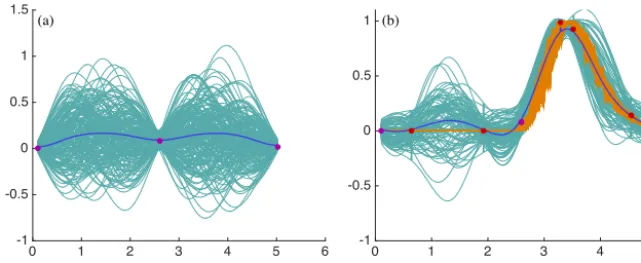
Figure 1. (a)Datazi,i=0, . . .,80 (blue dots) of an experiment of durationτ=40 and 50 trajectories of oscillators with damping coefficient
and natural frequency drawn from the posterior distributionp(θ|z)(turquoise).(b)KL divergence of approximate posterior distributions DKL(pˆ250|| ˆpτ),M=25, . . .,225, as a function of the durationτ of an experiment. Blue dots – average KL divergence of 1000
experi-ments. Red line – exponential fit. Light blue cloud: confidence interval based on standard deviations observed during the 1000 experiexperi-ments.
(c)Same data as in panel(a)(blue dots) and 50 trajectories of oscillators with damping coefficient and natural frequency drawn from the feature-based posterior distribution.(d)Histogram of the marginalp40(ζ|z0, . . ., z80)of the posterior distributionp40(θ|z0, . . ., z80)
(pur-ple) and histogram of the marginalpF(ξ|f)of the feature-based posterior distributionpF(θ|f)(blue).(e)Two-dimensional histogram of
the posterior distributionp40(θ|z0, . . ., z80).(f)Two-dimensional histogram of the feature-based posterior distributionpF(θ|f).(g)
His-togram of the marginalp40(ω|z0, . . ., z80)of the posterior distributionp40(θ|z0, . . ., z80)(purple) and histogram the marginalpF(ω|f)of
the feature-based posterior distributionpF(θ|f)(blue).
to the natural frequency since limt→∞x(t )=1/ω2. The
sec-ond component of the features is the slope of a linear fit to the seven data points collected aftert=5, i.e., after the step is applied.
The covariance matrixRof the assumed Gaussian noise η(see Eq. 6) is obtained using the perturbed observation ap-proach as described in Sect. 3.1. We generate 103perturbed data sets to compute R and find that the off-diagonal ele-ments are small compared to the diagonal eleele-ments. We thus neglect the correlation between the two components of the feature, but this is not essential. Altogether the feature-based likelihood is given by
lF(f|θ)∝exp
−1
2(f−FM(θ))
TR−1(f−F
M(θ))
,
where FM represents the following two computations:
(i) simulate the oscillator with parametersθforτ time units, and (ii) compute the feature, i.e., the average steady state value and slope, as described above. Together with the uni-form prior distribution, we obtain the feature-based posterior distribution
pF(θ|f)=
1
CF
lF(f|θ) if θ∈[0.5,4]×[0.5,4],
0 otherwise,
whereCF is a normalization constant.
We solve this feature-based problem for an experiment of durationτ =40 by implicit sampling (see Sect. 2.2) us-ingNe=103samples. From these samples we computeρ≈
posterior distribution. We note that the trajectories are all “near” the data points. For comparison, we also solve the data assimilation problem without using features and com-putep40(see Eq. 8), also by implicit sampling withNe=103
samples. We find that ρ≈1.38 in this case. We note that the feature-based posterior distribution is different from the “classical” one. This can be seen by comparing the clouds of trajectories in Fig. 1a and c. The wider cloud of trajectories indicates that the feature does not constrain the parameters as much as the full data set. The relaxation induced by the based approach, however, also results in the feature-based approach being slightly more effective in terms of the number of effective samples.
Finally, we show triangle plots of the posterior distribution
p40 and the feature-based posterior distribution in Fig. 1d–
g. A triangle plot of the feature-based posterior distribu-tion pF consists of histograms of the marginals pF(ζ|f)
and pF(ω|f), plotted in blue in Fig. 1d and e, and a
his-togram ofpF(θ|f)in Fig. 1(f). A triangle plot of the
pos-terior distribution p40(θ|z0, . . ., z80) is shown in Fig. 1d,
e and f. Specifically, we plot histograms of the marginals
p40(ζ|z0, . . ., z80)andp40(ω|z0, . . ., z80)in purple in Fig. 1d
and g and we plot a histogram of the posterior distribu-tionp40(θ|z0, . . ., z80)in Fig. 1e. We find that the marginals pF(ω|f)andp40(ω|z0, . . ., z80)are nearly identical, which
indicates that the feature constrains the frequencyω nearly as well as the full data set. The damping coefficient ζ is less tightly constrained by our feature, which results in a wider posterior distributionpF(ζ|f)thanp40(ζ|z0, . . ., z80).
A more sophisticated feature that describes the transient be-havior in more detail would lead to different results, but our main point is to show that even our simple feature, which ne-glects most of the data, leads to useful parameter estimates. 4.2 Example 2: predator–prey dynamics of lynx and
hares
We consider the Lotka–Volterra (LV) equations (Lotka, 1926; Volterra, 1926)
dx
dt =αx−βxy,
dy
dt = −γ y+δxy,
wheret is time,α, β, γ , δ >0 are parameters, andx andy
describe “prey” and “predator” populations. Our goal is to estimate the four parameters in the above equations as well as the initial conditionsx0=x(0),y0=y(0), i.e., the parameter
vector we consider isθ=(α, β, γ , δ, x0, y0)T. Since we do
not have prior information about the parameters, we choose a uniform prior distribution over the six-dimensional cube [0,10]6.
We use the lynx and hare data of the Hudson’s Bay Com-pany (Gilpin, 1973; Leigh, 1968) to define a likelihood. The data set covers a period from 1897 to 1935, with one data point per year. Each data point is a number of lynx furs and hare furs, with the understanding that the number of collected
furs is an indicator for the overall lynx or hare population. We use data from 1917 to 1927, because the solution of the LV equations is restricted to cycles of fixed amplitude and the data during this time period roughly has that quality. We scale the data to units of “104 hare furs” and “103lynx furs” (so that all numbers are order one). We use this classical data set here, but predator–prey models have recently also been used in low-dimensional cloud models that can represent certain aspects of large eddy simulations (Koren and Feingold, 2011; Feingold and Koren, 2013; Koren et al., 2017). However, the sole purpose of this example is to demonstrate that the feature-based approach is robust enough for use with “real” data (rather than the synthetic data used in example 1).
We define a featuref by the first (largest) singular value and the first left and right singular vectors of the data. The feature vector f thus has dimension 14 (we have 2×11 raw data points). We compute the noiseη for the feature-based likelihood using the “perturbed observation” method as above. We generate 10 000 perturbed data sets by adding realizations of a Gaussian random variable with mean of zero and unit covariance to the data. The resulting sample covari-ance matrix serves as the matrix Rf in the feature-based
likelihood. Note that our choice of noise on the “raw” data is somewhat arbitrary. However, as stated above, the main purpose of this example is to demonstrate our ideas, not to research interactions of lynx and hare populations.
We use the MATLAB implementation of the affine invari-ant ensemble sampler to solve the feature-based data assimi-lation problem; see Grinsted (2017) and Goodman and Weare (2010). We use an ensemble sizeNe=12 and each
ensem-ble member produces a chain of lengthns=8334. We thus
haveN=100 008 samples. Each chain is initialized as fol-lows: we first find the posterior mode using Gauss–Newton optimization. To do so, we perform an optimization with dif-ferent starting points and then choose the optimization re-sult that leads to the largest feature-based posterior proba-bility. The initial values for our ensemble of walkers are 12 draws from a Gaussian distribution whose mean is the pos-terior mode and whose covariance is a diagonal matrix with elements (0.02,0.02,0.02,0.02,0.2,0.2). We disregard the first 2500 steps of each chain as “burn-in” and compute an average IACT of 735, using the methods described in Wolff (2004). We have also performed experiments with larger en-sembles (Ne=12 is the minimum ensemble size for this
method), and with different initializations of the chains, and obtained similar results. We have also experimented with the overall number of samples (we used up to 106samples) and obtained similar results.
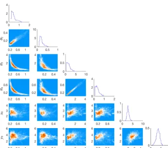
We show a triangle plot of the feature-based posterior distribution, consisting of histograms of all one- and two-dimensional marginals, in Fig. 2.
pa-θ1 θ2 θ3 θ4 x0 y0 θ2
θ3
θ4
x0
y0
Figure 2.Triangle plot of histograms of all one- and two-dimensional marginals of the feature-based posterior distribution.
rameters define the solution of the differential equation (after nondimensionalization). Perhaps most importantly, we find that the feature-based posterior distribution constraints the parameters well, especially compared to the prior distribu-tion which is a hyper-cube with sides of length 10.
We plot the trajectories of the LV equations corresponding to 100 samples of the feature-based posterior distribution in Fig. 3.
We note that the trajectories pass near the 22 original data points (shown as orange dots in Fig. 3). The fit of the lynx population is particularly good, but the trajectories of the hare populations do not fit the data well. For example, all model trajectories bend downwards towards the end of the cycle, but the data seem to exhibit an upward tendency. How-ever, this inconsistency is not due to the feature-based ap-proach. In fact, we obtain similar solutions with a “classical” problem formulation. The inconsistency is due to the limita-tions of the LV model, which is limited to cycles, whereas the data are not cyclic. Nonetheless, our main point here is that the feature-based approach is sufficiently robust that it can handle “real” data and “simple” models. We also empha-size that this data assimilation problem is not difficult to do using the “classical” approach, i.e., without using features. This suggests that this problem is of category (i) in Sect. 3.3.
H
are
L
ynx
(a)
(b)
Figure 3.Raw data (orange dots), trajectories corresponding to the feature-based posterior mode (red) and 100 trajectories of hares (turquoise) in panel(a)and lynx (blue) in panel(b), correspond-ing to 100 samples of the feature-based posterior distribution.
4.3 Example 3: variations in the Earth’s dipole’s reversal rates
re--100 -90 -80 -70 -60 -50 -40 -30 -20 -10 0 -1
0 1
-100 -90 -80 -70 -60 -50 -40 -30 -20 -10 0
-1 0 1
Time (Myr)
-100 -90 -80 -70 -60 -50 -40 -30 -20 -10 0
-1 0 1
B13
Geomagnetic polarity timescale
P09
P
ol
ari
ty a
nd
si
gne
d di
pol
e i
nt
ens
it
y
P
ol
ari
ty (a)
(b)
(c)
Figure 4. (a)The Earth’s dipole polarity over the past 100 Myr (part of the geomagnetic polarity timescale).(b)A 100 Myr simulation with B13 and the associated sign function.(c)A 100 Myr simulation with P09 and the associated sign function.
versals is well documented over the past 150 Myr by the “geomagnetic polarity timescale” (Cande and Kent, 1995; Lowrie and Kent, 2004), and the dipole intensity over the past 2 Myr is documented by the Sint-2000 and PADM2M data sets (Valet et al., 2005; Ziegler et al., 2005). Several low-dimensional models for the dipole dynamics over the past 2 Myr have been created; see, e.g., Hoyng et al. (2005), Bren-del et al. (2007), Kuipers et al. (2009), Buffett et al. (2014), and Buffett and Matsui (2015). We consider two of these models and call the model of Petrelis et al. (2009) the P09 model and the one of Buffett et al. (2013) the B13 model. The B13 model is the stochastic differential equation (SDE)
dx=f (x)dt+g(x)dW, (9)
wheret is time in Myr,x describes the dipole intensity and where W is Brownian motion (see Buffett et al., 2013 for details). The functionsf andgare called the drift- and dif-fusion coefficients and in Buffett et al. (2013),f is a spline and g a polynomial whose coefficients are computed us-ing PADM2M. We use the same functions f andg as de-scribed in Buffett et al. (2013). The P09 model consists of an SDE of the form (9) for a “phase”, x, withf (x)=α0+ α1sin(2x), g(x)=0.2
√
|α1|, α1= −185 Myr−1, α0/α1=
−0.9. The dipole is computed from the phase x as D= Rcos(x+x0), wherex0=0.3 andR=1.3 defines the
am-plitude of the dipole.
In both models, the drift, f, represents known, or “re-solved” dynamics and the diffusion coefficientg, along with Brownian motionW, represents the effects of turbulent fluid motion of the Earth’s liquid core. The sign of the dipole vari-able defines the dipole polarity. We take the negative sign to mean “current configuration” and a positive sign means “reversed configuration”. A period during which the dipole polarity is constant is called a “chron”. The P09 and B13 models exhibit chrons of varying lengths; however, the mean chron duration (MCD) is fixed. With the parameters cited above the models yield an MCD on the same order of
mag-nitude as the one observed over the past 30 Myr. Simulations of the B13 and P09 model are illustrated in Fig. 4, where we also show the last 100 Myr of the geomagnetic polarity timescale.
The geomagnetic polarity timescale shows that the Earth’s MCD varies over the past 150 Myr. For example, there were 125 reversals between today and 30.9 Myr ago (MCD≈ 0.25 Myr), 57 reversals between 30.9 and 73.6 Myr ago (MCD≈0.75 Myr), and 89 between 120.6 Myr ago and 157.5 Myr ago (MCD≈0.41 Myr) (Lowrie and Kent, 2004). The B13 and P09 models exhibit a constant MCD and, there-fore, are valid over periods during which the Earth’s MCD is also constant, i.e., a few million years. We modify the B13 and P09 models so that their MCD can vary over time, which makes the models valid for periods of more than 100 Myr. The modification is a time-varying, piecewise constant pa-rameterθ (t )that multiplies the diffusion coefficients of the models. The modified B13 and P09 models are thus SDEs of the form
dx=f (x)dt+θ (t )g(x)dW. (10)
We use feature-based data assimilation to estimate the value of θ (t ) such that the modified B13 and P09 models ex-hibit similar MCDs as observed in the geomagnetic polarity timescale over the past 150 Myr. Note that straightforward application of data assimilation is not successful in this prob-lem. We tried several particle filters to assimilate the geomag-netic polarity timescale more directly into the modified B13 and P09 models. However, we had no success with this ap-proach because the data contain only information about the sign of the solution of the SDE.
The feature we extract from the geomagnetic polarity timescale is the MCD, which we compute by using a sliding window average over 10 Myr. We compute the MCD every 1 Myr, so that the “feature data”,f1, . . ., f149, are 149
Geomagnetic polarity timescale (Cande & Kent 1995) Extracted feature: mean chron duration
(a) (b)
-150 -100 -50 0
Time in Myr
0 2 4 6 8 10
Mean chron duration in Myr
-150 -100 -50 0
Time in Myr -1
-0.5 0 0.5 1
Polarity
Figure 5. (a)Geomagnetic polarity timescale.(b)MCD, averaged over a 10 Myr window, every 1 Myr.
a 10 Myr averaging window. For the first data point,f1, we
use slightly less than 10 Myr of data (from 157.53 to 148 Myr ago). The averaging window is always “left to right”, i.e., we average from the past to the present. For the last few data points (f144. . .f149), the averaging is not centered and uses
10 Myr of data “to the left”.
The geomagnetic polarity timescale and the MCD feature are shown in Fig. 5.
We note that the averaging window of 10 Myr is too short during long chrons, especially during the “cretaceous super-chron” that lasted almost 40 Myr (from about 120 to 80 Myr ago). We set the MCD to be 250 Myr whenever no reversal occurs within our 10 Myr window. This means that the MCD feature has no accuracy during this time period, but indicates that the chrons are long.
To sequentially assimilate the feature data, we assume that the parameter θ (t ) is piecewise constant over 1 Myr inter-vals and estimate its valueθk=θ (k·1 Myr),k= −147, . . .,0
based on the featurefkand our estimate ofθk−1. The feature fk and the modified B13 and P09 models are connected by
the equation
fk=MF(θk)+ηk, (11)
which defines the feature-based likelihood and where MF
are the computations required to compute the MCD for a given θk. These computations work with a
discretiza-tion of the modified P09 and B13 SDEs using a 4th-order Runge–Kutta scheme for the deterministic part (f (x)dt), and an Euler–Maruyama scheme of the stochastic part (θ (t )g(x)dW). The time step is 1 kyr. For a givenθk, we
per-form a simulation for a specified number of years and com-pute MCD based on this run. All simulations are initialized with zero initial conditions (but the precise value of the initial conditions is not essential because it is averaged out over the relatively long simulations) and are performed with a fixed value for θk. The value of θk determines the duration of a
simulation, since small values ofθk require longer
simula-tions because the chrons tend to become longer. Specifically,
we perform a simulation of 300 Myr ifθk<0.7, of 100 Myr
if 0.7≤θk<1, of 50 Myr if 1≤θk<1.6 and of 20 Myr if θk≥1.6. Note that computation of MCD, in theory, requires
an infinite simulation time. We choose the above simulation times to balance a computational budget, while at the same time our estimates of MCD are reliable enough to avoid large noise during feature-based likelihood evaluations.
For the modified B13 model we add one more step. The numerical solutions of this model tend to exhibit short chrons (a few thousand years) during a “proper reversal,” i.e., when the state transitions from one polarity (+1) to the other (−1), it crosses zero several times. On the timescales we consider, such reversals are not meaningful and we filter them out by smoothing the numerical solutions of the modified B13 model by a moving average over 25 kyr. In this way, the chrons we consider and average over have a duration of at least tens of thousands of years.
We investigate how to choose the random variableη in Eq. (11), which represents the noise in the feature, by per-forming extensive computations. For each model (B13 and P09), we choose a grid ofθvalues that lead to MCD that we observe in the geomagnetic polarity timescale. Theθ grid is different for the B13 and P09 model because the depen-dency of MCD onθis different for both models and because computations with P09 are slightly faster. For both models, a smallθ leads to reversal being rare, even during 300 Myr simulations. We choose to not considerθ smaller than 0.3, again for computational reasons and, as explained above, our simulations and computations lose accuracy during very long chrons such as the cretaceous superchron. Thus, the “actual”
θduring a period with large MCD may be smaller than the lower bound we compute; however, we cannot extract that in-formation from the feature data and the computational frame-work we construct. This means that if the upper or lower bounds of θ are achieved, all we can conclude is that θ
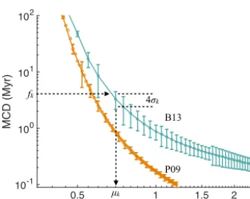
3
0.5 1 1.5 2
MCD (Myr)
10-1 100 101 102
B13
P09
fk
µk
4σk
Figure 6.MCD as a function ofθ for the B13 model (turquoise) and the P09 model (orange). Shown are the average MCD (solid lines) and 2-standard-deviation error bars computed from 100 sim-ulations. This graph is used to define the standard deviation of the feature noiseηkas well as the mean of the proposal distributionqk.
For the P09 model, we plot the standard deviations only for every otherθvalue for readability.
(shorter) than what we can actually compute with our model and bounded model parameters.
For each value ofθ on our grid, we perform 100 simula-tions and for each run compute average MCD. The mean and standard deviation of average MCD, computed from these simulations, are shown in Fig. 6. We occasionally observe large standard deviations for smallθk because only a few
re-versals may occur during these runs, which makes estimates of the standard deviations unreliable (see above). In this case, we assign a maximum standard deviation of 2.5 Myr.
We base our feature-error modelηkon this graph and pick ηk to be a zero-mean Gaussian with a standard deviationσk
that we read from the graph as illustrated by Fig. 6, i.e., for a givenfk, we use the standard deviation we computed for the
nearest point on our MCD–θgrid.
A feature fk defines ηk and then Eq. (11) defines a
feature-based likelihood. We define a prior distribution by the Gaussian p0,k(θk)=N(θk−1, σ02), where σ0=0.1 and
whereθk−1is the mean value we computed at the previous
time, k−1 (we describe what we did for the first time step
k=1 below). This results in the feature-based posterior
pk(θk|fk)∝exp −
1 2σk2(fk
−MF(θk))2−
1 2σ02 θk−1
−θk
2 !
.
We draw 100 samples from this posterior distribution by direct sampling with a proposal distribution qk(θk)=
N(µk, σq), whereσq=0.05 and whereµk is based on the
MCD–θgraph shown in Fig. 6, i.e., we chooseµkto be the θvalue corresponding to the MCD valuefkwe observe. We
have experimented with other values ofσq=0.05 and found
that howσq is chosen is not critical for obtaining the results
we present. We repeat this process for all but the very first
-100 -50 0
Time (Myr) 0.5
1 1.5 2 2.5
k
-100 -50 0
Time (Myr) 0.4
0.6 0.8 1
k
-100 -50 0
Time (Myr) 0
2 4 6 8 10
Mean chron duration (Myr) -100 -50 0
Time (Myr) 0
2 4 6 8 10
Mean chron duraiton (Myr)
B13 P09
(a) (b)
(c) (d)
Figure 7. (a)θkas a function of time for modified B13; 100 samples
of feature-based posterior distributionspk(θk|fk)(light turquoise)
and their mean (blue).(b) θk as a function of time for modified
P09; 100 samples of feature-based posterior distributionspk(θk|fk)
(light orange) and their mean (red).(c)Featuresfk computed by
drawing 100 samples (light turquoise) from the feature-based pos-terior distribution of the modified B13 model and their mean (blue).
(d)Featuresfk computed by drawing 100 samples (light orange) from the feature-based posterior distribution of the modified P09 model and their mean (red). The MCD feature extracted from the geomagnetic polarity timescale is shown in black.
of the featuresfk. For the first step,k=1, we set the prior
distribution equal to the proposal distribution.
Our results are illustrated in Fig. 7. Figure 7a and b show 100 samples of the posterior distributions pk(θk|fk) as a
function of time, as well as their mean. The panel on the right shows results for the modified B13 model, the panel on the left shows results for the modified P09 model. We note that, for both models,θkvaries significantly over time. The effect
that a time-varyingθhas on the MCD of the modified B13 and P09 models is illustrated in Fig. 7c and d, where we plot 100 features generated by the modified P09 and B13 models using the 100 posterior values ofθk shown in the top row.
We note a good agreement with the recorded feature (shown in black). This is perhaps not surprising, since we use the feature data to estimate parameters, which in turn reproduce the feature data. However, this is a basic check that our data assimilation framework produces meaningful results.
We further illustrate the results of the feature-based data assimilation in Fig. 8, where we plot the geomagnetic po-larity timescale as well as the dipole of the modified B13 and P09 models, generated by using a sequenceθk, drawn
-140 -120 -100 -80 -60 -40 -20 0 -1
0 1
-140 -120 -100 -80 -60 -40 -20 0
-1 0 1
Time (Myr)
-140 -120 -100 -80 -60 -40 -20 0
-1 0 1
Geomagnetic polarity timescale
Modified B13
Modified P09
P
ol
ari
ty a
nd
si
gne
d di
pol
e i
nt
ens
it
y
P
ol
ari
ty
(a)
(b)
(c)
Figure 8. (a)Geomagnetic polarity timescale.(b)Modified B13 model output withθkdrawn from the feature-based posterior distributions. (c)Modified P09 model output withθkdrawn from the feature-based posterior distributions.
The advantage of the feature-based approach in this prob-lem is that it allows us to calibrate the modified B13 and P09 models to yield a time-varying MCD in good agreement with the data (geomagnetic polarity timescale), where “good agreement” is to be interpreted in the feature-based sense. Our approach may be particularly useful for studying how flow structure at the core affects the occurrence of super-chrons. A thorough investigation of what our results imply about the physics of geomagnetic dipole reversals will be the subject of future work. In particular, we note that other choices for the standard deviationσ0, that defines expected
errors in the feature, are possible and that other choices will lead to different results. If one wishes to use the feature-based approach presented here to study the Earth’s deep inte-rior, one must carefully chooseσ0. Here we are content with
showing how to use feature-based data assimilation in the context of geomagnetic dipole modeling.
4.4 Example 4: parameter estimation for a Kuramoto–Sivashinsky equation
We consider the Kuramoto–Sivashinsky equation
∂φ
∂t = −θ∇
2φ− ∇4φ+ |∇φ|2,
where t∈ [0, T], the spatial domain is a two-dimensional square[x, y] ∈ [0,10π] × [0,10π]and the boundary condi-tions are periodic. Here ∇ =(∂/∂x, ∂/∂y)andθ is the pa-rameter we want to estimate. We use a uniform prior dis-tribution over[0,5]. As in earlier examples, our focus is on formulating likelihoods and our choice of prior is not critical to the points we wish to make when illustrating the feature-based techniques. The initial condition of the KS equation is a Gaussian random variable, which we choose as follows. We simulate the KS equation forT “time” units starting from uniformly distributed Fourier coefficients within the unit
hy-percube (see a few sentences below for how these simulations are done). We pickT large enough so thatφ (x, y, T )varies smoothly in space. We repeat this process 100 times to obtain 100 samples of solutions of the KS equation. The resulting sample mean and sample covariance matrix of the solution at timeT define the mean and covariance of the Gaussian which we use as a random initial condition below.
For computations we discretize the KS equation by the spectral method and exponential time differencing withδt= 0.005/θ. For a givenθ, we then computeφin physical space by Fourier transform and interpolation onto a 256×256 grid. The solution of the KS equation depends on the parameterθ
in a way that a typical spatial scale of the solution, i.e., the scale of the “valleys and hills” we observe, increases asθ de-creases, as illustrated by Fig. 9, where we show snapshots of the solution of the KS equation after 2500 time steps for two different choices of the parameterθ.
The data are 100 snapshots of the solution of the KS equa-tion obtained as follows. For a given θ, we draw an ini-tial condition from the Gaussian distribution (see above) and simulate for 2500 time steps. We save the solution on the 256×256 grid every 50 time steps. We repeat this process, with another random initial condition drawn from the same Gaussian distribution, to obtain another 50 snapshots of the solution. The 100 snapshots constitute a data set with a total number of more than 6 million points.
x x
x x
y
y
y
y
(a) (b)
(c) (d)
x x
x x
y
y
y
y
(e) (f)
(g) (h)
Figure 9. (a–d)Four snapshots of the solution of the KS equation withθ=1.55.(e–g)Four snapshots of the solution of the KS equation withθ=3.07.
We choose this feature because the parameter θ defines the spatial scale of the solution (see above) and this scale is connected to the length scale of a covariance function of a Gaussian process approximation of the solution. The length scale of the Gaussian process in turn defines the exponential decay of the eigenvalues of its associated covariance matrix and this decay is what we capture by our feature. In simple terms, the larger the length scale, the faster the decay of the eigenvalues.
It is important to note that the feature we construct does not depend on the initial conditions. This is the main advan-tage of the feature-based approach. Using the feature, rather than the trajectories, enables estimation of the parameter θ
without estimation of initial conditions. With a likelihood based on the mismatch of model and data, one has to estimate the parameterθandthe initial conditions, which makes the effective dimension of the problem large, so that the required computations are substantial. Most importantly, estimating the initial condition based on a mismatch of model output and data is difficult because the KS equation is chaotic. For these reasons, the feature-based approach makes estimation of the parameterθfeasible. Note that the feature has also reduced the effective dimension of the problem (see Sect. 3.3.4) be-cause the number of parameters to be estimated has been re-duced from the number of modes (2562) to 1. The price to be paid for this reduction in (effective) dimension is that the feature-based approach does not allow us to compute trajec-tories that match the data point-wise.
The feature-based likelihood is defined by the equation f =MF(θ )+η, η∼N(0,R), (12)
wheref =F(z)is the feature computed from the data,R is a 2×2 covariance matrix (see below) and whereMF is
Eigenvalue index
E
ige
nva
lue
20 40 60 80
10-4 10-2 100 102 104
Figure 10.Illustration of the computed feature. Eigenvalues of co-variance matrices of snapshots (dots) and log-linear fit (solid lines). Blue dots and red line correspond to a run withθ=1.55, turquoise dots and orange line correspond to a run withθ=3.07.
shorthand for the following computational steps for a given parameterθ:
i. Draw random initial conditions and obtain 100 snap-shots of the solution of the KS equation with parameter
θ.
ii. Interpolate snapshots onto 64×64 grid and compute sample covariance matrix.
iii. Compute largest eigenvalues of the sample covariance matrix and compute a log-linear fit.
The featureMF(θ )consists of the slope and offset of the
log-linear fit.