Numerical studies of non-local hyperbolic partial differential
equa-tions using collocation methods
Khalid Karam Ali∗
Mathematics Department, Faculty of Science, Al-Azhar University, Nasr City (11884), Cairo, Egypt.
E-mail: [email protected].
Kamal Raslan Raslan
Mathematics Department, Faculty of Science, Al-Azhar University, Nasr City (11884), Cairo, Egypt.
E-mail: kamal [email protected]
Adel Rashad Hadhoud
Mathematics Department, Faculty of Science, Menoufia University, Shebein El-Koom, Egypt. E-mail: [email protected]
Abstract The non-local hyperbolic partial differential equations have many applications in sciences and engineering. A collocation finite element approach based on exponential cubic B-spline and quintic B-spline are presented for the numerical solution of the wave equation subject to nonlocal boundary condition. Von Neumann stability analysis is used to analyze the proposed methods. The efficiency, accuracy and stability of the methods are assessed by applying it to the test problem. The results are found to be in good agreement with known solutions and with existing collocation schemes in literature.
Keywords. Collocation methods, Exponential cubic B-spline, Quintic B-spline, Finite difference, Wave
equation.
2010 Mathematics Subject Classification.
1. Introduction
Many physical phenomena are modeled by non-classical hyperbolic boundary value problems with nonlocal boundary conditions. In place of the classical specification of boundary data, we impose a nonlocal boundary condition. Partial differential equations with non-local boundary conditions have received much attention in the last twenty years.
In this paper we will consider a non-classic hyperbolic equation [3,24]. We consider the following problem of this family of equations:
utt−µ uxx=f(x, t), a≤x≤b, 0≤t≤T, (1.1)
Received: 9 January 2018 ; Accepted: 14 May 2018. ∗Corresponding author.
with the initial condition
u(x,0) =g(x), a≤x≤b, (1.2)
and the boundary conditions
u(a, t) =p1(t), 0≤t≤T, (1.3)
u(b, t) =p2(t), 0≤t≤T, (1.4)
ux(a, t) =h(t), 0≤t≤T, (1.5)
and the non-local boundary condition
Z b
a
u(x, t)dx=m(t), (1.6)
where the functionsf(x, t), g(x), p1(t), p2(t), h(t) and m(t) and the parameter µ are known. The exact solutions and numerical solutions of linear and nonlinear partial differential equations and nonlinear systems of partial differential equations are very important in applied science, for example, exact solutions of coupled GEWE and the space-time fractional RLW and MRLW equations they were obtained by Raslan et al. [20, 23], the KDV equation solved by Raslan et al.[18, 22], the Hirota-Satsuma coupled KDV equation studied by Raslan et al. [13]. Also, the Hirota equation has been solving by Raslan et al. [17,19]. The generalized long wave equation system has been solved by El- Danaf et al.[6, 7]. The coupled-BBM system has been solved by Raslan et al. [12]-[14]. Coupled Burgers’ equations has been studied by Ali et al.[9] and by Raslan et al. [15,16].
There are many studies of our equation such as, Ang solved the problem using a scheme based on an integro-differential equation and local interpolating functions [1]. Then, B-spline functions were found to be an efficient method for solving wave equation such as, Dehghan et al [4], Khury et al. [10], Goh et al. [8], Caglar et al. [2] and Zin et al.[11]. Also, M. Dehghan and A. Shokri used a meshless method [5].
In this paper, we apply the exponential cubic B-spline and Quintic B-spline meth-ods for computing an approximate solution to (1.1)-(1.6).
This paper is organized as follows. Section 2 is description of the collocation methods for solving equations (1.1)-(1.6). In section 3, some numerical results are presented to demonstrate the efficiency of the methods. Some concluding remarks are presented in section 4.
2. Description of collocation B-spline methods
In this section, we discuss collocation B-spline methods for solving numerically the one-dimensional hyperbolic equation (1.1). To construct numerical solution, consider nodal points (xj, tn) defined in the region [a, b]×[0, T] where
a=x0< x1< ... < xN =b, h=xj+1−xj= b−a
2.1. Description of exponential cubic B-spline method.
Our approach for one-dimensional hyperbolic equation using collocation method with exponential cubic B-spline is to seek an approximate solution as
UN(x, t) = N+1
X
j=−1
cj(t)Bj(x), (2.1)
wherecj(t) are to be determined for the approximated solutionsUN(x, t),to the exact solutionsu(x, t) at the point (xj, tn) whilstBj(x) are exponential cubic B-spline basis functions defined by
Bj(x) = b2
(xj−2−x) −
1
p(sinh (p(xj−2−x)))
, xj−2≤x≤xj−1,
a1 + b1(xj−x) +c1 exp (p(xj−x))
+d1exp (−p(xj−x)) xj−1≤x≤xj,
a1 + b1(x−xj) +c1 exp (p(x−xj))
+d1exp (−p(x−xj)), xj≤x≤xj+1,
b2
(x−xj+2) −
1
p(sinh (p(x−xj+2)))
, xj+1≤x≤xj+2,
0 otherwise ,
(2.2) where
a1 =
p h c
p h c−s, b1 = p 2
c(c−1) +s2 (p h c−s) (1−c)
,
b2 =
p
2 (p h c−s), c1 = 1 4
exp (−p h) (1−c) +s(exp (−p h)−1) (p h c−s) (1−c)
,
d1 = 1 4
exp (p h) (1−c) +s(exp (p h)−1) (p h c−s) (1−c)
,
s= sinh (p h), c=coh (p h), h=b−a N .
Using approximate function (2.1) and exponential cubic B-spline functions (2.2), the approximate valuesU(x) and their derivatives up to second order are determined in terms of the time parameterscj(t) as
Uj=U(xj) =m1cj−1+cj+m1cj+1,
Uj0 =U0(xj) =m2cj−1−m2cj+1,
U00
j =U00(xj) =m3cj−1−2m3cj+m3cj+1,
(2.3)
wherem1=
(s−p h)
2 (p h c−s), m2=
p(1−c)
2 (p h c−s), m3=
p2s 2 (p h c−s). To apply the proposed method, we can rewrite (1.1) as
∂2u(x, t)
∂t2 −µ
∂2u(x, t)
∂x2 −f(x, t) = 0,
get
Ujn+1−2Un j +U
n−1
j
k2 −µ
"
Uxxnj+1+Uxxnj 2
#
−f(xj, tn) = 0, (2.4)
wherek= ∆t is the time step.
On substituting the approximate solution forU and its derivatives from Eq. (2.3) at the knots in Eq. (2.4) yields the following difference equation with the variables cj(t).
A1cnj−+11 +A2cjn+1+A1cnj+1+1=
A3cnj−1+A4cnj +A3cnj+1−m1cnj−−11−c
n−1
j −m1cjn+1−1+k2f(xj, tn), (2.5)
whereA1=m1−
k2µ
2 m3, A2= 1 +k 2µ m
3, A3= 2m1+
k2µ 2 m3, A4= 2−k2µ m3.
It is clear that the system (2.5) consists of (N+ 1) linear equations in the (N+ 3) unknown (cn
−1, cn0, ..., cnN, cnN+1)T. Hence, the following two additional equation from the boundary conditions given in (1.3) and (1.6) are needed for calculation.
(1)
m1cn−1+c
n
0+m1cn1 =p1(tn), (2.6)
(2)
m2cnN−1−m2cnN+1−m2cn−1+m2cn1 =m00(tn)−
Z b
a
f(x, tn)dx. (2.7)
Then the system is tridiagonal matrix system of dimension (N+ 3)×(N+ 3) that can be solved by any algorithm.
The above system requires two initial time levels att= 0,andt= ∆t=k,we can evaluate the initial conditions att= 0 and t=kas
At level timen= 0 (t= 0)
UN(xj,0) = N+1
X
j=−1
c0jBj(x) =m1c0j−1+c 0
j+m1c0j+1=g(x), j= 0,1, ..., N.
(2.8)
At level timen= 1 (t=k)
UN(xj, k) = N+1
X
j=−1
c1jBj(x) =m1c1j−1+c 1
j+m1c1j+1=g(x), j= 0,1, ..., N.
(2.9)
It is clear that the systems (2.8) and (2.9) consists of (N+ 1) linear equations in the (N+ 3) unknowns (c0−1, c00, ..., c0N, c
0
N+1)
T,(c1
−1, c10, ..., c1N, c
1
N+1)
T.
Table 1. Numerical errors at the grid points for various mesh sizes withk= 0.01 att= 5.
x
h= 0.1, p=
3.456×10⁻⁵
Exponential cubic B-spline
h= 0.02 p=
3.456×10⁻⁵ Exponential cubic B-spline
h= 0.01 p=
3.456×10⁻⁵ Exponential cubic B-spline
h= 0.02 Quintic B-spline
h= 0.01 Quintic B-spline 0.1 0.2 0.3 0.4 0.5 0.6 0.7 0.8 0.9 1.97090 E-3 2.88999 E-3 2.71061 E-3 1.61636 E-3 3.1214 E-16 1.61636 E-3 2.71061 E-3 2.88999 E-3 1.97090 E-3 3.83207 E-5 5.97271 E-5 5.83163 E-5 3.55555 E-5 5.71213E-16 3.55555 E-5 5.83163 E-5 5.97271 E-5 3.83207 E-5 2.14171 E-5 2.86301 E-5 2.53084 E-5 1.45997 E-5 4.16733E-16 1.45997 E-5 2.53084 E-5 2.86301 E-5 2.14171 E-5 1.64398 E-4 2.71918 E-4 2.70807 E-4 1.65951 E-4 1.99285E-16 1.65951 E-4 2.70807 E-4 2.71918 E-4 1.64398 E-4 5.73333 E-5 9.57796 E-5 9.63597 E-5 5.93989 E-5 3.54061E-15 5.93989 E-5 9.63597 E-5 9.57796 E-5 5.73333 E-5
Table 2. Compare absolute errors of our schemes with absolute er-rors of [8] and [11] at k= 0.01 andt= 5.
x h= 0.01
p =
3.456×10⁻⁵ Exponential cubic B-spline
h= 0.01 Quintic B-spline
h= 0.01[8] cubic B-spline
h= 0.01[11]
0.1 0.2 0.3 0.4 0.5 0.6 0.7 0.8 0.9 2.14171 E-5 2.86301 E-5 2.53084 E-5 1.45997 E-5 4.16733E-16 1.45997 E-5 2.53084 E-5 2.86301 E-5 2.14171 E-5 5.73333 E-5 9.57796 E-5 9.63597 E-5 5.93989 E-5 3.54061E-15 5.93989 E-5 9.63597 E-5 9.57796 E-5 5.73333 E-5 7.97 E-5 1.21 E-4 1.15 E-4 6.88 E-5 2.03E-13 6.88 E-5 1.15 E-4 1.21 E-4 7.97 E-5 7.39 E-5 1.12 E-4 1.07 E-4 6.40 E-5 5.05E-15 6.40 E-5 1.07 E-4 1.12 E-4 7.39 E-5
2.1.1. Stability analysis of the method.
Our stability analysis will be based on the Von-Neumann concept in which the growth factor of a typical Fourier mode defined as
cnj =ζnexp(ijφ), (2.10)
g= ζ n+1
where,φ=k h,k is the mode number,i=√−1 andg is the amplification factor of the schemes. We will apply the stability of the exponential cubic scheme (2.5).Thus, f(x, t) in (1.1) is assumed to be 0.
Substituting (2.10) into the difference (2.5), we get
(2A1cos (φ) +A2) g2−(2A3cos (φ) +A4)g+ (2m1cos (φ) + 1) = 0, (2.11) Let
A= (2A1cos (φ) +A2), B = (2A3cos (φ) +A4), C = (2m1cos (φ) + 1), Then, Eq. (2.11) becomes
A g2−B g+C= 0, (2.12)
Applying the Routh–Hurwitz criterion on Eq. (2.12), the necessary and sufficient condition for Eq. (2.5) to be stable as follows:
Using the transformation g = 1 +ν
1−ν and simplifying, Eq. (2.12) takes the form [25]
(A+B+C)ν2+ 2 (A−C) ν+ (A−B+C) = 0. The necessary and sufficient condition for|g| ≤1 is that
(A+B+C)≥0, (A−C)≥0, (A−B+C)≥0. It can be easily proved that
(A+B+C) = 8m1 cos (φ) + 4≥0, (A−C) =k2µ m
3(1−cos (φ))≥0, (A−B+C) = 2k2µ m
3(1−cos (φ))≥0.
It is evident that the scheme is unconditionally stable. It means that there is no restriction on the grid size, i.e. onhand, buthshould be chosen in such a way that the accuracy of the scheme is not degraded
2.2. Description of quintic B-spline method.
The quintic B-spline basis functions at knots are given by: Bj(x) =
1 h5
(x−xj−3)5, xj−3≤x≤xj−2
(x−xj−3)5 −6 (x−xj−2)5, xj−2≤x≤xj−1
(x−xj−3)5 −6 (x−xj−2)5 + 15(x−xj−1)5, xj−1≤x≤xj
(−x+xj+3)5 + 6 (x−xj+2)5 −15(x−xj+1)5, xj≤x≤xj+1
(−x+xj+3)5 + 6 (x−xj+2)5, xj+1≤x≤xj+2
(−x+xj+3)5, xj+2≤x≤xj+3
0 otherwise
(2.13) ExpressingU(x, t) by using quintic B-spline functionsBj(x) and the time dependent parameterscj(t) forU(x, t), the approximate solution can be written as:
UN(x, t) = N+2
X
j=−2
Using approximate function (2.14) and quintic B-spline functions (2.13), the approx-imate valuesU(x) and their derivatives up to second order are determined in terms of the time parameterscj(t), as
Uj=U(xj) =cj−2+ 26cj−1+ 66cj+ 26cj+1+cj+2,
Uj0 =U0(xj) = 5
h(cj+2+ 10cj+1−10cj−1−cj−2), Uj00=U00(xj) =
20
h2(cj−2+ 2cj−1−6cj+ 2cj+1+cj+2).
(2.15)
On substituting the approximate solution forU and its derivatives from Eq. (2.15) at the knots in Eq. (2.4) yields the following difference equation with the variablescj(t).
B1cnj−+12 +B2cjn−+11 +B3cnj+1+B2cjn+1+1+B1cnj+2+1=B4cnj−2+B5cnj−1 +B6cnj +B5cjn+1+B4cnj+2−c
n−1
j−2 −26c
n−1
j−1 −66c
n−1
j −26c n−1
j+1 −cnj+2−1+k2f(x
j, tn),
(2.16)
where
B1= 1− 20k2µ
2h2 , B2= 26− 20k2µ
h2 , B3= 66 +
120k2µ 2h2 ,
B4= 2 + 20k2µ
2h2 , B5= 52 + 20k2µ
h2 , B6= 132−
120k2µ 2h2 .
It is clear that the system (2.16) consists of (N+ 1) linear equations in the(N + 5) unknown (cn
−2, cn−1, cn0, ..., cNn, cnN+1, cnN+2)T. Hence, the following four additional equation from the boundary conditions given in (1.3), (1.4), (1.5) and (1.6) are needed for calculation.
(1)
cn−2+ 26cn−1+ 66cn0+ 26cn1 +cn2 =p1(tn), (2.17)
(2)
cnN−2+ 26cnN−1+ 66cnN+ 26cnN+1+cnN+2=p2(tn), (2.18)
(3) 5 h(c
n
2 + 10c
n
1−10c
n −1−c
n
−2) =h(tn), (2.19)
(4) 5 h(c
n
N+2+ 10c
n
N+1−10c
n N−1−c
n N−2)−
5 h(c
n
2 + 10c
n
1 −10c
n −1−c
n −2) =m00(tn)−Rb
af(x, tn)dx.
(2.20)
Then the system is penta-diagonal matrix system of dimension (N+ 5)×(N+ 5) that can be solved by any algorithm.
At level timen= 0 (t= 0)
UN(xj,0) = N+2
X
j=−2
c0jBj(x)
=c0j−2+ 26c 0
j−1+ 66c 0
j+ 26c
0
j+1+c 0
j+2=g(x),
j= 0,1, ..., N.
(2.21)
At level timen= 1 (t=k)
UN(xj, k) = N+2
X
j=−2
c1j Bj(x)
= 5 h −c
1
j−2−10c 1
j−1+ 10c 1
j+1+c 1
j+2
=g(x),
j= 0,1, ..., N.
(2.22)
It is clear that the systems (2.21) and (2.22) consists of (N+ 1) linear equations in the (N+ 5) unknown (c0
−2, c0−1, ..., c0N+1, c 0
N+2)
T, (c1
−2, c1−1, ...., c1N+1, c 1
N+2)
T.Hence, to solve these systems we can be using (2.17), (2.18), (2.19) and (2.20) at two time levels at n = 0, and n = k. Then the system is penta-diagonal matrix system of dimension (N+ 5)×(N+ 5) that can be solved by any algorithm.
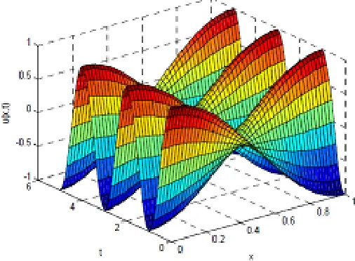
Figure 2. Space-time graph of numerical solution of our problem using quintic B-spline with h= 0.01 andk= 0.01.
2.2.1. Stability analysis of the method.
Our stability analysis will be based on the Von-Neumann concept in which the growth factor of a typical Fourier mode defined as
cnj =ζnexp(ijφ), (2.23)
g= ζ n+1
ζn ,
where, φ=k h , k is the mode number, i=√−1 and g is the amplification factor of the schemes. We will apply the stability of the quintic scheme (2.16).
Substituting (2.23) into the difference (2.16), we get
(2B1cos (2φ) + 2B2cos (φ) +B3)g2−(2B4cos (2φ) + 2B5cos (φ) +B6)g+ (2 cos (2φ) + 52 cos (φ) + 66) = 0.
(2.24)
Let
D= (2B1cos (2φ) + 2B2cos (φ) +B3) ,
E= (2B4cos (2φ) + 2B5cos (φ) +B6),
F = (2 cos (2φ) + 52 cos (φ) + 66).
Then, Eq. (2.24) becomes
Dg2−E g+F = 0. (2.25)
Applying the Routh–Hurwitz criterion on Eq. (2.25), the necessary and sufficient condition for Eq. (2.16) to be stable as follows:
Using the transformation g = 1 +ν
1−ν and simplifying, Eq. (2.25) takes the form [25]
(D +E+F)ν2+ 2 (D−F) ν+ (D −E+F) = 0. The necessary and sufficient condition for|g| ≤1 is that
(D+E+F)≥0, (D−F)≥0, (D −E+F)≥0.
It can be easily proved that
(D+E+F) = 8 cos (2φ) + 208 cos (φ) + 264≥0,
(D−F) = 20k 2µ
2h2 (6−2 cos (2φ)−4 cos (φ))≥0, (D−E+F) =40k
2µ
2h2 (6−2 cos (2φ)−4 cos (φ))≥0.
It is clear that the scheme is unconditionally stable. It means that there is no restric-tion on the grid size, i.e. on hand, but hshould be chosen in such a way that the accuracy of the scheme is not degraded
3. Numerical Tests and Results of wave equation
In this section, we present numerical example to test validity of our schemes for solving wave equation.
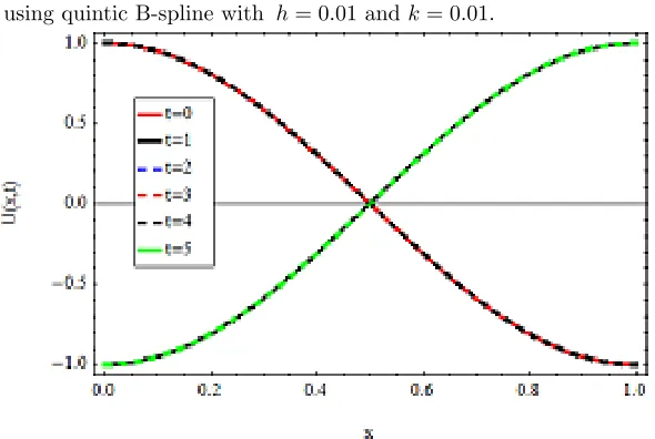
We consider the wave equation is considered as [8]-[11]
utt−µ uxx= 0, 0≤x≤1, 0≤t≤T, with the initial condition
u(x,0) = cos(π x), 0≤x≤1,
and the boundary conditions
u(0, t) = cos(π x), 0≤t≤T,
u(1, t) = 0.5{cos [π( 1 +t)] + cos [π( 1−t)]}, 0≤t≤T, ux(0, t) = 0, 0≤t≤T,
and the non-local boundary condition Z 1
0
u(x, t)dx= 0.
The analytical solution is given by
u(x, t) = 0.5{cos [π(x+t)] + cos [π(x−t)]},0≤x≤1, 0≤t≤T.
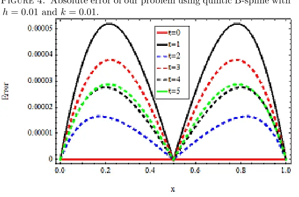
Table 2 shows that the present methods gives smaller absolute error compare with [8] and [11].
4. Conclusion
In this work, a numerical methods incorporating finite difference approach with exponential cubic B-spline and quantic B-spline had been developed to solve one-dimensional wave equation. B-spline functions had been used to interpolate the solu-tion inx-direction and finite difference approach had been applied to discretize the time derivative. Based on von Neumann stability analysis, this approach was proved to be unconditionally stable.
The problem was tested. It was found that the solutions are approximated very well. Tables 1 and 2 showe the errors obtained from present methods are less than the errors obtained from the methods proposed in literature. Hence, we conclude that this present methods approximate the solutions very well. Hence, we conclude that the quintic B-spline method approximates the solutions very well.
References
[1] W. T. Ang, A numerical method for the wave equation subject to a non-local conservation condition, Applied Numerical Mathematics,56(2006), 1054–1060.
[2] H. Caglar, N. Caglar, and K. Elfauturi,B-spline interpolation compared with finite difference, finite element and finite volume methods which applied to two-point boundary value problems, Applied Mathematics and Computation,175(1) (2006), 72–79.
[3] M. Dehghan,On the solution of an initial-boundary value problem that combines Neumann and integral condition for the wave equation, Numerical Methods for Partial Differential Equations, 21(1) (2005), 24–40.
[4] M. Dehghan and M. Lakestani,The use of cubic B-spline scaling functions for solving the one-dimensional hyperbolic equation with a nonlocal conservation condition, Numerical Methods for Partial Differential Equation,23(2007), 1277–1289.
[5] M. Dehghan and A. Shokri,A meshless method for numerical solution of the one-dimensional wave equation with an integral condition using radial basis functions, Numerical Algorithms, 52(3)(2009), 461–477.
[6] T. S. EL-Danaf, K. R. Raslan, and K. K. Ali, Collocation method with cubic B- Splines for solving the generalized long wave equation, Int. J. of Num. Meth. and Appl., 15(1) (2016), 39–59.
[7] T. S. EL-Danaf, K. R. Raslan and K. A. Khalid,New numerical treatment for the generalized regularized long wave equation based on finite difference scheme, Int. J. of S. Comp. and Eng. (IJSCE),4(2014), 16–24.
[8] J. Goh, A. Abd. Majid, and A. I. Md Ismail,Numerical method using cubic B-spline for the heat and wave equation, Computer and Mathematics with Application,62(12) (2011), 4492–4498. [9] K. A. Khalid, K. R. Raslan, and T. S. El-Danaf, Non-polynomial spline method for solving
coupled Burgers’ equations, Computational Methods for Differential Equations, 3(3) (2016), 218–230.
[10] S. A. Khuri and A. Sayfy,A spline collocation approach for a generalized wave equation subject to non-local conservation condition, Applied Mathematics and Computation, 217(8) (2010), 3993–4001.
[12] K. R. Raslan, T. S. El-Danaf, and K. A. Khalid, An efficient approach to numerical study of the coupled-bbm system with b-spline collocation method, Communication in Mathematical Modeling and Applications,1(3) (2016), 5–15.
[13] K. R. Raslan, T. S. El-Danaf, and K. A. Khalid,Application of linear combination between cubic B-spline collocation methods with different basis for solving the KdV equation, Computational Methods for Differential Equations,4(3) (2016), 191–204.
[14] K. R. Raslan, T. S. El-Danaf, and K. A. Khalid, Application of septic B-spline collocation method for solving the coupled-BBM system, Appli. and Comput. Math.,5(5) (2016), 2–7. [15] K. R. Raslan, T. S. El-Danaf, and K. A. Khalid,Collocation method with cubic
trigonomet-ric B-splines algorithm for solving Coupled Burgers’ Equations, Far East Journal of Applied Mathematics,95(2) (2016), 109–123.
[16] K. R. Raslan, T. S. El-Danaf, and K. A. Khalid,Collocation method with quintic B-splines method for solving coupled Burgers’ equations, Far East Journal of Applied Mathematics,96(1) (2017), 55–75.
[17] K. R. Raslan, T. S. El-Danaf, and K. A. Khalid, Collocation method with quintic B-spline method for solving the Hirota equation, Journal of Abstract and Computational Mathematics, 1(2016), 1–12.
[18] K. R. Raslan, T. S. El-Danaf, and K. A. Khalid,Collocation method with quantic B-spline method for solving hirota-satsuma coupled KDV equation, International Journal of Applied Mathematical Research,5(2) (2016), 123–131.
[19] K. R. Raslan, T. S. El-Danaf, and K. A. Khalid,Finite difference method with different high order approximations for solving complex equation, New Trends in Mathematical Sciences,5(1) (2017), 114–127.
[20] K. R. Raslan, T. S. El-Danaf, and K. A. Khalid,New exact solution of coupled general equal width wave equation using sine-cosine function method, Journal of the Egyptian Mathematical Society,25(2017), 350–354.
[21] K. R. Raslan, T. S. El-Danaf, and K. A. Khalid,Numerical treatment for the coupled-BBM system, Journal of Modern Methods in Numerical Mathematics,7(2)(2016), 67–79.
[22] K. R. Raslan, T. S. El-Danaf, and K. A. Khalid,New numerical treatment for solving the KDV equation, Journal of Abstract and Computational Mathematics,2(1) (2017), 1–12.
[23] K. R. Raslan, K. A. Khalid, and M. A. Shallal ,Solving the space-time fractional RLW and MRLW equations using modified extended Tanh method with the Riccati equation, British Jour-nal of Mathematics and Computer Science,21(4) (2017), 1–15.
[24] F. Shakeri and M. Dehghan, The method of lines for solution of the one-dimensional wave equation subject to an integral conservation condition, Computer and Mathematics with Appli-cations,56(9) (2008), 2175–2188.
![Table 2. Compare absolute errors of our schemes with absolute er-rors of [8] and [11] at k = 0.01 and t = 5.](https://thumb-us.123doks.com/thumbv2/123dok_us/8943504.1852872/5.612.129.482.141.320/table-compare-absolute-errors-schemes-absolute-er-rors.webp)