FPGA Implementation of NLMS Algorithm for Identification of unknown system.

FPGA Implementation of NLMS Algorithm

for Identification of unknown system.

K. R. Rekha *,

E&C Dept, M. G. R. University, Chennai, India Dr B. S. Nagabushan **

** Sanlab Technologies, Bangalore, 560038, India And Dr K.R..Nataraj ***

*** SJB Institute of Technology, Bangalore, 560060, India

Abstract

This paper proposes a VHDL implementation of a variable step size Least Mean Square (NLMS) adaptive algorithm. The envisaged application is the identification of an unknown system. The good convergence of NLMS algorithm has made us to choose it. It also has good stability. Adaptive filtering constitutes one of the core technologies in digital signal processing and finds numerous application areas in science as well as in industry. Adaptive filtering techniques are used in a wide range of applications, including system identification, adaptive equalization, adaptive noise cancellation, wire less communication and echo cancellation. A HDL implementation is developed for a 4th order NLMS adaptive filter. As compared conventional LMS it has been proven that NLMS Algorithm has good behavior. ModelSim simulations results altogether with plots obtained in Matlab prove the same.

Keywords : Adaptive filters , Digital signal processing, NLMS, LMS. Introduction

1. Need for NLMS

One of the most popular adaptive algorithms available in the literature is the stochastic gradient algorithm also called least-mean-square (LMS) [1], [2]. It has been popularized due to its simplicity in implementation. It is the main reason for its usage in wide application. Many communication systems have Least – Mean - Square (LMS) adaptive filter as their main component; traditionally, such adaptive filters are implemented in Digital Signal Processors (DSPs). If performance is the key requirement, then they are implemented in ASICs. However, many high-performance DSP systems, including LMS adaptive filters, may be implemented using Field Programmable Gate Arrays (FPGAs) due to some of their attractive advantages. Such advantages include flexibility and programmability, but most of all, availability of tens to hundreds of hardware multipliers available on a chip [3].

The other advantages of NLMS adaptive filter are robust behaviour when implemented in finite-precision hardware, well understood convergence behaviour and computational simplicity for most situations, which make it as different from other adaptive algorithms.

The simple well behaved NLMS adaptive filter algorithm is commonly used in applications where a system has to adapt to its environment. Architectures are examined in terms of the following criteria: speed, power consumption and FPGA resource usage [6].Modern FPGAs contain many resources that support DSP applications .These resources are implemented in the FPGA fabric and optimized for high performance and low power consumption [7].

2. Normalised Least Mean Square Algorithm

2.1 Introduction to Adaptive Filters

Vol. 2(11), 2010, 6391-6407 information about a quantity of interest at time‘t’ by using data measured up to and including time t. If the inputs to the filter are stationary, the resulting solution of the filtering problem is known as the Wiener Filter, which is said to be optimum in mean square sense. But it requires a priori information about the statistics of the data to be processed. If the environment is unknown then another efficient method is to use an adaptive filter using recursive algorithm. The algorithm starts with some predetermined set of initial conditions, representing whatever we know about the environment. In stationary environment it is expected that the adaptive filter converge to the optimum Wiener solution after successive iterations of the algorithm. In non- stationary environment, the algorithm can track time variations in the statistics of input data, provided that the variations are sufficiently slow.

One of the core technologies in digital signal processing is Adaptive filtering. We find numerous application areas in science as well as in industry. Adaptive filtering techniques are used in a wide range of applications, including system identification, adaptive equalization, adaptive noise cancellation, and echo cancellation. Characteristics of signals that are generated by systems of the above application are not known a priori. Under this condition, a significant improvement in performance can be achieved by using adaptive rather than fixed filters. An adaptive filter is a self-designing filter that uses a recursive algorithm (known as adaptation algorithm or adaptive filtering algorithm) to “design itself.” The algorithm starts from an initial guess; chosen based on the a priori knowledge available to the system, then refines the guess in successive iterations, and converges, eventually, to the optimal Wiener solution in some statistical sense [9]. Adaptive filters are used in applications to estimate response of unknown system. Every ones desire is to perform this estimation as accurately and quickly as possible.

The one basic common feature of adaptive filters is: An input vector and a desired response are used to compute an estimation error, which in turn is used to control the values of a set of adjustable filter coefficients by a feedback loop and an algorithm.

Adaptive filters can be implemented either in Finite Impulse Response (FIR) form or in Infinite Impulse Response (IIR) form. FIR filters are usually implemented in non-recursive structures, whereas IIR filters employ recursive realizations. In the case of FIR realizations, the most widely used adaptive filter structure is the transversal filter, also known as tapped delay line structure

An adaptive filter is time-varying since their parameters are continually changing in order to meet certain performance requirement. Usually the definition of the performance criterion requires the existence of a reference signal, which is absent in time-invariant filters. The general set up of an adaptive filtering environment is illustrated in Figure 3-1, where n is the iteration index, x(n) denotes the input signal, y(n) is the adaptive filter’s output signal, and d(n) defines the reference or desired signal. The error signal e(n) is the difference between the desired d(n) and filter output y(n). The error signal is used as a feedback to the adaptation algorithm in order to determine the appropriate updating of the filter’s coefficients, or tap weights. The minimization objective is for the adaptive filter’s output signal matching the desired signal in some sense.

The minimization objective can be viewed as a function of the input, desired, and output signals, or consequently a function of the error signal. One of the most commonly used objectives is to minimize the mean square error, that is, the objective function is defined as

d(k)

+

x(k)

y(k)

-

e(k)

Fig.2.1: General set up of an adaptive filtering environment

2.2 Least mean square algorithm

Before deriving the NLMS adaptive algorithm we should start from wiener filters and by using iterative search method we derive the LMS by which we derive the equations for NLMS

2.2.1Mean Square Error criterion

Figure 2.2 illustrates a linear filter [9] which estimates the desired signal d(n)from input x(n).Assume that d(n) and x(n) are samples of infinite length, random process.

Fig.2.2: A Liner Adaptive filter used for Estimating Desired Signal d(n)

The filter output is y(n) and the estimation error is given by e(n). The performance of the filter is determined by the size of the estimation error, that is, a smaller estimation error indicates a better filter performance. As the estimation error approaches zero, the filter output y(t) approaches the desired signal d(t).

Clearly, we require the estimation error to be as small as possible. In simple words, in our design of the filter parameters, we choose an appropriate function of this estimation error as a performance or cost function and select the set of filter parameters which optimizes the cost function.

In Wiener filters, the cost function is chosen to be

ξ = E[e(n)2_{] ……… (2.2)}

where E[.] denotes expectation or ensemble average since both d(n) and x(n) are random processes. ADAPTIVE

FILTER

ADAPTIVE ALGORITHM

Vol. 2(11), 2010, 6391-6407

Wiener Filter: Transversal, Real-Valued Case [1], [2]

Consider an adaptive transversal filter [8] as shown in Figure 2.2. Assume that the filter input x(n) and the desired output d(n) are real-valued stationary processes. The filter tap weights w0, w1 ,…….., wN-1 are also assumed to be real-valued, where N equals the number of delay units or tap weights.

We can define the filter input x(n) and tap-weight vectors, w, as column vectors,

x(n) = [x(n) x(n-1) .... x(n – N+1)] ……… 2-3

w = [w0 w1 …….wN-1] ……… 2-4

The filter output is defined as

y(n) =∑

w x n

i

Subsequently, the error signal can be written as

e(n) = d(n) - y(n) = d(n) - w' x (n) = d(n) - x '(n)w ………… 2-6 Substituting (2-6) into (2-2), we obtain the cost function,

ξ = E[e(n) 2_{] = E[(d(n) - w' x (n))(d(n) - x'(n) w)] ……… 2-7} Expanding the last expression of (2-7), we obtain

ξ =E[d2 _{(n)]-E[d(n) x'(n)w ]-E[d(n) w'x (n)] +E[w'x(n)x'(n)w] …… 2-8}

Fig.2.3: Structure of an Adaptive Transversal Filter

ξ =E[d2 _{(n)]-E[d(n) x'(n) ]w- w'E[d(n) x (n)] + w'E[x(n)x'(n)] w ….. 2-9} Next, we can express E[d(n) x(n)] as an N x 1 cross correlation vector

p = E[d(n)x(n)] = [p0 p1 ...pN-1]' ……… 2-10 and E[x(n)x'(n)] as a N x N auto correlation matrix

R = E[x(n)x’(n)]=

_,

,

,

,

,

,

….. 2-11

From (2-10), p'= E[d(n)x' (n)] and hence, p'w =w'p =>

E[d(n)x' (n)]w = E[d(n)x' (n)]w'. Subsequently, we get

ξ =E[d2_{(n)] -E[d(n) x'(n)]w-w' E[d(n) (n)]+w' E[x(n) x'(n)]w}

=E[d2_{(n)]-2p 'w+ w'Rw ...………… 2.12}

This is a quadratic function of tap-weight vector w with a single global minimum [9]. To obtain the set of filter tap weights that minimizes the cost function ξ, we need to solve the system of equations that results from setting the partial derivatives of ξ with respect to every tap weight of the filter (i.e. the gradient vector) to zero. That is

ξ

0

Note that the gradient vector in (2-13) can also be expressed as

ξ = 0 ……… 2.14

= ……… 2.15

and 0 on the right hand side of (2-14) denotes the column vector consisting of N zeros.

In [2], it is further proven that the partial derivatives of x with respect to the filter tap weights can be solved such that

ξ = 2Rw - 2p ……… 2.16

By letting ξ =0, we get the following equations, in which the optimum set of Wiener filter tap weights can be obtained,

Vol. 2(11), 2010, 6391-6407

 w =R-1p =w0 ……… 2.17

Where w0 indicates the optimum tap-weight vector. This equation is known as the Wiener-Hopf equation and

can be solved to obtain the tap-weight vector which corresponds to the minimum point of the cost function.

2.2.2 Iterative Search Algorithm

As we learned in the previous section, the Wiener-Hopf equation can be solved to obtain the optimum filter tap-weights by minimizing a cost function, if the required statistics of the underlying signals R and p are available.

Although this method is straightforward, it presents serious computational difficulties, especially when the filter contains a large number of tap weights and the input data rate is high [8].

An alternative [9] is to use an iterative search algorithm that starts at some arbitrary initial point in the tap-weight vector space and moves progressively towards the optimum filter tap-tap-weight vector in steps. Each step is chosen with the aim of reducing the cost function. This principle of finding the optimum filter tap-weight vector by progressive minimization of the underlying cost function by means of an iterative algorithm is central to the development of adaptive algorithms (e.g. LMS). In simplified terms, adaptive algorithms are actually iterative search algorithms derived for minimizing the cost function by replacing the true statistics with estimates obtained [9].

In the coming section, we will discuss an iterative search method known as Method of Steepest Descent. The LMS algorithm is implemented based on this method.

2.2.3 Method of Steepest Descent

Assume that the cost function to be minimized is convex, we may start with an arbitrary point on the performance surface and take a small step in the direction in which the cost function decreases fastest. This corresponds to a step along the steepest-descent slope of the performance surface at that point. Repeating this successively, convergence towards the bottom of the performance surface (corresponding to the set of parameters that minimize the cost function) is guaranteed [9].

The method of steepest descent is an alternate iterative search method to find w0 (in contrast to solving the

Wiener-Hopf equation directly), and uses the following procedures [8] to search for the minimum point of the cost function of a set of filter tap-weights,

1. Begin with an initial guess of the filter tap weights whose optimum values are to be found for minimizing the cost function. Unless some prior knowledge is available, the search can be initiated by setting all the filter tap weights to zero, i.e. w(0).

2. Use this initial guess to compute the gradient vector of the cost function with respect to these tap weights at the present point.

3. Update the tap weights by taking a step in the opposite direction (sign change) of the gradient vector obtained in Step 2. This corresponds to a step in the direction of steepest descent in the cost function at the present input. Furthermore, the size of the step taken is chosen proportional to the size of the gradient vector.

4. Go back to Step 2 and iterate the process until no further significant change is observed in the tap weights i.e. the search has converged to an optimal point.

According to the above procedures, if w(n) is the tap-weight vector at the n-th iteration, then the following recursive

equation may be used to update w(n):

w(n+1) = w(n) - µ nξ ……… 2.18

where µis a positive scalar called step size, and nξ denotes the gradient vector evaluated at the point w = w(n).

of the LMS algorithm are low computational complexity, proof of convergence in stationary environments and stable behavior when implemented with finite precision arithmetic. The algorithm uses a gradient descent to estimate a time varying signal. It finds a minimum, if it exists, by taking steps in the negative direction of the gradient. It does so by adjusting the filter coefficients to minimize the error.

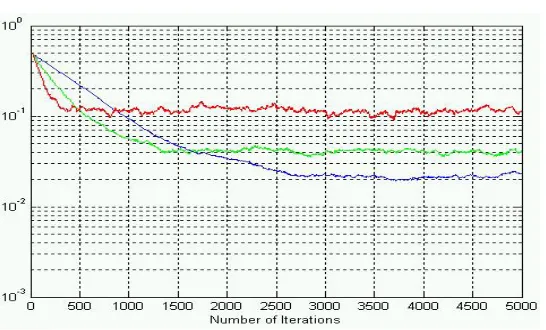
2.2.4 Step Size Parameter µ

Apparently, the convergence rate and misadjustment (or asymptotic performance) of the LMS algorithm are directly dependent on the step size parameter µ used in the tap weight adaptation formula (2-28). When the step-size parameter increases, the LMS algorithm converges faster with a larger final misadjustment (or worse asymptotic performance). Similarly, when the step-size parameter decreases, the LMS algorithm converges slower with a smaller final misadjustment (or better asymptotic performance). The behaviour of varying the step-size is illustrated in Figure 2.4.

µ = 0.005

µ = 0.002

µ = 0.001

Fig 2.4: Illustration on the Effect of Varying Step Sizes

In addition, to ensure the stability (or convergent) of the LMS algorithm, the step-size parameter is bounded by the following equation [1]:

0 < µ < ………

2.29 where tap-input power is the sum of the mean-squared values of all the tap inputs in the transversal filter and is given by

E |x n_k |

2.2.5 Effect of Filter Tap Length

Vol. 2(11), 2010, 6391-6407 convergence rates when the input signals are highly auto correlated [10].

2.2.6 Effect of Input Signal Power

The correction term µe(n)x(n) in LMS tap-weight adaptation is directly proportional to the tap input x(n). In other words, the convergence rate and stability of the LMS algorithm is directly dependent on the value of µσ2_x, where σ2_{x is the variance or power of the input signal [10].}

When the power of the input signal x(n) is large or varies greatly, the LMS algorithm demonstrates an unstable behavior known as gradient noise amplification. Consequently, the LMS algorithm becomes unstable and therefore will not lead to the optimal solution. To deal with this problem, a modified version of the LMS algorithm, also known as Normalized LMS, is implemented here

3. Normalized least Mean Square Algorithm

In many adaptive filter algorithms Normalized least mean square algorithm (NLMS) is also derived from conventional LMS algorithm. The objective of the alternative LMS-based algorithms is either to reduce computational complexity or convergence time. The normalized LMS, (NLMS), algorithm utilizes a variable convergence factor that minimizes the instantaneous error. Such a convergence factor usually reduces the convergence time but increases the misadjustment. In order to improve the convergence rate the updating equation of the conventional LMS algorithm can be employed variable convergence factor

μ

As noted in previous section, the value of µσ2

x directly affects the convergence rate and stability of the LMS adaptive filter. As the name may imply, the NLMS algorithm is an effective approach to overcome this dependence, particularly when the variation of input signal power is large, by normalizing the update step-size with an estimate of the input signal variance, σ2

x(n) [10]. In practice, the correction term applied to the estimated tap-weight vector w(n) at the n-th iteration is ‘normalized’ with respect to the squared Euclidean norm of the tap input x(n) at the (n-1)-th iteration [8],

w(n+1) = w(n) +

e n x n

Apparently, the convergence rate of the NLMS algorithm is directly proportional to the NLMS adaptation constant

µ, i.e. the NLMS algorithm is independent of the input signal power. Theoretically, by choosing µ so as to

Indeed as reported in [11], by taking into account the variation of signal level at the filter input and selecting a normalized correction term, we get a stable as well as a potentially faster converging adaptation algorithm for both uncorrelated and correlated input signal. It has also been stated that the NLMS is convergent in the mean square if the adaptation constant û (note that it is no longer called the step size) satisfies the following condition [12]:

0<

μ

Despite this particular edge that NLMS exhibits, it does have a slight problem of its own. Consider the case when the input vector x(n) is small. Instability may occur since we are trying to perform numerical division by a small value of the Euclidean Norm x(n) 2_.

However, this can be easily overcome [8] by appending a positive constant to the denominator in (2-28) such that

where is the normalization factor. With this, we obtain a more robust and reliable implementation of the NLMS algorithm.

In summary, we can write the LMS algorithm for every search iteration, in the form of three operations: Initial Condition: 0 < µ ̃≤ 2

x(0) = w (0) = [0, ……, 0]T _, c = a small constant

1. Filter Output: y(n) = w(n) x' (n) 2. Error Estimation: e(n) = d(n) - y(n)

3. Tap-weight adaptation: w(n + 1) = w(n) +

µ

4. DETAILED DESIGN AND IMPLEMENTATION

The LMS algorithm is a widely used adaptive algorithm which was developed by Windrow and Hoff in 1959[1]. It is based on the estimation of the gradient toward the optimal solution using the statistical properties of the input signal. Simplicity is the key feature of LMS algorithm. In this algorithm filter weights are updated with each new sample as required to meet the desired output.

Due to good convergence rate and stability the NLMS replaced the LMS adaptive algorithm. It has fast convergence rate compared to other adaptive algorithms which makes it to use in vast applications.

The below block diagram (figure 4.1)shows the inputs and outputs of the NLMS algorithm. It has four inputs and two outputs. Inputs are x_in (input data to adaptive filter),d_in (desired input), clk(clock) and adpt_enable (input bit used for ………). Outputs are error_out (difference between output of filter(y-out) and desired input (d_in) ) and final out (…).

The inputs x_in and d_in and outputs error_out and final_out are 8bit data.clock and adpt_enable are single bit data.

The NLMS block consists of two shift registers, calculator, adder and a multiplexer. The inner structure of the NLMS is as shown in figure 4.2 below

Fig.4.1: Input and output of NLMS Adaptive Algorithm

.

x in

d in

adpt enab

clk

final_ou

error o

Vol. 2(11), 2010, 6391-6407

Fig.4.2: Inner Structure of NLMS

The above block shows the inner structure of arrangements of the internal blocks of NLMS. Here the input to the adaptive filter x_in is given to the 20-bit shift register and desired input d_in is given to the 21-bit shift register. The two outputs of the 21-bit shift register are given to the calculator block which generates the output y_out. The output of the 20-bit shift register is subtracted with the output of calculator y_out. The subtracted output is given to the multiplexer where the enable bit is used as a select line. The other input of the multiplexer is “00000000”.

The calculator block is used for calculation of y_out at several iterations. Here we used for five iterations. We can call the calculator block as the core filter block because it generates the filter output y_out.

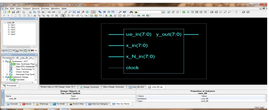
When we considering the calculator block as main block which is used for several iterations, it consist of five inputs and four outputs. In which only clock is the single bit input, all others are 8-bit data. The calculator block is as shown in figure 4.3.

y_ou

error_ou

Calculator

(Core filter)

clk

d in

21-bit shift

register

adpt enab

mu

cl

clk

X_i

20-bit shift

register

“000000

E

Y

Fig.4.3: Block Diagram of Calculator

.

The inputs of core_filter are assigned to different sub-blocks of it. Outputs of core_filter are used as the inputs for next iterations. At last iteration only y_out is considered as the output of the core_filter.

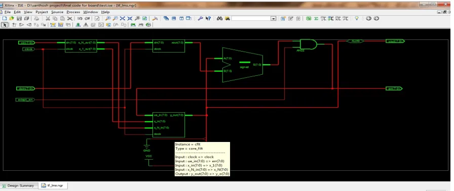
The inner structure of the core filter block is as shown in fig 4.4. As mentioned above the unit calculator is used 5 times in single core filter for the calculation of y_out. the other outputs are left open which are of no use.

Fig 4.4: Inner Structure of the NLMS Core Filter.

The calculator block has several internal blocks which performs the different arithmetic operations inside it.

Calculator

(Core filter)

x in

x N in

y in

clock

ue in

x out

X N out

ue out

Vol. 2(11), 2010, 6391-6407 The different blocks inside the core_filter are adder, multiplier, shift register, saturation, scaling, and truncation. The single calculator block uses some signals which are used for the calculation. The signals are shiftx(32), shiftxn(32), shiftue(24), shifty(16), coeff16(16), coeff8(8), xnin_ue(16), xnin_ue_scaled(16), new_coeff (16), delayed_new_coeff (16), y_out16(16) and y_out8(8). The numbers in bracket refers to the bit size of that signal.These signals are used during the different arithmetic operation of the input data at the calculator block.

The first block of the calculator is multiplier which multiplies the 8bit datas x_N_in and ue_in. the output signal xnin_ue is 16bit data. The second stage is scaling. In scaling stage the out may be upgrade or degrade of the input signal. Here we always degrade the output of the multiplier stage. The output is xnin_ue_scaled is also 16-bit, which is added to the 16-bit co-efficient signal coeff16 at next stage. The signal new_coeff is the outputof the adder stage which is delayed by using shift register in next step. The delayed new coefficient which is the output of shift block is 16-bit data which is used in calculation of the next coefficient for core filter. The output checked for its limit in saturation stage. In saturation stage care is taken about the data not to exceed the limit of the coefficient. The saturated data is truncated to 8-bit in next stage.

The next stage is 8bit multiplier which multiplies the 8bit truncated coefficient with 8MSB bits of shiftx signal which gives 16-bit product. These 16 bit output i.e y_out 16 is truncated to 8-bit in next stage. The 8-bit output is the final output of the core_filter after 5th _iterations.

5. System Identification

System identification is one of the most interesting applications for adaptive filters, especially for the Normalized Least Mean Square algorithm, due to its convergence rate, robustness and calculus simplicity. Based on the error signal, the filter’s coefficients are updated and corrected, in order to adapt, so the output signal has the same values as the reference signal. The application enables remarkable developments and research, creating an opportunity for automation and prediction.

Identifying an unknown system has been a central issue in various application areas such as control, channel equalization, echo cancellation in communication networks and teleconferencing etc. Identification is the procedure of specifying the unknown model in terms of the available experimental evidence, that is, a set of measurements of the input-output desired response signals and an appropriately error that is optimized with respect to unknown model parameters. Adaptive identification refers to a particular procedure where we learn more about the model as each new pair of measurements is received and we update the knowledge to incorporate the newly received information.

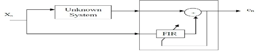
System identification refers to the ability of an adaptive system to find the FIR filter that best reproduces the response of another system, whose frequency response is a priori unknown. The set up is shown in fig 5.1:

Fig 5.1: System Identification using Adaptive Filter.

When the adaptive system reaches its optimum value and the output (e) is zero an FIR filter is obtained whose

6. SYNTHESIS AND SIMULATION RESULTS

The implemented VHDL program for NLMS adaptive algorithm is now synthesised using Xilinx 10.1. Modelsim is used to study the waveforms of each stage. The VHDL programs are synthesised separately for each block. The synthesis result observed for core filter of the NLMS block and the total NLMS block separately are shown below.

6.1core filter

Fig 6.1: Top Module of Core Filter

.

Vol. 2(11), 2010, 6391-6407

Fig 6.3: Internal Structure of the Core Filter (final tap).

Fig 6.5: Modelsim output of Core Filter.

Vol. 2(11), 2010, 6391-6407

Fig 6.7 Inner Structure of NLMS

Fig 6.8 Modelsim output of NLM

7. Conclusion

Adaptive Digital Signal Processing is a specialized branch of DSP, dealing with adaptive filters and system design. There are number of adaptive algorithms available in literature and every algorithm has its own properties, but aim of every algorithm is to achieve minimum mean square error at a higher rate of convergence with lesser complexity.

In this paper , we focused on system identification using NLMS-based FIR adaptive filter. The key reasons for selecting NLMS as the adaptive algorithm are:

° Simplicity i.e. low computational cost and ease of implementation ° Robust and Reliable

Our approach to the ultimate goal began by identifying the causes behind the problems that leads to performance degradation in using conventional LMS algorithm. Then we deployed existing techniques and methods to tackle each problem separately. Finally, we observed how each of these techniques can work for each other and proposed a solution in which all the problems can be resolved as a whole.

A review of adaptive filters shows that the NLMS algorithm is still a popular choice for its stable performance and high-speed capability. The other advantage of the NLMS over other adaptive algorithm is its high convergence rate.

The high-speed capability and register rich architecture of the FPGA is ideal for implementing NLMS. A hybrid adaptive filter is designed with a direct-form FIR filter coded in VHDL and with the NLMS algorithm written in VHDL code executing on the Xilinx.

8. REFERENCES

[1]. B. Widrow and S.D.Stearns,” Adaptive Signal Processing”, Prentice-Hall, Englewood Cliffs, N.J., 1985.

[2]. S. Haykin, “Adaptive Filter Theory”, Fourth Edition, Prentice Hall, Upper Saddle River, N.J., 2002.

[3]. Choo, P. Padmanabhan, S. Mutsuddy, ,,An Embedded Adaptive Filtering System on FPGA”, Department of Electrical Engineering, San Jose State University, CA 95198- 0084 USA.

[4]. Scott C. Douglas, “Analysis of the Multiple-Error and Block Least-Mean-Square Adaptive algorithms”, IEEE Transactions on Circuits and

Systems – II: Analog and Digital Signal Processing, Vol 42, No. 2, p. 92, February 1995.

[5]. Lattice Semiconductor Corporation, “LMS Adaptive Filter”, Reference Design RD1031, December 2006.

[6]. Sinead Mullins, Conor Heneghan, “Alternative Least Mean Square Adaptive Filter Architectures for Implementation on Field Programmable

Gate Arrays”, Digital Signal Processing Group, Department of Electronic and Electrical Engineering, University College Dublin.

[7]. Ahmed Elhossini, Shawki Areibi, Robert Dony, “An FPGA Implementation of the LMS Adaptive Filter for Audio Processing”, IEEE

International Conference on Reconfigurable Computing and FPGA's, ReConFig 2006 ,ISBN: 1-4244-0690-0.

[8]. S. Haykin, Adaptive Filter Theory, Prentice Hall, New Jersey, 1996.

[9]. B. Farhang-Boroujeny, Adaptive Filters: Theory and Applications, John Wiley & Sons, West Sussex, England, 1998.

[10]. J. Homer, —Adaptive Echo Cancellation in Telecommunications“, Ph.D. dissertation, The Australian National University, Canberra, April 1994.

[11]. S.C. Douglas and T.H.-Y. Meng, —Normalized Data Non-linearities for LMS Adaptation“, IEEE Transactions on Acoustics Speech Signal Process, vol. 42, pp 1352-1365, 1994.

[12]. T.C. Hsia, —Convergence Analysis of LMS and NLMS Adaptive Algorithms“, Proceedings for ICASSP, Boston, Mass., pp 667-670, 1983. [13]. HDL CHIP DESIGN by Douglas J Smith, 1997 Edition.

[14]. D.Gajaski and R. Khun, “Introduction: New VLSI Tools”, IEEE Computer, volume 16, Dec 1983. [15]. Digital System Design Using VHDL by Charles H Roth, Jr PWS Publication Company 1998 Edition. [16]. Circuit Design with VHDL by Volnki A.Pedroni, MIT Press 2004, PP 3-4.

[17]. A Modified Least Mean Square Algorithm Using Fractional Derivative and its Application to System Identification,Raja Muhammad Asif Zahoor, International Islamic University, Ijaz Mansoor Qureshi, Air University, Pakistan, Vol.35 No.1 (2009), pp 14-21 Euro Journals Publishing, Inc. 2009.