S
S
S
e
e
e
n
n
n
s
s
s
o
o
o
r
r
r
s
s
s
&
&
&
T
T
T
r
r
r
a
a
a
n
n
n
s
s
s
d
d
d
u
u
u
c
c
c
e
e
e
r
r
r
s
s
s
ISSN 1726-5479
© 2009 by IFSA
http://www.sensorsportal.com
A Bayesian Approach to Solving the Non – Invasive Time
Domain Reflectometry Inverse Problem
Ian G. PLATT and Ian M. WOODHEAD
Lincoln Ventures, PO Box 133, Lincoln, Christchurch 7640, New Zealand Tel.: +64 3 325 3748, fax: +64 3 325 3725
E-mail: [email protected]
Received: 10 July 2009 /Accepted: 31July 2009 /Published: 10 August 2009
Abstract: Non Invasive Time Domain Reflectometry (TDR) may be used to estimate the volumetric
moisture content, θv, with depth for a variety of sample materials. The forward physical model is couched in terms of a moment method where integration is performed over a descretized sample space to estimate the measured propagation time tp down a pair of parallel transmission lines. We show that
the inverse solution to this, which recovers relative permittivity and thus θv, is greatly facilitated by a simplification of the system geometry via, 1) realistically modeling the prior density of the sample, 2) using this prior with the inherent system symmetry to reduce the number of required discretization cells, and 3) determining a physically meaningful reduction operator to allow a coarse discretization mesh to be used. The observational equation is expressed in the Bayesian paradigm with the most accurate and robust solution obtained using the Conditional Mean of the posterior distribution constructed via a Monte Carlo method. Results of simulation show that the method is capable of providing accurate estimates of the moisture density profile down to a depth of 100 mm with an error of less than 4 %. Further, the reduction in the number of descretized cells required to accurately estimate these profiles means that the inversion procedure is quick enough to enable the real time application of the equipment, a fundamental requirement in the development. Copyright © 2009 IFSA.
Keywords: Time domain reflectometry, Bayesian, Non invasive, Moisture content, Transmission
lines, Electromagnetic sensor
1. Introduction
Three basic methods have been developed over this period, namely; gravimetric, neutron scattering and electromagnetic [1], [2]. Gravimetric methods are accurate but have the disadvantage that the sample must be removed, while neutron scattering sensors must be closely monitored and cannot be left unattended, since they pose a health risk. The role of electromagnetic sensors, which suffers neither of these disadvantages, has thus become of increasing importance for soil moisture content measurement. Most of the current electromagnetic systems estimate the relative permittivity, εr, of the sample by deploying two or more metallic probes into the soil to measure the capacitance or impedance between them, or as in the case Time Domain Reflectometry (TDR), the time delay of a pulse sent down a pair of probes acting as a transmission line. The εr of the sample is then related to its volumetric moisture content, θv by an empirical relationship such as those derived by [3] and [4]. Since water has a high relative permittivity, εr 80, compared to values of εr ≤ 5 for most other components that make up typical samples the pulses velocity change is most sensitive to the amount of water present. The measured permittivity can be related to the samples dielectric properties by a real part representing the stored energy of the system and an imaginary part describing its energy dissipation:
, (1)
where is the stored energy of the system, is the electrical conductivity between the probes, is the molecular relaxation of the water molecules and is the frequency of the probe signal.
In this work we assume a lossless media so that the imaginary part of (1) becomes negligible and the effective permittivity for the system is . In those cases where this is not justifiable [5] have developed a method whereby allowance for the conductivity part of the loss can be easily incorporated.
For the invasive TDR system a pair of parallel transmission lines are inserted into the sample and a short pulse is sent down them generating a static electric field. This field causes the sample dielectric to produce an opposing polarization field that reduces the phase velocity of the pulse. The velocity of the pulse can be given in terms of the permittivity and permeability of the sample by:
, (2)
where is the relative permittivity, c is the speed of light and is the relative permeability
(which is equal to one for most soils). By measuring the time the pulse takes to travel down the transmission line of length, d, and back again after a reflection from the end, the propagation time can
be related to from (2) (with ) by:
(3)
Woodhead [6] extended this TDR arrangement by deploying the transmission lines external to the
(4)
This equation represents the forward construction of the physical system where the form of is specified in section 2. Since we seek an estimate of from a measured value of it is the inverse of this equation that is required:
(5)
In common with many other inverse problems, the solution of (5) is somewhat problematic. The forward function is both non-linear and ill-conditioned thus an estimate of by the inverse process requires some form of regularized optimization technique. Further, since no analytic solution to the forward model is available, the method of moments technique in which the sample is discretised, is used as an approximation to the solution. The level of discretisation, or mesh size, will of course have an effect upon the accuracy of this approximation.
The objective of this paper is to describe a methodology for improving the accuracy and efficiency of the inverse defined by (5) via a Monte Carlo simulation.
2. Background
The steps in defining the function f in the forward model of (4) are derived by Woodhead [6] which we
briefly recount here. When an incident electric field, is imposed upon a dielectric of volume , the dipole moment P, of the volume produces an electric field, . The total electric field is then:
(6)
Using the constitutive relationship this becomes, after some re-arrangement:
, (7)
where is the permittivity of free space and is the relative permittivity of the dielectric. may be calculated at a point r from the polarization element P via:
(8)
So that (7) becomes:
(9)
and this may be expressed in terms of a linear operator, L, acting upon P, [10] as:
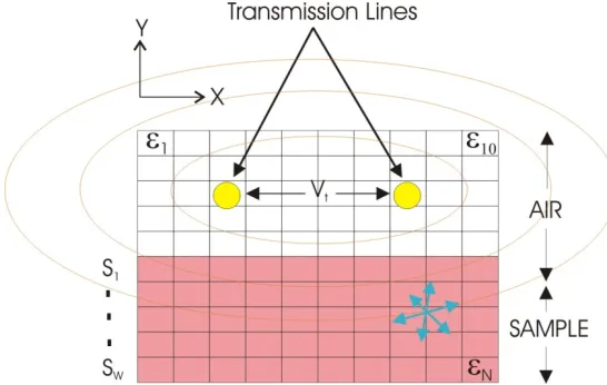
Upon discretisation into N cells, as depicted in Fig. 1, the polarization field of (8) becomes:
(11)
where m is the cell at which the polarization field from cell n (source cell) is to be calculated. Since, by
model assumption, the z-component is constant, expanding over the gradient function gives:
,
(12)
where and are the x and y differences between the points m and n respectively. Note that
when m = n (i.e. the cells own polarization field) components become:
(13)
By using the method of moments with a subsectional basis function defined as non zero only for the source cell, Harrington [10] showed that (10) can be written in the discrete matrix form:
(14)
with the components of L given by the square bracketed part of (12) for and by
(15)
when , where . Since both L and P are functions of the independent variable, (14) is non-linear.
Woodhead [6] extended the discretised model of (14) by introducing the concept of a transmission line
to produce the incident field , so that the pulse velocity, v, due to the dielectric interaction can be
given by the telegraphers equation (e.g. [11]):
(16)
so that
where is the total voltage between the transmission lines, is the component due to the polarization field induced by the dielectric sample and is the component due to the incident electric field directly from the transmission lines; d is the length of the transmission line; is the propagation
time of the pulse from the beginning of the line to its reflection at the end and back to the beginning;
ρ is the line charge density; µ is the magnetic permeability; b is the spacing between the parallel lines,
and a is the diameter of the transmission lines.
The only unknown on the right hand side of (17) is the polarization induced voltage, , contained in the total voltage Equation (17) may thus be succinctly represented by:
(18)
Following the method of [7] both the transmission lines and sample can be imbedded in the discretisation space, depicted by Fig. 1, so that:
, (19)
where M is the number of cells between the transmission lines and w is the width of the cell.
Fig. 1. The 2D geometry of discrete cells and parallel transmission lines used to define the system matrix equation. The cells between the transmission lines are those (M of them) included
in the calculation of . Each of the cells has a width w.
For any particular value of permittivity in each sample cell, the polarization P within it can be calculated from (14) since so for those cells:
, (20)
(21)
The forward solution defined by (4) can now be formed by the composition of the two functions Ψ and
Φ so that:
(22)
3. Bayesian Formulation
In exploring the solution to the inverse problem outlined by (4) we use the Bayesian framework as described for example by [8] and [9]. In this representation (4) may be written in the observational form as:
, (23)
where now T and F represent the random variables (with and as realizations) and we have
added as the measurement noise, assumed to be independent of F. An inverse solution to this
equation can be given in terms of the variable densities by the well know Bayes Formula:
, (24)
where is the posterior density, is the likelihood density function and is the prior density function of the permittivity and will act as a regularization for different physical assumptions about the likely structural disposition of throughout the sample. The term , often called the evidence factor, can be viewed as a scaling factor that ensures a unit total probability of the posterior density function. Since it plays no part in the evaluation of the required parameters of the posterior distribution it is usually ignored so that the above equation becomes:
(25)
To obtain an estimate of corresponding to the measurement we can use either the Maximum A Posteriori Estimator (MAP) or Conditional Mean (CM) of the posterior distribution given by (25), with associated errors given by the covariance . Both the CM and estimates require integration over the posterior density :
(26)
with the estimate error given by the posterior covariance
(27)
while the MAP estimate:
is usually achieved by some sort of optimization method.
The construction of the applicable form of (25) for the TDR model will be detailed in section 3.4 after some relevant properties of the system (such as parameter independence) are established.
3.1. Required Level of Discretisation
In the observational model of (23), T is the measured value of the propagation time, with realization
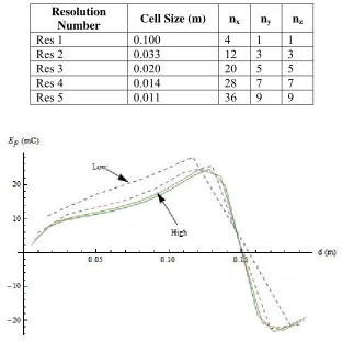
. Since no measurements are available, model validation must be carried out using simulated data which should be generated at a high enough level of resolution that it is as close as possible to the perceived real case. For this case we content ourselves with a level of discretisation that provides a model accuracy that cannot be much improved upon by further decreases in mesh size. To determine this level of discretisation, the polarization electric field, , between the transmission lines was calculated using (22) for an increasing number of individual cells over a constant sample volume. The results of this are shown in Fig. 2. Here the polarization field converges to that given by the mesh sizes of Res 4 (defined in Table 1).
Table 1. Discretisation values. nx, ny, nz, are the number of cells in the directions x, y and z respectively.
Resolution
Number Cell Size (m) nx ny nz
Res 1 0.100 4 1 1
Res 2 0.033 12 3 3
Res 3 0.020 20 5 5
Res 4 0.014 28 7 7
Res 5 0.011 36 9 9
Fig. 2. The polarization field distribution over the half plane between the transmission lines. Each of the
curves represents a different Resolution, defined by Table 1, for a constant volume sample.
calculations and will be used in section 3.4 to construct a resolution reduction operator q and in section
4 to test the inversion procedure.
3.2. Operational Discretisation
In the previous section we established that the discretisation level, labeled as Res 4 of Fig. 2 and Table 1, provided the closest accessible level of mesh size that could represent the true environment. Computation at this level of discretisation is very slow however and certainly unacceptable for the real time applications required for the TDR. Even the pre-calculation of much of the Monte Carlo sampling described in [12] would be impractical at this level. It would therefore be advantageous to perform the calculations in the coarser mesh of Res 2, and then use a map Q to project the results into those that
would have resulted from the finer mesh:
, (29)
where the high resolution (Res 4) and low resolution (Res 2) are represented by the subscripts h and l
respectively. The observational equation (23) for the high resolution, Res 4, can be written in this terminology as:
, (30)
where is the propagation time and is the measurement noise. Applying the operator, Q, this
becomes:
(31)
with
(32)
being the error introduced by using the coarser discretisation. In this sense the operator Q can be
termed as the model reduction operator [8]. Putting the total error as:
; (33)
the equation (31) can be written as:
, (34)
where we have made the assumption throughout this formulation that the discretisation error is approximately independent of the relative permittivity, . This is discussed in more detail in section 3.4.
With the propagation time measurement and the form of the likelihood function becomes:
, (35)
given by the combined error of (33). If the distribution is close to Gaussian, which is often the case, [9] shows that the above equation becomes:
, (36)
where and are the expectation and covariance respectively of the total error distribution, . Here the mutual dependence of and the approximation error have been ignored, a simplification that will be addressed further in the next section.
The values of can be pre-calculated because of the unique system geometry and operational constraints [12], so once the operator q is known the calculation speed of (35) is acceptable for real
time application. The required posterior density is thus:
(37)
3.3. Prior Densities
As discussed in [12] for many cases of practical interest the moisture within the sample can be considered as being stratified in the x -z plane. Apart from reducing the number of unknown permittivity values to be calculated, plane stratification also leads to symmetry in the x - z plane that can be utilized to decrease the number of dimensions of the inverse system. In keeping with this stratified geometry of the sample we define three prior distributions for , each representative of a number of real world scenarios. In the first case, the prior is given as a positive increase in relative permittivity with depth. With the discretisation level of Res 4 it can be defined as:
, (38)
where , is the uniform distribution and .
The second prior is similarly defined but with a decrease in permittivity with depth, so that the incremental permittivity between layers is defined by . For both of these distributions the maximum change of over the sample depth is 14. A third prior is included as a subset of the first, that of a positive linear gradient over the sample. In this case the value of the upper boundary of the sample is chosen from the distribution , while the lower sample boundary value is chosen from . for the centre of each depth layer is then obtained by linear interpolation. Each of these will be used in the examples that follow.
3.4. Mapping Operator
After defining the form of the next immediate concern is to find a model reduction operator Q
that maximizes the decrease of in (32) and thus in (37). For such an operator to be useful it must be only weakly dependant on the actual sample relative permittivity .
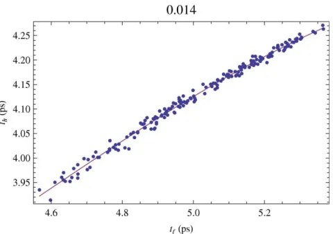
interpolation over the midpoints of the seven Res 4 cells. The Fig. 3 shows the relationship between the two propagation times for the transmission line height above the sample of . A good fit to the data for each height in this figure is achieved by the polynomial:
(39)
where a, b and c are chosen for each of the different heights. In terms of the Bayesian paradigm of (37) then:
(40)
Values of the coefficients for this polynomial are easily calculated by any of the standard fitting routines and are applicable to all measurements with the same geometrical relationships and prior relative permittivity distributions. The form of (40) is also a valid approximation for the reduction operator when the other prior distributions defined in section 3.3 are used, though the coefficients at similar heights may differ.
Fig. 3. The form of the projection operator Q between the low resolution and high resolution discretisation models for a transmission line heights = 0.014 m above the sample. and are the propagation times for
Res 2 and Res 4 respectively. Other heights above the sample give a similar relationship.
Table 2 shows the standard deviation, , of data difference from the fitted polynomial for the different priors discussed above. These values can be used for defining the distribution in (33) and together with the measurement noise , constitute the total error, from which the covariance, of (37) is extracted. The mean error in all fitted cases is zero and since we have . Further, the low dependence of the discretisation error on shown explicitly in Fig. 3, strengthens the ability of the enhanced error model of (37) to represent the real situation.
Table 2. The standard deviation, , of data fitted to (40) for the indicated transmission line heights.
Given in ps ( ).
30.0 13.7 7.6 27.8 10.5 5.6
Using from Table 2 and from previous experimental work [12], the Gaussian distributions and can be defined for (33). The errors are dependent upon the current transmission line height only, so:
(41)
is a diagonal matrix containing the total error variance for each height. Re-writing (37) with and the covariance gives the form of the posterior density used in subsequent simulations as:
(42)
Thus the posterior distribution of can be generated with the computationally accessible Res 2. From this distribution an estimate of for each layer can made from the CM of (26) with its associated error estimate given by the covariance defined by (27).
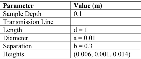
Table 3. System parameters
Parameter Value (m)
Sample Depth 0.1 Transmission Line
Length d = 1
Diameter a = 0.01
Separation b = 0.3
Heights (0.006, 0.001, 0.014)
3.5. Some Practical Simplification for Computation
The posterior distribution may be generated by the Monte Carlo approach described by [12] with an estimate for its value given by the CM. Although in this scheme much of the likelihood function is pre-calculated using (22), the large number of calculations required together with possible real time refinements results in a heavy computational burden for the required level of discretisation. To reduce the computational effort to something manageable the previous sections looked at reducing the number of dimensions of the observational form. Another purely physical reduction in complexity can be achieved by simplifying the geometry represented in Fig. 1.
The geometry depicted in Fig. 1 indicates that a potentially large number of cells represent air, with a known permittivity of . These cells, apart from those between the transmission lines, provide no extra information and can be discarded. Removing these cells from the model the polarization of the sample cells may now be related to those cells between the transmission lines by a gradient function similar to that given by the bracketed terms of (12) ([12]). If G is this gradient function, then the
polarization in each sample cell ( ) may be related to the field between the transmission lines ( ) by:
(43)
, (44)
where and L now refer only to the sample cells.
As discussed in [12] for many cases of practical interest the moisture within the sample can be considered as being stratified in the x -z plane. Apart from reducing the number of unknown permittivity values to be calculated, plane stratification can again also lead to a further simplification in the specification of the forward model. Fig. 4 represents a sample material with N cells and
consequently N unknown values of permittivity. By assuming plane stratification the number of
unknown permittivities is reduced to the number of stratum (5 in the example of Fig. 4). In theory if there are N unknown values of permittivity there must be N independent measurements of the
propagation time, . For example, for five stratums each having an unknown value of , five measurements of are required to specify the system of equations represented by Error! Reference source not found.. To generate an independent set of components, each measurement of is made at
a different height of the transmission lines above the sample. From this argument it is clear that the planar stratification also decreases the number of required measurements.
Fig. 4. Physical geometry of the TDR system. Because of the form of the gradient field, it is essential that the centers of the cells between the lines are aligned with those of the sample.
Another important simplification in the geometry can be made by considering the symmetry of the system. The component values of the entire samples polarization and their effect on between the transmission lines can be represented by a reflection of the shaded quarter space shown in Fig. 4. Hence, by avoiding duplication of symmetric cells, it is possible to further reduce the components of L, G and by a factor of four.
4. Results
Having formulated a solution to the operational objectives outlined in the Introduction it remains to show how well it performs. Since this is a simulation, it is sensible to test the operational procedure by using the high resolution and computationally intensive (Res 4) simulated values to represent the “real world” instantiation of the TDR system and measurement.
These parameters remain constant throughout all simulations (including those of the previous section) in this paper.
4.1. Relative Permittivity Profiles
Random values of were assigned to each one of the 7 depth layers defined by Res 4, according to the prior scenarios depicted in Table 2. Using (4), the simulated (or measured) value for was then calculated at each transmission line height. Using the appropriate value for the reduction operator, q,
and the Monte Carlo procedure detailed in [12] for the lower resolution , the posterior density of (42) was generated. An estimate for was then determined from the CM of (26) and compared with the original values. Since Res 4 has 7 layers its profile is linearly interpolated to the cell centers of the Res 2 case for this comparison.
Table 4 shows the standard deviation of the difference between the simulated and estimated value of for 200 cases of each prior scenario. The standard deviation for each case is small compared to the range of covered and is well within requirements for practical use, where volumetric moisture content is to be estimated (next section). Note that there is a small decrease in the error as the prior distribution is more tightly constrained (i.e. between the more flexible uniform distribution profiles and the constrained linear profile).
Table 4. Standard Deviation, , of the difference between the estimated and simulated values of .
Layer Depth (m) linear
1 0.016 0.46 0.43 0.21 2 0.050 0.45 0.46 0.34 3 0.066 0.74 0.65 0.65
Note, because is Gaussian with mean and a large number of samples are used, one can either use the form of the likelihood function in (42) or the simplified version taking into account only the measurement noise variance , to obtain the statistics on the error in determining . In the following, the form of (42) is used since it is the most general.
4.2. Moisture Profiles
The object of the TDR method is to measure the moisture content profile of a sample with depth. The inverse methodology discussed previously has focused upon relative permittivity since the mapping from this to a moisture estimate is straightforward and can be applied after the inversion procedure. Topp [3] showed that this mapping could be described by:
, (45)
where is the volumetric moisture content.
this example is close to the maximum variation expected. From the original profile, values corresponding to the cell centers of the fine mesh are taken and converted to the corresponding via interpolation of Error! Reference source not found.. These values are then used for the Res 4
permittivity profile to generate the simulated observations, , after which the method described in the previous section is used to estimate the value of with the reduced system calculations. The estimates, returned to volumetric moisture via Error! Reference source not found. are also shown in
Fig. 5a. A second example is given in Fig. 5b where the moisture content nears field capacity at the surface and dries out with depth, a situation during heavy rain. Both examples show a good reconstruction of the moisture profile, albeit at the lower depth resolution corresponding to the 3 layer discretisation of Res 2. Also shown on both figures are the MAP estimates of for the three coarse mesh layers, using the same Monte Carlo data. Their poor ability to reconstruct the simulated curve indicates that a minimization procedure would require further real time processing (e.g. extended distribution sampling using some form Markov chain Monte Carlo method). There seems little to be gained from pursuing this path at present.
(a) (b)
Fig. 5. (a) Simulated depth profile for the percentage volumetric moisture content, of a soil sample. The
form of the moisture distribution with depth follows the prior distribution of permittivity given by
between layers. Physically this corresponds to a loamy soil drying near the surface. The solid line is the original model for the moisture content depth profile, while the ▲ are the points chosen for the midpoint of the 7 layer Res4 representation. The CM and MAP estimates of the inverse in Res 2 are shown as and ³ respectively. (b) Similar but with a permittivity prior of between the layers. The physical situation represents moisture content near field capacity at the surface and drying with depth. The CM estimate is shown by . Note that only one MAP estimate ³) is within the plot range.
In more general terms than the examples above, the expected error in volumetric moisture content, , can be derived from applying of Table 4 to the differential of Error! Reference source not found.:
(46)
5. Conclusion and Discussion
The aim of this work has been to simplify the TDR inversion model so that its real time application can be achieved. To this end we have decomposed the original model into a reduced set of cells by exploiting both planar geometry and system symmetry. This together with the likely distribution of moisture content with depth provided a powerful prior model for the inverse process defined in a Bayesian framework. The level of discretisation required to avoid errors through the discretisation itself has been determined to be given by a cell size of 0.014 m for the proposed operational system geometry. Since this level of discretisation is impractical for operational use, an effective reduction operator has been developed that allows the TDR inversion procedure to be carried out at a much coarser mesh level (a cell size of 0.0333 m). Further, the use of this reduction operator produces a relatively small error in the CM estimate of the relative permittivity in the layered sample. With the Monte Carlo approach previously developed [12], the inversion is easily accommodated within a time scale and accuracy suitable for “in the field” use of the TDR equipment. As pointed out, many practical samples do not have a rapidly changing permittivity (or direction of gradient) over the 100 mm or so of depth, so for many practical purposes the prior scenarios studied are appropriate.
In practice there are a number of considerations to be assessed when applying the procedure described here to an operational system. These include the dependence of the reduction operator on the moisture (or relative permittivity) profile and improving the representation of the electric field within the method of moments formalism. [13] discusses these issues more fully.
References
[1]. K. Noborio, Measurement of soil water content and electrical conductivity by time domain reflectometry: a review, Computers and Electronics in Agriculture, Vol. 31, 2001, pp. 213-237.
[2]. S. R. Evett and G. W. Parkin, Advances in Soil Water Content Sensing: The Continuing Maturation of Technology and Theory, Vadose Zone J., Vol. 4, 2005, pp. 986-991.
[3]. G. Topp, State of the art measuring soil water content, Hydrological Processes, Vol. 17, 2003, pp. 2993-2996.
[4]. J. Ledieu, P. De Ridder, P. De Clerck and S. Dautrbande, A method of measuring soil moisture by time domain reflectometry, Journal of Hydrology, Vol. 88, 1986, pp. 319-328.
[5]. I. M. Woodhead, I. G. Platt, Pseudo-Static Electromagnetic Modelling of Moisture Sensors in Lossy Dielectrics, 7th Conference on Electromagnetic Wave Interaction with Water and Moist Substances, Hamamatsu, Japan, 2007.
[6]. I. M. Woodhead, G. Buchan and D. Kulasiri, Pseudo 3-D Moment Method for Rapid Calculation of Electric Field Distribution in a Low Loss Inhomogeneous Dielectric, IEEE Transactions on Antennas and Propagation Vol. 49, 2001, pp. 1117-1122.
[7]. I. M. Woodhead, G. Buchan, D. Kulasiri and J. Christie, A new model for the response of TDR to heterogeneous dielectrics, Subsurface Sensing Technologies and Applications, Vol. 1, 2000, pp. 473-487. [8]. J. Kaipio and E. Somersalo, Statistical and Computational Inverse Problems, Springer-Verlag, New York,
2005.
[9]. S. R. Arridge, et al., Approximation errors and model reduction with an application in optical diffusion tomography, Inverse Problems, Vol. 22, 2006, pp. 175-195.
[10]. R. F. Harrington, Field Computation by Moment Methods, R. E. Kreiger, 1987. [11]. W. C. Elmore and M. A. Heald, Physics of Waves, McGraw-Hill, NY, 1969.
[12]. I. G. Platt and I. M. Woodhead, A 1-D Inversion for Non-Invasive Time Domain Reflectometry, Meas. Sci. Technol., Vol. 19, 2008, pp. 055708.
[13]. I. G. Platt and I. M. Woodhead, Improving the resolution of Non-Invasive Time Domain Reflectometry, 3rd International Conference on Sensing Technology (ICST), 2008, pp. 224-233.
[14] R. G. McLaren and K. C. Cameron, Soil Science, Oxford University Press, 1990.
and Electrical Conductivity Measurement in Soils Using Time Domain Reflectometry, Vadose Zone J, Vol. 2, 2003, pp. 444-475.
[16]. Magnus Persson and Sahar Haridy, Estimating Water Content from Electrical Conductivity Measurements with Short Time-Domain Reflectometry Probes, Soil Sci Soc Am J, Vol. 67, 2003, pp. 478-482.
___________________