https://doi.org/10.5194/amt-12-4659-2019 © Author(s) 2019. This work is distributed under the Creative Commons Attribution 4.0 License.
Bayesian atmospheric tomography for detection and quantification
of methane emissions: application to data from the 2015
Ginninderra release experiment
Laura Cartwright1, Andrew Zammit-Mangion1, Sangeeta Bhatia2,a, Ivan Schroder3, Frances Phillips4, Trevor Coates5, Karita Negandhi6,b, Travis Naylor4, Martin Kennedy6, Steve Zegelin7, Nick Wokker8, Nicholas M. Deutscher4, and Andrew Feitz3
1School of Mathematics and Applied Statistics, University of Wollongong, Wollongong, Australia 2Centre for Research in Mathematics, Western Sydney University, Parramatta, Australia
3Geoscience Australia, Canberra, Australia
4Centre for Atmospheric Chemistry, School of Earth, Atmospheric and Life Sciences, University of Wollongong, Wollongong, Australia
5School of Agriculture and Food, University of Melbourne, Melbourne, Australia 6Department of Earth and Planetary Sciences, Macquarie University, Sydney, Australia 7CSIRO Oceans and Atmosphere, Canberra, Australia
8Department of Industry, Innovation and Science, Canberra, Australia acurrently at: School of Public Health, Imperial College London, London, UK bcurrently at: Office of Environment and Heritage, Parramatta, Australia
Correspondence:Laura Cartwright ([email protected]) Received: 29 March 2019 – Discussion started: 23 April 2019
Revised: 29 July 2019 – Accepted: 30 July 2019 – Published: 2 September 2019
Abstract. Detection and quantification of greenhouse-gas emissions is important for both compliance and environment conservation. However, despite several decades of active re-search, it remains predominantly an open problem, largely due to model errors and assumptions that appear at each stage of the inversion processing chain. In 2015, a controlled-release experiment headed by Geoscience Australia was car-ried out at the Ginninderra Controlled Release Facility, and a variety of instruments and methods were employed for quan-tifying the release rates of methane and carbon dioxide from a point source. This paper proposes a fully Bayesian ap-proach to atmospheric tomography for inferring the methane emission rate of this point source using data collected dur-ing the experiment from both point- and path-sampldur-ing in-struments. The Bayesian framework is designed to account for uncertainty in the parameterisations of measurements, the meteorological data, and the atmospheric model itself when performing inversion using Markov chain Monte Carlo (MCMC). We apply our framework to all instrument groups using measurements from two release-rate periods. We show
that the inversion framework is robust to instrument type and meteorological conditions. From all the inversions we con-ducted across the different instrument groups and release-rate periods, our worst-case median emission release-rate estimate was within 36 % of the true emission rate. Further, in the worst case, the closest limit of the 95 % credible interval to the true emission rate was within 11 % of this true value.
1 Introduction
have been conducted in order to improve techniques for estimating greenhouse-gas emissions (Flesch et al., 2004; Lewicki and Hilley, 2009; Loh et al., 2009; Etheridge et al., 2011; Humphries et al., 2012; van Leeuwen et al., 2013; Luhar et al., 2014; Jenkins et al., 2016; Ars et al., 2017). Building on this body of work, in 2015 a CH4 and CO2 controlled-release experiment was held at the Ginninderra Controlled Release Facility in Canberra, Australia (Feitz et al., 2018). This large multidisciplinary, multi-institutional blind-release trial (i.e. the participants did not know the true release rate) simultaneously assessed eight different CH4 emission-rate estimation techniques, using data from both mobile and stationary instrumentation. These eight techniques included tracer ratio techniques, backwards La-grangian stochastic modelling, forward LaLa-grangian stochas-tic modelling, Lagrangian stochasstochas-tic footprint modelling, and atmospheric tomography techniques. A full description of the methods and results is given in Feitz et al. (2018).
Every group involved in the analysis presented in Feitz et al. (2018) used a unique combination of instrumenta-tion and estimainstrumenta-tion technique when carrying out the anal-ysis, making it hard to establish the respective merits (or otherwise) of the employed techniques from the inversion results. Nonetheless, an interesting observation from the study is that none of the eight techniques deployed dur-ing the blind-release trial had a leakage uncertainty range (95 % interval) that included the true emission rate, while some estimates (including one obtained using atmospheric tomography) were factors of 2 or more off from the true value. Given that atmospheric methane concentration and meteorological instrument measurement uncertainty is gen-erally low for each of the different approaches, it suggests that the techniques that were used did not adequately ac-count for the variability of atmospheric measurements or the uncertainty introduced through parameterisation of at-mospheric mixing conditions (e.g. Monin–Obukhov lengths and/or Pasquill stability classes; see Sect. 3.1) and atmo-spheric dispersion/transport model uncertainty.
A number of studies have highlighted the importance of atmospheric-model error in estimating emission rates or fluxes (e.g. Chevallier et al., 2010; Basu et al., 2018). For example, Peylin et al. (2002) showed that flux estimates
transport model integrating weather research and forecasting into a Lagrangian particle dispersion model), which allows for quick simulation at various parameter settings that can in turn be used to make inference. For the Ginninderra data we employ the more traditional Gaussian plume model, which can be seen as a surrogate for a full-blown transport model. While known to work well in the small domain (an area of approximately 100 m×100 m) setting we consider (e.g. Rid-dick et al., 2017), importantly this plume model is quick to simulate from, giving us the opportunity to calibrate it while estimating the emission release rate (e.g. Borysiewicz et al., 2012). As we see in our sensitivity analysis of our results in Sect. 6, online plume-model calibration is crucial for obtain-ing accurate emission-rate estimates with our data.
The transport model plays an important role in inverse modelling. Calibration of the transport model from observa-tions can be done within the classic inverse theory framework of Tarantola (2005). This framework is in turn seated within a Bayesian paradigm, which underpins several of the inversion systems in place today (see, for example, Flesch et al., 2004; Humphries et al., 2012; Hirst et al., 2013; Ganesan et al., 2014; Luhar et al., 2014; Houweling et al., 2017; White et al., 2019). Inference in such cases is often done using sampling techniques such as Markov chain Monte Carlo (MCMC) or importance sampling (e.g. Rajaona et al., 2015). Quick eval-uation of the transport/dispersion model (or surrogate) is cru-cial when repeatedly evaluating it within an MCMC frame-work; the Gaussian plume model is hence a popular choice in these frameworks (e.g. Jones et al., 2016; Wang et al., 2017). MCMC is also our method of choice for Bayesian atmospheric tomography, because it allows relatively easy computation of posterior distributions of parameters that are deeply nested within a hierarchical model. It is also ideally suited for the case of point-source emissions, where the di-mensionality of the latent space is low (unlike, for example, when performing regional emission quantification).
atmo-spheric tomography was only used on one type of instrument and did not account for uncertainty in the transport model. The technique we propose accounts for uncertainty in our data, in our process models, and in our parameters; is ap-plicable to both point- and path-sampling instruments; and takes into account instrument-specific bias. Inference is made on all unknown parameters using MCMC, and uncertainty in the transport-model parameters are propagated to our poste-rior inferences on the release rate. We demonstrate the ef-ficacy and utility of the unifying Bayesian framework on data from point- and path-sampling instruments used in the Ginninderra experiment. A secondary contribution is the cu-rated provision of a data set containing a large portion of the Ginninderra data at a 5 min resolution, which we hope will serve as a resource for other researchers to validate their own emission-rate estimation techniques on. The data and scripts required to reproduce the results in this article are available from https://github.com/Lcartwright94/BayesianAT (last ac-cess: 1 August 2019).
The remainder of the article is organised as follows. Sec-tion 2 gives an overview of the experimental setup and the data collected during the 2015 Ginninderra experiment. Sec-tion 3 describes the atmospheric transport model used, while Sect. 4 details the hierarchical model we employ and the Bayesian methodology we develop for emission-rate esti-mation. Section 5 gives the results from application of our Bayesian atmospheric tomography technique on the Ginnin-derra data. Section 6 examines how our results would change if certain components in our model (e.g. relating to the plume model) are (erroneously) assumed fixed and known. Sec-tion 7 concludes.
2 The 2015 Ginninderra release experiment
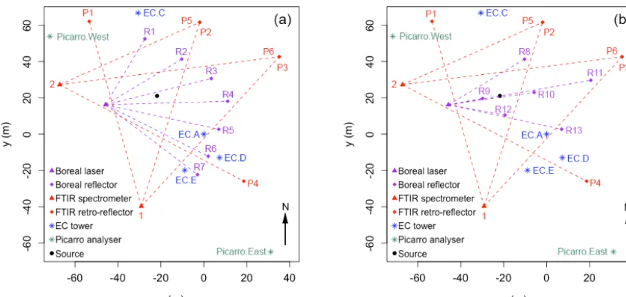
A full description of the experimental setup, measurement techniques, and quantification methods used in the 2015 Gin-ninderra release experiment are given in Feitz et al. (2018). Briefly, CH4(together with CO2and nitrous oxide) was re-leased from a small chamber located in a fallow agricul-tural field from 23 April to 12 June 2015 and from 23 to 24 June 2015. A variety of CH4sensors were placed around the release chamber. The measurement data considered in this study were obtained from two Picarro G2201-i analysers (positioned in the predominant upwind (NW) and downwind (SE) location of the release chamber, labelled Picarro.West and Picarro.East, respectively), four eddy covariance (EC) towers equipped with Li-COR 7700 open-path CH4 sen-sors (labelled EC.A, EC.C, EC.D, and EC.E, respectively), two scanning Fourier-transform infrared (FTIR) spectrome-ters with four retro-reflectors terminating six measurement paths (labelled P1 to P6, respectively), and a scanning Gas-Finder 2 Boreal laser with seven reflectors forming seven measurement paths (labelled R1 to R7, respectively); see the left panel of Fig. 1. Meteorological data were collected from
EC.A equipped with a Vaisala HMP50 relative humidity and temperature sensor, a CSI EC150 CO2–H2O sensor, a Li-COR 7700 CH4sensor, a Kipp and Zonen CNR4 radiome-ter, a CSI CSAT3 sonic anemomeradiome-ter, and a Gill WindSonic anemometer. Wind speed and wind direction were measured by the CSAT3 sonic anemometer and the Gill WindSonic anemometer. As part of data quality control, horizontal wind speed and wind direction data from the two instruments were compared, with no arising issues. Both sonic anemometers were using factory calibration. Wind directions were deter-mined by manually aligning the sonic anemometers so that the reference direction was true north. Data from CSAT3 sonic anemometer were logged at 10 Hz and data from the Gill WindSonic anemometer at 1 Hz.
The gases were released at a height of 0.3 m, and the stan-dard CH4release rate was 5.8 g min−1, limited mostly to day-light hours. On brief occasions, the CH4release rate was var-ied between 2.9 and 20 g min−1 to enable testing of mobile CH4 sensor platforms. Towards the end of the experiment (8–12 June), the CH4release rate was decreased from 5.8 to 5.0 g min−1, and the setup for the Boreal laser measurements was modified with the number of retro-reflectors and paths reduced to six (labelled R8 to R13, respectively; see the right panel of Fig. 1). The location of all other CH4sensors did not change over the duration of the experiment. The Picarro anal-ysers were not deployed until 21 May, and the CH4 release rate on 23 and 24 June was constantly varied. Hence, in this article we only consider data between 21 May and 12 June, excluding 26 and 27 May where the release rate was also constantly varied.
The data set used to obtain the results presented in Sect. 5 was compiled by pooling together the separate meteorologi-cal and concentration data sets used in the Ginninderra exper-iment. A common resolution of 5 min was chosen; that is, all measurements of concentration and meteorological variables were averaged over a regular set of 5 min intervals. Measured CH4 concentrations were then matched with corresponding meteorological measurements by time and placed into long-table format, with each row corresponding to a unique data point. For path measurements, two extra columns were used to denote the end-point coordinates of the paths.
Figure 1. (a)Layout of instruments in the 2015 Ginninderra release experiment between 21 May and 7 June 2015.(b)Layout of instruments between 8 and 12 June 2015. R1 to R13 are the paths formed between the Boreal laser and reflectors; P1 to P6 are the paths formed between the FTIR spectrometers and retro-reflectors; EC.A to EC.E are the EC towers; and Picarro.East and Picarro.West are the Picarro analysers. All coordinates are relative to EC.A, which is situated at the origin.
3 Transport modelling
In this section we detail the plume model employed and how it is used to supply model-predicted concentrations for the path measurements.
3.1 Gaussian plume dispersion modelling
As outlined in Sect. 1, we use a transport model that is sim-ply parameterised, and easy to evaluate, so that it can be cali-brated online. One of the simplest models that works well on the short distances we consider is the Gaussian plume dis-persion model (e.g. Wark et al., 1998, chap. 4). Here the true emission rate is denoted byQin grams per second (g s−1), the height of the CH4point source byH in metres (m), and the total number of observations byN. The classic Gaussian plume model is given by
C xi, yi, zi, Q, Ui, H,θki
= Q
2π Uiσyi,kiσzi,ki
exp − y 2
i
2σy2
i,ki !
"
exp −(zi−H ) 2
2σz2
i,ki !
+exp −(zi+H ) 2
2σz2
i,ki !#
, (1)
where C is the model-predicted concentration in grams per cubic metre (g m−3) of CH4 at a single spatial point
(xi, yi, zi)in metres (m) along the direction of the plume
corresponding to theith measurement,Ui is the wind speed
associated with the ith measurement in metres per second (m s−1),ki∈ {A, B, C, D, E, F}represents the Pasquill
sta-bility class (a categorisation reflective of the expected level of horizontal and/or vertical spread of the atmospheric par-ticles after emission; see Pasquill, 1961) associated with the
ith measurement, andθki represents plume-specific
parame-ters used to construct the standard deviationsσzi,kiandσyi,ki.
These standard deviations of the plume in the vertical and horizontal directions are given by
σzi,ki=akix
bki
i ,
σyi,ki=0.4651xitan(νi),
respectively, where νi=0.01745 cki−dkiln(xi/1000)
. Note that the coefficients aki, bki, cki, dki correspond to
the ith measurement and depend on the stability class associated with that measurement, ki∈ {A, B, C, D, E, F}.
Values for these coefficients by stability class are given in Wark et al. (1998, chap. 4) and shown here in Table 1 for completeness. We collect the plume-specific parameters in θki≡(aki, bki, cki, dki)
0, where 0 denotes the transpose
operator.
The stability class to which an observation is allocated is classically based on (i) the Monin–Obukhov length (the theoretical height at which turbulence is produced by buoy-ancy and mechanical forces in equal amounts; see Sienfeld and Pandis, 2006, chap. 16) and (ii) an effective roughness length. The Monin–Obukhov length (L value) is given by
L= −u3∗ξv/(qg(w∗ξ∗
v)s)(Jacobson, 2005, chap. 8), where
u∗is the frictional velocity,ξv is the mean virtual potential
temperature,(w∗ξ∗
v)sis the surface virtual potential
Table 1.Stability classes to which observations within the Ginninderra experiment are allocated, and the corresponding values ofaki, bki, cki,
anddkiused to construct the horizontal(σyi,ki)and vertical(σzi,ki)standard deviations of the plume whenxi is in metres (m).
Stability class (ki) Stability condition aki bki cki dki
A Extremely unstable 0.17993 0.94470 24.167 2.5334 B Moderately unstable 0.14506 0.93198 18.333 1.8096 C Slightly unstable 0.11025 0.91465 12.500 1.0857 D Neutral 0.084739 0.86974 8.3330 0.72382 E Slightly stable 0.075005 0.83660 6.2500 0.54287 F Moderately stable 0.054370 0.81558 4.1667 0.36191
www.thunderbeachscientific.com/windtrax.html, last access: 27 March 2019) to determine theLvalue for each observa-tion; we provide the L values with the compiled data. We set the effective roughness length z0=0.01 m, correspond-ing to a relatively flat area, with short or no grass, and min-imal buildings/trees/other obstacles; see Sienfeld and Pan-dis (2006, chap. 16) and World Meteorological Organisation (2008, chap. 5). This is a suitable choice for the Ginninderra site. We used the results of Golder (1972) to allocate a stabil-ity class to each observation based on theLvalues provided by WindTrax andz0=0.01 m.
The coefficients typically used for each stability class could be off by a factor of 2 or more (Wark et al., 1998, chap. 4). To show that this is also the case with our categori-sation scheme, in Fig. 2 we show the Gaussian-plume-model-predicted outputs together with the observed data enhance-ments (see Sect. 4.1) at one of our measurement locations (namely, EC.A) between 21 May and 7 June, when scaling
σyi,ki by 1, 2.5, and 4, respectively. Clearly, with no scaling
the predicted plume is too narrow, while with a scaling of 4 it is too broad. A scaling of 2.5 gives good agreement. Impor-tantly, since in Eq. (1)Qonly serves to scale the predicted concentrations (i.e. make them larger or smaller by a con-stant factor), it is apparent that this plume-scaling factor is identifiable, in the sense that we can learn it from the data while estimating the emission rate (provided the source is active). Online plume-model calibration fits naturally within the MCMC framework discussed in Sect. 4.
3.2 Low wind speeds
It is well known that the Gaussian plume model is less ac-curate for low wind speeds (e.g. Turner, 1994, chap. 2). One reason for this is that the wind speedUi is in the
denomi-nator of the scaling coefficient of Eq. (1); hence, the plume model prediction becomes very sensitive to Ui as it tends
towards zero. This is problematic asUi, although often
as-sumed known, is an average calculated from noisy measure-ments taken over some time span (in our case 5 min) and is thus itself noisy. From Eq. (1) we see that, when conditioned on all other parameters, the variance ofCiis proportional to
the variance of the inverse of Ui, which can be very large
for smallUi. Instead of removing data at low wind speeds as
is often done (e.g. Feitz et al., 2018), we analyse the theo-retical relationship between the variance of the inverse wind speed andCi. We then use this relationship to discount
low-wind-speed model predictions in the Bayesian framework in a principled manner. While the analyst still needs to choose a cutoff below which to model this relationship, in separate studies we found that our inferences are not particularly sen-sitive to the chosen cutoff. Moreover, we found that down-weighting instead of excluding was necessary for making inference when not many observations associated with high wind speeds were available.
Each wind speedUi is an average of a number of wind
speeds (saynUi) recorded over 5 min. ThereforeUiis a
sam-ple mean and thus an unbiased estimator of the true (popula-tion) mean wind speed, sayµUi, over this time interval. By
the central limit theorem,√nUi(Ui−µUi)
D
−→Gau(0, σU2
i),
whereDimplies convergence in distribution, Gau(µ, σ2) de-notes the Gaussian distribution with meanµ and variance
σ2, andσU2
i is the variance of the wind speeds over theith
time interval, which was derived from the raw (disaggre-gated) data. We can then use the delta method (e.g. Casella and Berger, 2002, chap. 5) to deduce that
√
nUi
1
Ui
− 1
µUi
D
−→Gau 0,
d
dµUi
1
µUi
2
σU2
i !
.
Hence, the variance of 1/Uiis approximately
d
dµUi
1
µUi
2
σU2
i=
1
µ4U
i
σU2
i∝
1
µ4U
i
.
Therefore, conditional on all other terms in Eq. (1), the variance of the model-predicted concentrations increases as a quartic of the true inverse wind speed. This is important, as it means that model predictions at low wind speeds, say less than 1 m s−1, could be highly uncertain; we show a way of handling this uncertainty when we detail the Bayesian inver-sion model in Sect. 4.
3.3 Predicted concentrations for point and path measurements
plume-Figure 2.Predicted (blue) and observed (red) enhancements in parts per million (ppm) at EC.A between 21 May and 7 June 2015 when scalingσyi,kiby 1, 2.5, and 4, respectively. The mean-squared errors (MSE) between the observed and the predicted enhancements are also
shown. Of the three, the best agreement between predicted and observed values occurs whenσyi,kiis scaled by 2.5.
model concentration at a physical location(exi,eyi,ezi)is thus found by first applying a spatial shift and time-dependent ro-tation (by wind direction) to (exi,eyi,ezi)in order to obtain
(xi, yi, zi), which is then used to compute a model-predicted
concentration (conditional onQ,Ui,H, andθki). Conversion
to parts per million (ppm) is done via the ideal gas law. Let Ci be a model-predicted concentration
(i=1,2, . . ., N). IfCi corresponds to a point measurement,
then one needs only to evaluate Eq. (1) at the transformed point-measurement location to obtain a predicted concen-tration. IfCi corresponds to a path measurement, however,
it represents an average of concentrations along the path. Denote the transformed end points of the straight-line path in the horizontal plane as(xi,1, yi,1)and(xi,2, yi,2), respec-tively. The line between the given points in the horizontal plane can be parameterised by ρi(s)=(ρx,i(s), ρy,i(s))0,
where
ρx,i(s)=sxi,2+(1−s)xi,1, s∈ [0,1],
ρy,i(s)=syi,2+(1−s)yi,1, s∈ [0,1],
so that
Ci =
1
Ti
1 Z
0
C ρx,i(s), ρy,i(s), zi, Q, Ui, H,θki
dρi(s)
ds
ds, (2)
where Ti∈R+ is the path length and k · kis the standard
Euclidean norm. In our case,Ti=
dρi(s)
ds
is not a function ofs, and so Eq. (2) simplifies to
Ci=
1 Z
0
C(ρx,i(s), ρy,i(s), zi, Q, Ui, H,θki)ds.
This integral can be approximated numerically over a fine partitioning of J segments P = {[s0, s1],[s1, s2], . . .,[sJ−1, sJ]}, where 0=s0< s1<
. . . < sJ−1< sJ =1. Then
Ci≈ J
X
j=1
C(ρx,i(sj∗), ρy,i(sj∗), zi, Q, Ui, H,θki)1s,
where1s≡sj−sj−1=1/J andsj∗=
sj+sj−1
2 . In our exper-iments we setJ=100.
4 Bayesian atmospheric tomography
We are ultimately interested in obtaining a range of plausi-ble values for the emission rate,Q, a posteriori, (i.e. after we have observed some data). In this section we present a hierarchical statistical model that relatesQto the observed concentrations via the Gaussian plume model. AlthoughQ
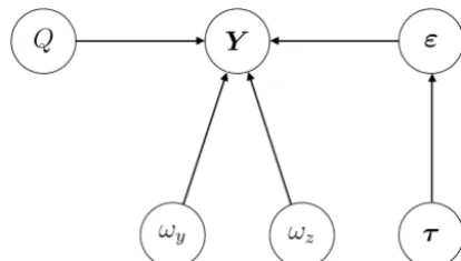
itself is univariate, the model contains several other unknown parameters that capture our uncertainty about the physical and the measurement processes; inferences on these param-eters andQare made simultaneously. For ease of exposition we adopt the terminology of Berliner (1996) to describe the model, which we also summarise graphically in Fig. 3. The top layer in the hierarchy is the data model (the model for the observations,Y, Sect. 4.1), the middle layer is the process model (the model forQ, Sect. 4.2), and the bottom layer is the parameter model (the unknown parameters not of di-rect interest,τ,ωy, ωz, Sect. 4.3). In Sect. 4.4 we outline the
MCMC strategy we use to make inference with the model.
4.1 The data model
Let eY≡(Ye1,eY2, . . .,YeN)0 denote the measured
Figure 3.Directed acyclic graph showing the conditional depen-dence relationships between the data (enhancements)Yand the er-ror componentsε(Sect. 4.1); the emission rateQ(Sect. 4.2); and the unknown parametersτ, ωy,andωz(Sect. 4.3).
ith Gaussian-plume-predicted concentration,Xi is the sum
of the ith CH4 background concentration and instrument-specific bias, and εi denotes the random error associated
with the ith observed CH4 concentration. The background concentration and bias can be explicitly modelled and pre-dicted (Ganesan et al., 2015). Here, as in Zammit-Mangion et al. (2015), we estimateXi as the 5th percentile of all the
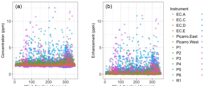
measurements from the instrument associated with the ith measurement. Figure 4 compares the raw averaged concen-trations to those corrected for background and instrument-specific bias, which we term enhancements, when plotted against wind direction (in degrees east of north).
Now, letY≡(Y1, Y2, . . ., YN)0 denote the enhancements,
andε≡(ε1, ε2, . . ., εN). It is straightforward to verify that
Yi=eYi−Xi
=Ci+εi, i=1, . . ., N.
Therefore,Yiis made up of two main components of
variabil-ity: the Gaussian-plume-predicted concentration and a ran-dom error term. We assume that the εi terms are Gaussian
and independent but that they are not identically distributed. Specifically, εi contains two components of variation, one
pertaining to the error characteristics of the instrument and one to the stability class with which we have categorised the measurement. Recall also from Sect. 3.2 that we model the variance of the predicted concentrations to be propor-tional to a quartic of the true mean inverse wind speed for
Ui<1 m s−1.
First, we capture instrument-specific measurement er-ror characteristics and stability-condition-specific variation by introducing an auxiliary variable mi (mi=1,2, . . ., M),
whereMis the total number of unique combinations of sta-bility class and instrument type, and consider M different precision (i.e. inverse variance) parameters {τmi}that need
to be estimated, one for each combination. Second, we take the influence of low wind speeds into account by assuming that the precision of εi isτmi multiplied byUˆi, where, for
Ui >0,
ˆ
Ui =
(
Ui4 0< Ui<1,
1 Ui≥1,
(3)
which encapsulates our prior belief that observed model– measurement mismatch variability at low wind speeds (in this case under 1 m s−1) is dominated by the low wind speed. Putting these two components together, we have that, con-ditional on the instrument type and stability class encoded in
mi,
εi |mi∼Gau(0,1/(Uˆiτmi)), i=1, . . ., N.
We detail the prior distribution forτmiin Sect. 4.3.1.
4.2 The process model
The process of interest in this application is the emission rate,
Q, which we assume is constant. Since in this application
Q≥0, we model it using a half-normal prior distribution (a Gaussian distribution with mean zero truncated from below at zero),
p(Q)=
√
2
σQ √
πexp
−Q2
2σ2 Q
, Q ∈ [0,∞)
0 otherwise,
(4)
with a standard deviation parameter, σQ, which is known
and fixed. In our case we fixedσQto 1.5 g s−1(90 g min−1),
which results in a relatively uninformative prior distribution. While addressing nonnegativity, half-normal priors do not contain a point mass at zero and thus do not encode a prior belief that there is a possibility of having exactly a zero emis-sion rate. As a consequence, a posterior estimate or even a credible interval that includes zero is not possible. A spike-and-slab distribution (Mitchell and Beauchamp, 1998) con-sisting of a diffuse uniform distribution with a point mass at zero could be alternatively used at the cost of a slightly more complex model.
4.3 The parameter model
Our parameter model is divided into two parts: one pertaining to the precision parameters{τmi}in the random-error
com-ponent in the data model; and the other to the standard de-viations in the Gaussian-plume dispersion models which, as shown in Sect. 3.1, are also uncertain.
4.3.1 The precision parameters
For conjugacy with the Gaussian likelihood, we model each
τmi using a Gamma prior distribution, with shape parameter
αand rate parameterβ:
p(τmi)=
βα 0(α)τ
α−1
mi e
Figure 4. (a)Raw averaged concentrations, plotted by instrument and against wind direction.(b)Enhancements obtained by subtracting off the background and instrument-specific bias.
In our application we set α=1.058 andβ=0.621. These values were chosen through quantile matching, such that the 1st and 99th percentiles of the distribution of 1/√τmi are
approximately 0.35 and 6.5 ppm, respectively (giving a mode close to 0.7 ppm). Values for these percentiles were selected based on prior exploratory data analysis of the measurements that were taken upwind of the source.
4.3.2 The Gaussian plume model parameters
From separate studies into the reliability of the model values for σyi,ki andσzi,ki, briefly discussed in Sect. 3.1, we
con-cluded that these parameters could indeed be off by factors of 2 or more and that, if they are off, they are so by simi-lar amounts for each stability class. These factors correspond to vertical shifts of the Pasquill stability curves when plot-ted on a log–log scale (e.g. Wark et al., 1998, chap. 4). We thus replacedσyi,kiandσzi,kiin Eq. (1) witheσyi,kiandeσzi,ki,
respectively, where
eσyi,ki≡ωyσyi,ki
and
eσzi,ki≡ωzσzi,ki,
andωy, ωz∈R+are scaling parameters forσyi,kiandσzi,ki,
respectively (Borysiewicz et al., 2012).
We use Gamma prior distributions forωy andωz. In our
application we set the shape parameters equal to 1.6084 and the rate parameters equal to 0.7361. These parameters give approximate 1st and 99th percentiles of 0.1 and 8, respec-tively, and a mode close to 1 (representative of no scalar in-fluence onσyi,ki orσzi,ki). This reflects our prior belief that
the standard deviations could be up to an order of magnitude off from those derived using classical Pasquill stability-class theory.
4.4 Bayesian inference
Recall Y≡(Y1, Y2, . . ., YN)0 are the N observed
en-hancements, and let U≡(U1, U2, . . ., UN)0 and 2≡
(θk1,θk2, . . .,θkN)
0. Further, let τ≡(τ
1, τ2, . . ., τM)0 be the
M parameters associated with each combination of instru-ment type and stability class. The posterior distribution of the emission rateQis then given by
p(Q|Y,U, H,2)
∝ ∞ Z
0
∞ Z
0 Z
RM+
p(Y,τ, ωy, ωz|Q,U, H,2)p(Q)dτdωydωz
=p(Q)
∞ Z
0
∞ Z
0 Z
RM+
p(Y |Q,τ, ωy, ωz,U, H,2)
p(τ)p(ωy)p(ωz)dτdωydωz,
where p(Q) is given by Eq. (4) and p(Y|
Q,τ, ωy, ωz,U, H,2)is the likelihood, which is Gaussian.
Computation of the posterior distribution p(Q| Y,U, H,2) involves a high-dimensional integral that is analytically intractable. We therefore use MCMC, specifi-cally a Gibbs sampler, to obtain samples from the posterior distributions ofQ,τ, ωy, andωz (see Gelman et al., 2013,
for a comprehensive introduction to MCMC). The Gibbs sampler samples each parameter one at a time from their re-spective full conditional distributions, where conditioning is done using the most recent samples of all other parameters.
distributions, with Gaussian proposals and adaptive scaling during the early stages of the MCMC algorithm. Specifically, for each parameter, the standard deviation of the proposal was increased or decreased as appropriate whenever the ac-ceptance rate fell below 10 % or exceeded 80 %.
5 Results and discussion
5.1 Observing system simulation experiment
In this section we discuss results from applying our model to simulated data in an observing system simulation experiment (OSSE). To mimic the conditions in the real experiment, we simulated enhancements using the actual Boreal and EC instrument locations, meteorological observations from the Ginninderra data, and realistic variances for the random-error components. We considered the two release-rate periods sep-arately, using a 6 g min−1 emission rate in the first and a 12 g min−1emission rate in the second. As in the real exper-iment, the first Boreal laser/reflector setup (seven paths) was used in the first release-rate period, while the second setup (six paths) was used in the second release-rate period; the EC tower locations were kept constant for both periods. We set the precisionsτmi=4 formi=1, . . ., M and the scaling
factorsωy=ωz=2 to assess the algorithm’s ability to
cali-brate the plume online. Following data simulation, we used MCMC to generate 60 000 samples, left out 20 000 of these as burn-in, and used a thinning factor of 10. Adaptation of the Metropolis samplers was only done during burn-in. Conver-gence was assessed through visual inspection of the MCMC trace plots.
We made inference onQ, as well as all other parameters in the model, for the Boreal- and EC-simulated data and the two emission rate settings. Table 2 shows the posterior me-dian emission rates, the 95 % posterior credible intervals for the emission rate, and the intervals for the plume standard deviation scaling parametersωyandωz. In all cases, we see
that the true (simulated) emission rate is captured within our posterior credible intervals and that the median estimates are very close to the true values. Interestingly, we see that while the plume-scaling coefficients have been accurately recov-ered in most cases, the posterior uncertainty overωyfor the
Boreal lasers is very wide. This suggests thatωymight not be
identifiable for path measurements, possibly because the av-eraging effect of the line integral renders the measured con-centration insensitive to a specific plume width in the hori-zontal direction.
5.2 Application to the Ginninderra data set
In this section we discuss results from applying our model to enhancements from the compiled Ginninderra data. We con-sidered several settings. In the first setting, we estimated the emission rate separately for each of the four instrument types and for each release-rate period (5.8 and 5.0 g min−1) when
the source was active. In addition, for each release-rate pe-riod we estimated the emission rate for all the instruments combined, yielding a total of 10 inversion results. In the sec-ond setting we estimated the emission rate for the same 10 cases but for periods when the source was switched off. In the third setting we again considered the same 10 cases but using only measurements that were taken when upwind of the source. These three settings serve to demonstrate how our inferences adapt to the various settings one might encounter in the field. In particular, online plume calibration is almost impossible in the latter two settings, and we expect this to result in large posterior uncertainties on the scaling coeffi-cients, and also the emission rate in the third setting. In the second setting downwind measurements are present. There-fore, while online plume calibration is again almost impos-sible since there is no active source, the absence of a source (Q=0 g min−1) should be reflected in our posterior infer-ences (recall, however, that use of a half-normal prior distri-bution precludes the possibility of a zero emission rate being estimated; see Sect. 4.2).
As in the OSSE, we generated 60 000 MCMC samples, left out 20 000 of these as burn-in, and used a thinning factor of 10. In line with what we observed in the OSSE, our initial results showed that, more often than not,ωy is not
identifi-able (leading to wide posterior distributions and poor MCMC mixing) when attempting to estimate the emission rate with the source switched on with path measurements. We there-fore chose to fixωy=1 (but notωz) for path measurements,
Figure 5. (a) Posterior empirical distributions of the emission rateQ in grams per minute (g min−1), for the Boreal lasers (B), FTIR spectrometers (F), EC towers (E), Picarro analysers (P), and the ensemble of all instruments (BFEP), for each release-rate period (1 and 2) during the Ginninderra experiment. The 5.8 g min−1release-rate period is shown in red (B1, F1, E1, P1, and BFEP1), while the 5.0 g min−1 release-rate period is shown in blue (B2, F2, E2, P2, and BFEP2). The vertical dashed lines denote the respective true emission rates, the black dots denote the median estimates, and the black vertical bars denote the upper and lower limits of the 95 % posterior credible intervals.
(b)Same as(a)but showing results obtained using measurements taken when the methane point source was inactive. In both cases, we can recover a reasonable range of estimates for the emission rate, with no 95 % posterior credible interval being far from the true emission rate. Further, we see that the posterior emission rate credible intervals move towards zero when the source is inactive, as desired.
at a common temporal resolution – no manual instrument-specific tuning was carried out. The approach thus seems rel-atively robust to instrument type; in Sect. 6 we show this is no longer the case once certain components in our model are assumed fixed and known.
The first 10 rows of Table A1 also show the 95 % poste-rior credible intervals forωy andωz.None of the obtained
credible intervals forωy contain 1, and the results
corrob-orate the conclusion from our exploratory data analysis in Sect. 3.1 that a plausible value forωy is about 2 or 3. This
stability-class curves corresponding to σyi,ki while
estimat-ing the emission rate with point measurements. There was less agreement onωzin the inversions, suggesting that
some-thing more complex than a simple scaling is required (or that the model used for σzi,ki is, in this case, inappropriate) for
calibrating the Pasquill stability-class curves corresponding toσzi,ki. Nonetheless, in Sect. 6 we show that our
emission-rate estimates from point measurements were relatively less sensitive to the assumption ωz=1 than to the assumption
ωy=1.
The right panel in Fig. 5 summarises our results for Q
in the second setting (both upwind and downwind measure-ments with the source switched off), while full results are given in the second set of 10 rows in Table A1. Recall from Sect. 4.2 that, due to the choice of prior overQ(a half-normal distribution), it is not possible for the 95 % credible inter-val to include zero. Clearly, however, the interinter-vals forQare close to zero and are suggestive of a small emission rate. As expected, the plume standard deviation scaling parameters are not well-constrained in this setting when the source is off: narrow credible intervals on the emission rate here are only possible when the measurement is largely insensitive to the plume shape. This is indeed the case for the Boreal paths, some of which pass very close to the source. With other in-strument configurations, uncertainty in the plume scalings dominates. In some cases (FTIR spectrometers and Picarro analysers in the 5.0 g min−1release-rate period) our MCMC algorithm did not converge after the 60 000 samples; these results are thus omitted from Fig. 5 and Table A1.
The bottom 10 rows in Table A1 give full results in the third setting (upwind measurements only with the source switched on). In this setting the 95 % posterior credible in-tervals produced for the emission rates are very wide (most with a range of over 100 g min−1), as are those produced for
ωy and ωz: our posterior distributions are largely
uninfor-mative. This was expected since upwind measurements con-tain no information on both the emission rateandthe plume model parameters. These results from upwind measurements serve as verification and confirm that we are indeed relying on useful information from downwind measurements when making inference on the emission rate and other parameters that appear within our model.
6 Sensitivity of results to model components
As detailed throughout Sect. 4, the Bayesian model we employ contains many parameters that are updated using MCMC. A natural question to ask is whether all these pa-rameters do need to be updated and what the effects on the emission rate inferences are when instead some of these are assumed fixed and known. Specifically, we are interested in seeing what happens when (i) considering only one single precision parameterτ for all of the data regardless of stabil-ity class and/or instrument group, (ii) considering oneτmiper
instrument group only, (iii) not accounting for plume-model variability in low wind speeds (i.e. settingUˆ =1), (iv) not updatingωywhen using point measurements, (v) not
updat-ingωz, and (vi) not updating both ωy andωz when using
point measurements. The 95 % credible intervals for Qin grams per minute for all these settings and for each of the 10 groupings considered in Sect. 5 are given in Table A2.
Grouping the precision parameters {τmi} by instrument
only (instead of by instrument and stability class) had a slightly negative impact on the emission-rate estimates ob-tained during the second release-rate period but less so during the first release-rate period. Assuming (and fixing)ωz=1 for
both the point and path measurements also did not have a se-rious impact on the emission-rate estimates. Note that this does not mean that these components are not relevant in the general model – for example, from our estimates ofωzin
Ta-ble A1 we seeωz=1 would be a plausible choice for this
experiment if one opted to fixωz (whileωy=1 would not
be).
On the other hand several components in our model appear to be crucial to obtaining reasonable emission-rate estimates. Using a single precision parameter to capture all observed variability due to measurement error and the stability-class categorisation clearly had a negative impact on our emission-rate estimates. Similarly, assuming the variability of the mea-surements is independent of wind speed when performing in-version resulted in 95 % posterior credible intervals on the emission rate that are considerably shifted in the negative direction. A similar observation was made by Feitz et al. (2018, p. 207) when analysing data from the Boreal lasers. There, observations with wind speeds below 1.5 m s−1were removed to mitigate this effect.
The scaling factor ωy is clearly also crucial for
obtain-ing emission-rate estimates of practical significance for point measurements, with the ensuing emission-rate estimates of-ten being off by nearly a factor of 2 whenωy=1 is assumed.
As expected, the width of the credible intervals on the emis-sion rate decreased substantially whenωy=ωz=1 was
as-sumed, indicating thatωy andωz play a big role in
quanti-fying uncertainty on the emission rate. Therefore, as noted in other studies discussed in Sect. 1, incorporating uncer-tainty in the transport model by treating parameters within the model itself as uncertain (note that this is different from adding another component of variability in the data model, as is often done) is likely to have a positive impact on emission-rate estimates and uncertainty quantification.
7 Conclusions
dif-bling from a creek or where measurement is hazardous. De-pending on the circumstance, detection of leakage can take many different forms, from visible bubble detection, optical gas imaging, handheld sniffers, noise detection, helicopters equipped with lasers, drones equipped with gas sensors, to monitoring die-off in vegetation using remote sensing tech-niques. Surface leakage typically expresses as small, concen-trated hotspots if sourced from the subsurface (Feitz et al., 2014; Forde et al., 2019), for which the quantification ap-proach outlined in this article is ideally suited. Equipment placement can be optimised around the leakage site (i.e. pre-vailing upwind/downwind) for optimal quantification.
In most applications neither the number of sources nor the source location is known. As such, the framework we con-struct should be seen as a foundational building block that needs to be extended appropriately for each specific applica-tion. For example, if the source location is not known, then source localisation can be incorporated into the Bayesian framework as discussed by Humphries et al. (2012). If there are multiple possible sites, and these locations are not known, then the framework needs to be further extended to incorpo-rate multiple Gaussian plume models (one for each site), and joint localisation–inversion will be required. While these ex-tensions are straightforward both mathematically and com-putationally, in practice they are unlikely to be effective for detection of leakage over large spatial scales. Gas fields or geological storage sites can cover areas of tens to hundreds of square kilometres. Unless there is a high density of sen-sors (≈100 m scale, van Leeuwen et al., 2013; Jenkins et al., 2016), the sensitivity of detection will be poor (Wilson et al., 2014; Luhar et al., 2014). It is however relatively straight-forward to effectively extend the methodology to when the emission is from an area rather than a point source.
Our work is closely connected to other atmospheric to-mography techniques but with some small, significant, differ-ences. Luhar et al. (2014) used a backward Lagrangian parti-cle model to simulate the trajectories of methane and carbon dioxide backwards in time to localise the source and estimate the emission rates. Their approach yielded good quality es-timates for the methane emission rates but highly uncertain estimates for the carbon dioxide emission rates and source location parameters. Twenty-three runs of the Lagrangian
to that of Humphries et al. (2012); we see from our results that having this hard constraint is not a tenable assumption in practice. Our work also has close connections with that of Ars et al. (2017) where the Pasquill stability class for an observation is chosen from a subset of appropriate stability classes, based on the best fit of model-predicted values to observed values. While this may help fit the Gaussian plume dispersion model to the data, it does not take into account the uncertainty arising from stability-class choice. Further, if all plume model standard deviations are off by a factor of 2 or more, there is a distinct possibility that no stability class yields a good fit. Online calibration of these standard devi-ations is needed to account for lack-of-fit arising from the inherently simple Gaussian plume model.
much lower for the more neutral stability classes C and D than for the more stable/unstable classes A and F.
The fully Bayesian framework we adopt is adaptable to various scenarios. We envision, for example, that source lo-calisation (e.g. Humphries et al., 2012; Hirst et al., 2013) could be done in tandem with plume-model calibration within an inversion framework, provided several instruments in suitable configurations (as in the Ginninderra experiment) are available. Future work will also investigate how un-certainty in other meteorological variables such as wind-direction, as well as the stability-class categorisation adopted (possibly viaz0), could be incorporated within the model.
Source on BFEP1 5.9008 (5.7050,6.1038) (2.3360,2.5640) (1.1944,1.2989) (upwind and downwind) B2 5.1552 (4.2571,6.1820) – (0.84608,1.1288) F2 4.0525 (3.2838,4.8497) – (0.66723,1.0944) E2 4.2017 (3.6297,4.8923) (1.4899,2.1671) (0.90941,1.0981) P2 3.2135 (2.1071,4.7236) (2.0250,5.2798) (0.34677,0.63648) BFEP2 3.9455 (3.5054,4.4543) (1.7138,2.5325) (0.97964,1.1437)
B1 0.52073 (0.40106,0.71608) – (1.3051,5.0262) F1 0.72641 (0.36438,1.5935) – (1.2565,9.0531) E1 1.6906 (0.95997,3.2742) (10.768,21.971) (3.1036,11.826) P1 1.7798 (0.61237,5.6367) (3.3985,13.853) (0.31311,7.3589) Source off BFEP1 0.65416 (0.52512,0.87510) (7.0545,12.789) (2.2381,5.3166) (upwind and downwind) B2 0.52202 (0.31479,0.77494) – (0.84995,1.5319)
F2 n/a n/a – n/a
E2 0.85549 (0.32681,3.3683) (2.3136,11.371) (0.50337,7.9746)
P2 n/a n/a n/a n/a
BFEP2 0.72846 (0.34557,1.5735) (2.7823,9.5185) (0.97971,7.1704)
Table A2.Posterior 95 % credible intervals for the emission rates in grams per minute (g min−1) for the Boreal lasers (B), FTIR spectrometers (F), EC towers (E), Picarro analysers (P), and an ensemble of all instruments (BFEP), for each release-rate period (5.8 g min−1(1), and 5.0 g min−1(2)) and for various alterations to the model as detailed in Sect. 6. Dashes correspond to the redundant case (e.g.ωy=1 was
assumed for all path measurements in the full model).
Full model Assuming Assuming
Group formi= τmi=τinstrument {τmi}are only Assuming
1, . . ., M group dependent Uˆ =1
B1 (5.4733,6.5593) – (4.7238,5.6727) (2.6092,3.1975) F1 (6.1985,7.2937) – (5.9526,7.1190) (3.6482,4.7116) E1 (6.2942,6.9537) – (6.2062,7.0047) (5.4894,5.9759) P1 (4.2710,5.6136) – (4.8748,6.1139) (2.9868,3.9053) BFEP1 (5.7050,6.1038) (4.7252,5.2433) (5.8133,6.2731) (3.4032,3.6424) B2 (4.2571,6.1820) – (4.0863,6.4436) (2.5337,3.5319) F2 (3.2838,4.8497) – (2.7180,4.2555) (1.4055,2.1349) E2 (3.6297,4.8923) – (3.2692,9.4560) (3.1329,4.1516) P2 (2.1071,4.7236) – (1.6784,4.7147) (1.8451,3.0813) BFEP2 (3.5054,4.4543) (2.5283,3.4837) (2.3224,3.2790) (1.9421,2.4779)
Group Assuming Assuming Assuming
ωy=1 ωz=1 ωy=ωz=1
B1 – (4.0341,4.7974) –
F1 – (5.4152,6.3851) –
E1 (3.3635,3.7084) (6.8646,7.5289) (3.6129,3.8937) P1 (2.0142,2.5424) (5.8880,7.5225) (2.6043,3.4691) BFEP1 (3.6176,3.8644) (5.9888,6.3946) (3.8251,4.0726)
B2 – (4.3543,5.7021) –
F2 – (3.2608,4.7770) –
“The 10th International Carbon Dioxide Conference (ICDC10) and the 19th WMO/IAEA Meeting on Carbon Dioxide, other Green-house Gases and Related Measurement Techniques (GGMT-2017) (AMT/ACP/BG/CP/ESD inter-journal SI)”. It is a result of the 10th International Carbon Dioxide Conference, Interlaken, Switzerland, 21–25 August 2017.
Acknowledgements. Laura Cartwright acknowledges the support of the Australian Government Research Training Program Schol-arship. Laura Cartwright, Andrew Zammit-Mangion, and An-drew Feit would like to acknowledge APR.Intern for facilitating the first 5 months of this modelling study. All authors thank Gareth Davies for reviewing an earlier version of the manuscript. The Gin-ninderra field site was supported by the Australian Government through the Carbon Capture and Storage – Implementation bud-get measure. The authors also acknowledge funding for the re-search provided by the Australian Government through the CRC programme and support from the CO2CRC. The National Geose-questration Laboratory is thanked for making the two Picarro instru-ments available for the study. We would like to thank Phil Dunbar and his staff (CSIRO Plant Industry) for maintaining the site and Dale Hughes (CSIRO) for his assistance with maintenance of the CSIRO EC tower. The authors also wish to acknowledge the assis-tance of Field Engineering Services at Geoscience Australia. Geo-science Australia and the Western Sydney University team would like to acknowledge Charles Jenkins (CSIRO) for early discussions about the atmospheric tomography line technique and the Aus-tralian Mathematical Sciences Institute. The University of Wollon-gong wishes to acknowledge Joel Wilson, Maximilien Desservettaz, and Ruhi Humphries for their assistance in the site operations. An-drew Feitz and Ivan Schroder publish with the permission of the CEO of Geoscience Australia.
Financial support. This research has been supported by the Australian Research Council (grant nos. DE180100203 and FT180100327).
Review statement. This paper was edited by Hubertus Fischer and reviewed by two anonymous referees.
imum Entropy and Bayesian Methods, edited by: Hanson, K. M. and Silver, R. N., Springer, New York, NY, 15–22, 1996. Borysiewicz, M., Wawrzynczak, A., and Kopka, P.: Stochastic
al-gorithm for estimation of the model’s unknown parameters via Bayesian inference, Proceedings of the Federated Conference on Computer Science and Information Systems, Wroclaw, Poland, 501–508, 2012.
Casella, G. and Berger, R. L.: Statistical Inference, 2nd edn., Duxbury Press, Pacific Grove, CA, 2002.
Cartwright, L.: Bayesian atmospheric tomography with application to data from the 2015 Ginninderra release experiment, available at: https://github.com/Lcartwright94/BayesianAT, last access: 1 August 2019.
Chevallier, F., Feng, L., Bösch, H., I. Palmer, P., and Rayner, P.: On the impact of transport model errors for the estimation of CO2 surface fluxes from GOSAT observations, Geophys. Res. Lett., 37, L21803, https://doi.org/10.1029/2010GL044652, 2010. Etheridge, D., Luhar, A., Loh, Z., Leunning, R., Spencer, D. Steele,
P., Zegelin, S., Allison, C., Krummel, P., Leist, M., and van der Schoot, M.: Atmospheric monitoring of the CO2CRC Otway Project and lessons for large scale CO2storage projects, Energy Proceedia, 4, 3666–3675, 2011.
Feitz, A., Leamon, G., Jenkins, C., Jones, D. G., Moreira, A., Bres-san, L., Melo, C., Dobeck, L. M., Repasky, K., and Spangler, L. H.: Looking for leakage or monitoring for public assurance?, Energy Proceedia, 63, 3881–3890, 2014.
Feitz, A., Schroder, I., Phillips, F., Coates, T., Negandhi, K., Day, S., Luhar, A., Bhatia, S., Edwards, G., Hrabar, S., Hernandez, E., Wood, B., Naylor, T., Kennedy, M., Hamilton, M., Hatch, M., Malos, J., Kochanek, M., Reid, P., Wilson, J., Deutscher, N., Zegelin, S., Vincent, R., White, S., Ong, C., George, S., Maas, P., Towner, S., and Griffith, D.: The Ginninderra CH4and CO2 release experiment: an evaluation of gas detection and quantifi-cation techniques, Int. J. Greenh. Gas Con., 70, 202–224, 2018. Flesch, T. K., Wilson, J. D., Harper, L. A., Crenna, B. P., and Sharpe,
R. R.: Deducing ground-to-air emissions from observed trace gas concentrations: A field trial, J. Appl. Meteorol., 43, 487–502, 2004.
Forde, O. N., Mayer, K. U., and Hunkeler, D.: Identification, spatial extent and distribution of fugitive gas migration on the well pad scale, Sci. Total Environ., 652, 356–366, 2019.
hierarchi-cal Bayesian methods, Atmos. Chem. Phys., 14, 3855–3864, https://doi.org/10.5194/acp-14-3855-2014, 2014.
Ganesan, A. L., Manning, A. J., Grant, A., Young, D., Oram, D. E., Sturges, W. T., Moncrieff, J. B., and O’Doherty, S.: Quantifying methane and nitrous oxide emissions from the UK and Ireland using a national-scale monitoring network, Atmos. Chem. Phys., 15, 6393–6406, https://doi.org/10.5194/acp-15-6393-2015, 2015.
Gelman, A., Stern, H. S., Carlin, J. B., Dunson, D. B., Vehtari, A., and Rubin, D. B.: Bayesian Data Analysis, 3rd edn., Chapman & Hall/CRC Press, Boca Raton, FL, 2013.
Golder, D.: Relations among stability parameters in the surface layer, Bound.-Lay. Meteorol., 3, 47–58, 1972.
Harvey, N. J., Huntley, N., Dacre, H. F., Goldstein, M., Thom-son, D., and Webster, H.: Multi-level emulation of a volcanic ash transport and dispersion model to quantify sensitivity to un-certain parameters, Nat. Hazards Earth Syst. Sci., 18, 41–63, https://doi.org/10.5194/nhess-18-41-2018, 2018.
Hirst, B., Jonathan, P., del Cueto, F. G., Randell, D., and Kosut, O.: Locating and quantifying gas emission sources using re-motely obtained concentration data, Atmos. Environ., 74, 141– 158, 2013.
Houweling, S., Bergamaschi, P., Chevallier, F., Heimann, M., Kaminski, T., Krol, M., Michalak, A. M., and Patra, P.: Global inverse modeling of CH4 sources and sinks: an overview of methods, Atmos. Chem. Phys., 17, 235–256, https://doi.org/10.5194/acp-17-235-2017, 2017.
Humphries, R., Jenkins, C., Leuning, R., Zegelin, S., Griffith, D., Caldow, C., Berko, H., and Feitz, A.: Atmospheric tomography: a Bayesian inversion technique for determining the rate and lo-cation of fugitive emissions, Environ. Sci. Technol., 46, 1739– 1746, 2012.
International Energy Agency: Energy Technology Perspectives 2017, OECD/IEA, Paris, France, 2017.
Jacobson, M. Z.: Fundamentals of Atmospheric Modeling, 2nd edn., Cambridge University Press, New York, NY, 2005. Jenkins, C., Kuske, T., and Zegelin, S.: Simple and effective
atmo-spheric monitoring for CO2leakage, Int. J. Greenh. Gas Con., 46, 158–174, 2016.
Jenkins, J. D., Luke, M., and Thernstrom, S.: Getting to zero car-bon emissions in the electric power sector, Joule, 2, 2487–2510, 2018.
Jones, M., Goldstein, M., Jonathan, P., and Randell, D.: Bayes linear analysis for Bayesian optimal experimental design, J. Stat. Plan. Infer., 171, 115–129, 2016.
Kinnon, M. A. M., Brouwer, J., and Samuelsen, S.: The role of nat-ural gas and its infrastructure in mitigating greenhouse gas emis-sions, improving regional air quality, and renewable resource in-tegration, Prog. Energ. Combust., 64, 62–92, 2018.
Lewicki, J. L. and Hilley, G. E.: Eddy covariance mapping and quantification of surface CO2 leakage fluxes, Geophys. Res. Lett., 36, L21802, https://doi.org/10.1029/2009GL040775, 2009. Loh, Z. M., Leuning, R., Zegelin, S. J., Etheridge, D. M., Bai, M., Naylor, T., and Griffith, D.: Testing Lagrangian atmospheric dis-persion modelling to monitor CO2and CH4leakage from geose-questration, Atmos. Environ., 43, 2602–2611, 2009.
Lucas, D. D., Simpson, M., Cameron-Smith, P., and Baskett, R. L.: Bayesian inverse modeling of the atmospheric trans-port and emissions of a controlled tracer release from a
nu-clear power plant, Atmos. Chem. Phys., 17, 13521–13543, https://doi.org/10.5194/acp-17-13521-2017, 2017.
Luhar, A. K., Etheridge, D. M., Leuning, R., Loh, Z. M., Jenk-ins, C. R., and Yee, E.: Locating and quantifying greenhouse gas emissions at a geological CO2 storage site using atmo-spheric modeling and measurements, J. Geophys. Res.-Atmos., 119, 10959–10979, 2014.
Miller, S. M., Hayek, M. N., Andrews, A. E., Fung, I., and Liu, J.: Biases in atmospheric CO2estimates from correlated mete-orology modeling errors, Atmos. Chem. Phys., 15, 2903–2914, https://doi.org/10.5194/acp-15-2903-2015, 2015.
Mitchell, T. J. and Beauchamp, J. J.: Bayesian variable selection in linear regression, J. Am. Stat. Assoc., 83, 1023–1032, 1998. Pasquill, F.: The estimation of the dispersion of wind-borne
mate-rial, Meteorol. Mag., 90, 33–49, 1961.
Peylin, P., Baker, D., Sarmiento, J., Ciais, P., and Bousquet, P.: Influ-ence of transport uncertainty on annual mean and seasonal inver-sions of atmospheric CO2data, J. Geophys. Res.-Atmos., 107, 4385, https://doi.org/10.1029/2001JD000857, 2002.
Rajaona, H., Septier, F., Armand, P., Delignon, Y., Olry, C., Al-bergel, A., and Moussafir, J.: An adaptive Bayesian inference al-gorithm to estimate the parameters of a hazardous atmospheric release, Atmos. Environ., 122, 748–762, 2015.
Riddick, S. N., Connors, S., Robinson, A. D., Manning, A. J., Jones, P. S. D., Lowry, D., Nisbet, E., Skelton, R. L., Allen, G., Pitt, J., and Harris, N. R. P.: Estimating the size of a methane emis-sion point source at different scales: from local to landscape, At-mos. Chem. Phys., 17, 7839–7851, https://doi.org/10.5194/acp-17-7839-2017, 2017.
Sepulveda, N. A., Jenkins, J. D., de Sisternes, F. J., and Lester, R. K.: The role of firm low-carbon electricity resources in deep decarbonisation of power generation, Joule, 2, 2403–2420, 2018. Sienfeld, J. H. and Pandis, S. N.: Atmospheric Chemistry and Physics: From Air Pollution to Climate Change, 2nd edn., John Wiley & Sons, Hoboken, NJ, 2006.
Tarantola, A.: Inverse Problem Theory and Methods for Model Parameter Estimation, SIAM, Philadelphia, PA, https://doi.org/10.1137/1.9780898717921, 2005.
Turner, B.: Workbook of Atmospheric Dispersion Estimates, 2nd edn., Lewis Publishers, Boca Raton, FL, 1994.
van Leeuwen, C., Hensen, A., and Meijer, H. A. J.: Leak detection of CO2pipelines with simple atmospheric CO2sensors for car-bon capture and storage, Int. J. Greenh. Gas Con., 19, 420–431, 2013.
Wang, Y., Huang, H., Huang, L., and Ristic, B.: Evaluation of Bayesian source estimation methods: A comparison of likelihood functions and distance measures, Atmos. Environ., 152, 519– 530, 2017.
Wark, K., Warner, C. F., and Davis, W. T.: Air Pollution: Its Origin and Control, Addison Wesley Longman, Menlo Park, CA, 1998. White, E. D., Rigby, M., Lunt, M. F., Smallman, T. L., Comyn-Platt, E., Manning, A. J., Ganesan, A. L., O’Doherty, S., Stavert, A. R., Stanley, K., Williams, M., Levy, P., Ramonet, M., Forster, G. L., Manning, A. C., and Palmer, P. I.: Quantifying the UK’s carbon dioxide flux: an atmospheric inverse modelling approach using a regional measurement network, Atmos. Chem. Phys., 19, 4345– 4365, https://doi.org/10.5194/acp-19-4345-2019, 2019. Wilson, P., Feitz, A., Jenkins, C., Berko, H., Loh, Z., Luhar, A.,