Evaluation of the Effect of Radius of Curvature on the Rounded Edge Diffraction Loss Computed by Hacking Method for a Plateau

http://www.sciencepublishinggroup.com/j/ajsea doi: 10.11648/j.ajsea.20170602.17

ISSN: 2327-2473 (Print); ISSN: 2327-249X (Online)

Evaluation of the Effect of Radius of Curvature on the

Rounded Edge Diffraction Loss Computed by Hacking

Method for a Plateau

Swinton C. Nwokonko, Ikechukwu H. Ezeh, Vital K. Onwuzuruike

Department of Electrical Engineering, Imo State University (IMSU), Owerri, Nigeria

Email address:

[email protected] (I. H. Ezeh)

To cite this article:

Swinton C. Nwokonko, Ikechukwu H. Ezeh, Vital K. Onwuzuruike. Evaluation of the Effect of Radius of Curvature on the Rounded Edge Diffraction Loss Computed by Hacking Method for a Plateau. American Journal of Software Engineering and Applications.

Vol. 6, No. 2, 2017, pp. 49-55. doi: 10.11648/j.ajsea.20170602.17

Received: January 8, 2017; Accepted: January 18, 2017; Published: June 12, 2017

Abstract:

In this paper, the effect of the radius of curvature on the diffraction loss of rounded edge obstruction is presented. The study is conducted for C-band microwave link with a plateau in its path. The plateau has flat to that spans about 1922 m. Two different approaches are used to determine the radius of curvature of the rounded edged fitted to the plateau top. Among the two methods employed, the ITU-R 526-13 method overestimated the radius (about 12,374,693.37 m) as against 59,031.42 m estimated by the second method at the same C-band frequency of 4 GHz. Also, high radius of curvature by the ITU-R 526-13 method gave very high diffraction loss value for the plateau. Furthermore, with the ITU-R 526-13 method, the radius of curvature does increase with increase in frequency. In all, the results indicate that the ITU-R 526-13 method is not particularly suitable for estimating the radius of curvature for the rounded edge when applied to a plateau. In addition, a more accurate method is required to estimate the radius of curvature for computing rounded edge diffraction loss.

Keywords:

Rounded Edge Diffraction, Diffraction Loss, Elevation Profile, Diffraction Parameter, Knife Edge Diffraction, Hacking Rounded Edge Diffraction Method

1. Introduction

Most obstacle encountered real world cannot be well modeled by a single knife-edge obstruction approach [1]. As such, the rounded-surface diffraction model, where the diffraction is treated as a broadside cylinder is used in some cases such as hills [1–5]. In this case, the diffraction from a rounded edge is determined by first computing the single knife-edge diffraction and then computing the excess diffraction loss due to the rounded surface. In order to determine the diffraction loss due to the rounded surface, the first step is to determine the radius of a circle fitted to the apex of the obstruction. Then the diffraction loss due to the rounded surface is added to the single knife-edge diffraction loss and the sum gives the total or effective diffraction loss due to the obstruction [1]. Essentially, diffraction losses due to rounded obstacles exceed that over knife edge obstacle [6-9].

There are different methods that have been developed for estimating diffraction over rounded edge. In this paper, the

presented by Hacking is used [2, 13]. In all the rounded edge diffraction methods, the radius of curvature of the rounded edge fitted to the vertex of the obstruction plays significant role in the value of the diffraction loss obtained [2]. So, the focus of this paper is to evaluate the effect of the radius of curvature of the rounded edge on the effective diffraction loss as computed by the Hacking method.

2. Theoretical Background

2.1. The Rounded Plateau Obstruction Geometry and Parameters

diffraction loss values can be obtained. The impact of the radius of curvature of the rounded edge on the diffraction loss is examined.

Figure 1. The elevation profile of a plateau as the obstruction in the signal path.

Figure 2. The elevation profile of the plateau obstruction with tangential lines and fitted circle at the vicinity of.

The Plateau Vertex.

The key parameters needed in Hacking method to compute the round edge diffraction loss for the plateau are shown in figure 2. The key dimensions include:

i. S1: the length tangent line t which is the tangent from the transmitter to the path profile.

ii. S2: the length tangent line r which is the tangent from the receiver to the path profile.

Note: S1 is measured from the transmitter to the point where tangent line t intersect tangent line r. Similarly, S2 is measured from the receiver to the point where tangent line r intersect tangent line t. In this paper, the tangent line t, the tangent line r, their tangent points and their lengths denoted as S1 and S2 are determined by drawing the tangent line t and tangent line r on the graphical plot of the path profile. Also, the length of the line of sight (LOS) denoted as S3 is measured out from the graph plot of the path profile.

iii. S3: the length of the line of sight (LOS) which is the line from the transmitter to the receiver.

iv.β: The LOS is inclined at angle β to the horizontal. The angle which the LOS makes with the horizontal is denoted as β where;

β (1)

where

H is the elevation of the transmitter and H is the elevation of the receiver. H and H are obtained from the path profile data.

v. d1: the horizontal distance from the transmitter to the intersection point of the two tangents

vi. d2: the horizontal distance from the receiver to the intersection point of the two tangents

vii. d is the path length, that is the distance between the transmitter and the receiver, and d is given as;

d = d d (2) d and d are measured from the graph plot and the intersection point of tangent line t and tangent line r

viii. D: the occultation distance, which is the distance between the tangent point before and the tangent point after the intersection point of tangent line t and tangent line t. D is the distance between the tangent point of tangent line t with the path profile and the tangent point of tangent line r with the path profile. In this paper, the tangent points are determined by drawing the tangent line t and tangent line r on the graphical plot of the path profile. Then, D is measured from the graph plot as the distance between the tangent points of tangent line t and tangent line r.

ix. αt: the angle between the LOS and (tangent line t) the tangent line drawn from the transmitter to the elevation profile.

x. αr: the angle between the LOS and (tangent line r) the tangent line drawn from the receiver to the elevation profile.

The angles αt and αr are obtain by cosine rule as follows;

Cos αt ! "_{% & &$} # !$ " !% " (3)

αt Cos ! "_{% & &$} # !$ " !% " (4)

Similarly,

αr Cos !% "_{% &% &$} # !$ " ! " (5)

The angle α is given as;

α αt αr (6) xi. ( is the height of the intersection point of tangent line t and tangent line r above the LOS. ( is the height of the intersection point of tangent line t and tangent line r above the LOS. h is given as;

h ! *!+, - ._{!+, /0 1} (7)

xii. v is the diffraction parameter which is given as;

v (3₅% 4 #4% _% (8)

fitted in the vicinity of the hill vertex. The circle fitted in the vicinity of the hill vertex is tangential to the tangent line t and tangent line r. The approximate value of R is estimated from the path profile using the formula [15, 16];

6 _{- *}% 7 " _{# %} % " _. (9)

According to ITU-R 526-13 [14], the obstacle radius of curvature corresponds to the radius of curvature of a parabola fitted at the apex of the obstacle profile. Let ri be the radius of curvature corresponding to the sample i of the vertical profile of the ridge.

89 :;"

% <; (10)

Figure 3. The Geometry of the Vertical Profile of the obstruction used for the determination of the radius of the rounded edge fitted to the vicinity of the obstruction vertex according to ITU Method [14].

When fitting the parabola, the maximum vertical distance from the apex to be used in this procedure should be of the order of the first Fresnel zone radius where the obstacle is located. As such, in figure 3, the maximum =9 is less or equal to the radius of first Fresnel zone at the point of maximum elevation. In the case of N samples, the median radius of curvature of the obstacle is denoted as R where [14]:

6 ∑9?@ 89

9? ∑ :;

" % <; 9?@

9? (11)

2.2. Hacking Method for Computing Diffraction Loss over Rounded Edge

Hacking method uses three components to compute the total diffraction loss, A4B C for rounded edge as follows [2, 15, 16];

A4B C ADE FE: (12) Where

ADE is the knife edge diffraction loss

v is the diffraction parameter as given in Eq 8.

FE: is the excess diffraction loss which is added to the knife edge diffraction loss to account for the rounded hilltop.

The knife edge diffraction loss, ADE can be determined by Lee’s piecewise knife edge diffraction loss approximation model [17, 18] expressed in respect of diffraction parameter, v as follows:

ADE GH

I J K J

L _{20log 0.5 P 0.62v for P 1 X v X 0} 0 for v O P1 20log 0.5exp P0.95v for 0 X v X 1 20log ]0.4 P _0.1184 P 0.38 P 0.1v %_{b for 1 X v X 2.4}

20log 0.%%c_d for v e 2.4 _fJ g J h

(13)

where

v is the diffraction parameter as given in Eq 8.

h is the line of sight (LOS) clearance height, h is in meters;

Gi is the distance from the transmitter and Gj is the distance from the receiver. Gi and Gj are is km. The excess diffraction loss according to Hacking is given as [2, 13]:

A k 11.7 α m n_o /$

(14)

Where

α is the exterior angle (in radian) between the tangent line drawn from the transmitter (referred to as tangent line t) and the tangent lines drawn from the receiver (referred to as tangent line r). α is given from Eq 6, Eq 3 and Eq 5.

R is the radius of the circle fitted in the vicinity of the

obstruction vertex. R is given in Eq 9. ʎ is the signal wavelength which is given as;

ʎ r_s (15)

f is the frequency in Hz and c is the speed of light which is 3x10t m/s.

3. Results and Discussions

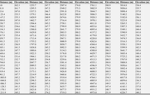
Table 1. The Elevation Profile For The Plateau.

Distance (m) Elevation (m) Distance (m) Elevation (m) Distance (m) Elevation (m) Distance (m) Elevation (m) Distance (m) Elevation (m)

0.0 262.3 1253.7 247.7 2507.4 274.0 3761.1 280.9 5014.8 254.4

41.8 261.7 1295.5 247.2 2549.2 275.3 3802.9 279.9 5056.6 255.7

83.6 247.0 1337.3 246.7 2591.0 275.6 3844.7 280.2 5098.4 257.0

125.4 253.5 1379.1 246.4 2632.8 280.9 3886.5 280.2 5140.2 256.6

167.2 255.3 1420.9 240.9 2674.6 279.9 3928.3 280.3 5182.0 256.1

209.0 247.0 1462.7 247.7 2716.4 280.2 3970.1 280.9 5223.8 254.0

250.7 253.5 1504.4 245.2 2758.1 280.3 4011.8 279.9 5265.5 251.1

292.5 254.6 1546.2 247.7 2799.9 280.9 4053.6 280.2 5307.3 248.0

334.3 245.8 1588.0 247.7 2841.7 279.9 4095.4 280.2 5349.1 244.4

376.1 239.9 1629.8 245.2 2883.5 280.2 4137.2 280.3 5390.9 241.0

417.9 235.4 1671.6 247.7 2925.3 280.3 4179.0 280.9 5432.7 238.5

459.7 231.6 1713.4 242.6 2967.1 280.9 4220.8 280.9 5474.5 236.0

501.5 232.7 1755.2 245.2 3008.9 279.9 4262.6 280.1 5516.3 237.4

543.3 236.9 1797.0 247.7 3050.7 280.2 4304.4 280.2 5558.1 239.9

585.1 241.5 1838.8 245.2 3092.5 280.3 4346.2 280.2 5599.9 242.5

626.9 247.7 1880.6 247.7 3134.3 280.9 4388.0 280.3 5641.7 245.6

668.6 245.2 1922.3 250.2 3176.0 279.9 4429.7 280.9 5683.4 248.4

710.4 231.6 1964.1 252.6 3217.8 280.2 4471.5 279.9 5725.2 248.3

752.2 232.7 2005.9 254.8 3259.6 280.3 4513.3 280.5 5767.0 248.2

794.0 231.6 2047.7 256.7 3301.4 280.9 4555.1 280.8 5808.8 245.2

835.8 232.7 2089.5 262.5 3343.2 280.9 4596.9 279.2 5850.6 241.7

877.6 236.9 2131.3 263.7 3385.0 279.9 4638.7 273.8 5892.4 238.8

919.4 241.5 2173.1 265.7 3426.8 280.2 4680.5 260.5 5934.2 236.6

961.2 247.7 2214.9 265.5 3468.6 280.3 4722.3 257.3 5976.0 235.1

1003.0 245.2 2256.7 266.4 3510.4 280.9 4764.1 254.3 6017.8 235.8

1044.8 232.7 2298.5 267.4 3552.2 279.9 4805.9 251.5 6059.6 236.3

1086.5 236.9 2340.2 269.3 3593.9 280.3 4847.6 249.5 6101.3 237.1

1128.3 241.5 2382.0 271.2 3635.7 280.9 4889.4 247.4 6143.1 237.8

1170.1 247.7 2423.8 272.1 3677.5 279.9 4931.2 248.7 6184.9 238.8

1211.9 245.2 2465.6 274.2 3719.3 280.3 4973.0 251.9 6226.7 240.2

Table 2. Rounded Edge Parameters For The Plateau Obstruction.

f (GHz) Frequency 6000

λ (m) Wavelength 0.05

S1 (m) The length of the tangent from the transmitter to the intersection point of the two tangent 4084.652326 S2 (m) the length of the tangent from the receiver to the intersection point of the two tangents 2142.842069

S3 (m) the length of the tangent from the receiver from the transmitter 6226.749177

d1 (m) the distance from the transmitter to the intersection point of the two tangents, that is point 4084.532567 d2 (m) the distance from the receiver to the intersection point of the two tangents 2142.177433

d (m) the distance from the transmitter to the receiver 6226.71

αt (radian) The angle the tangent line from the transmitter makes with the LOS 0.021359788 αr (radian) The angle the tangent line from the receiver makes with the LOS 0.011204902

α (radian) Sum of angles αt and αr 0.03256469

βα (radian) The angle the LOS makes with the horizontal 0.0035473

h (m) The LOS clearance height 45.76746032

D (m) the occultation distance 1922.34

V Diffraction parameter for all the methods except ITU-R method 7.721776507

V Diffraction parameter for the ITU-R P.526-13 Method 0.244008138

R1 (m) = The radius of the circle fitted in the vicinity of the hill vertex 48561.93427 R2 (m) = The radius of the circle fitted in the vicinity of the hill vertex using ITU method 12,658,123.28

Table 2 shows the values obtained for the key parameters of the rounded edge plateau obstruction. From Table 2, the path length (d) is 6226.71m. Also, the tangent from the transmitter and the tangent from the receiver intersected at a distance of 4084.532567m from the transmitter and a distance of 2142.177433 m from the receiver. The line of sight makes an angle of 0.0035473 radians with the horizontal. The LOS clearance height is 45.76746032m. The occultation distance is 1922.34m.

Table 3 shows the rounded edge radius computed by Hacking method and by ITU-R 526-13 method. The results in

Table 3 shows that the rounded edge radius computed by Hacking method is not affected by frequency. However, the rounded edge radius computed by ITU-R 526-13 method increases with frequency, as shown in figure 4. Also, the table 3 shows that the radius computed by the ITU-R 526-13 method exceed that computed by Hacking method by over 20,862%. The difference in radius also increases with increase in frequency.

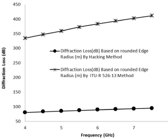
computed by Hacking method and also using the rounded edge radius computed by ITU-R 526-13 method. The results in Table 4 show that the diffraction loss determined using the rounded edge radius computed by ITU-R 526-13 method is much higher than that obtained using the rounded edge radius computed by

Hacking method. The percentage difference in diffraction loss in the two cases ranges from about 316% at 4GHz to about 337% at 8 GHz. In all, the ITU method for determining the rounded edge radius overestimate the value, especially for plateau with flat top that spans relatively large distance.

Table 3. Comparison Of The Effect Of Frequency On The Rounded Edge Radius Computed By Hacking Method and By ITU-R 526-13 Method.

Frequency (GHz) Rounded Edge Radius (m) Computed By Hacking Method

Rounded Edge Radius (m) Computed

By ITU-R 526-13 Method Percentage Difference in Radius (%)

4 59,031.42 12,374,693.37 20,862.89

4.5 59,031.42 12,374,693.37 20,862.89

5 59,031.42 12,374,693.37 20,862.89

5.5 59,031.42 12,658,123.28 21,343.03

6 59,031.42 12,658,123.28 21,343.03

6.5 59,031.42 12,658,123.28 21,343.03

7 59,031.42 12,658,123.28 21,343.03

7.5 59,031.42 12,658,123.28 21,343.03

8 59,031.42 12,954,399.00 21,844.92

Figure 4. Effect of frequency on the rounded edge radius computed by ITU-R 526-13 method.

Table 4. Comparison of the Effect of Frequency and The Rounded Edge on Diffraction Loss Over The rounded Edge.

Frequency (MHz) Diffraction Loss (dB) Based on rounded Edge Radius (m) By Hacking Method

Diffraction Loss (dB) Based on rounded Edge Radius (m) By ITU-R 526-13 Method

Percentage Difference in Diffraction Loss (%)

4 80.35494 334.9047 316.78

4.5 82.93134 347.6737 319.23

5 85.30611 359.5115 321.44

5.5 87.51339 373.149 326.39

6 89.57903 383.6205 328.25

6.5 91.52307 393.5154 329.96

7 93.36143 402.9067 331.56

7.5 95.10697 411.8535 333.04

8 96.77024 423.4129 337.54

Figure 5. Comparison Of The Effect Of Frequency and The Rounded Edge On Diffraction Loss Over Rounded Edge.

4. Conclusion

The effect of the radius of curvature on the diffraction loss of the rounded edge obstruction is presented. The study is conducted for C-band microwave link with a plateau in its path. Two different approaches are used to determine the radius of curvature of the rounded edged fitted to the plateau top. Among the two methods employed, the ITU-R 526-13 method overestimated the radius and also gave very high diffraction loss value for the plateau. In this wise, it can be concluded that the ITU-R 526-13 method is not particularly suitable for estimating the radius of curvature for the rounded edge when applied to a plateau. In addition, a more accurate method is required to estimate the radius of curvature for computing rounded edge diffraction loss.

References

[1] Seybold, J. S. (2005). Introduction to RF propagation. John Wiley & Sons.

[2] J. D. Parsons, The Mobile Radio Propagation Channel, 2nd ed., Wiley, West Sussex, 1992, pp. 45–46.

[3] B. McLarnon, VHF/UHF/Microwave Radio Propagation: A Primer for Digital Experimenters, www.tapr.org.

[4] W. C. Y. Lee, Mobile Communication Engineering, Theory and Applications, 2nd ed., McGraw-Hill, New York, 1998, pp. 147– 149.

[5] N. Blaunstein, Radio Propagation in Cellular Networks, Artech House, Norwood, MA, 2000, pp. 135–137.

[6] Willis, S. L. (2007). Investigation into long-range wireless sensor networks (Doctoral dissertation, James Cook University). [7] Lazaridis, P. I., Kasampalis, S., Zaharis, Z. D., Cosmas, J. P., Paunovska, L., & Glover, I. (2015, May). Longley-Rice model precision in case of multiple diffracting obstacles. In URSI Atlantic Conference, Canary Islands.

[8] Östlin, E. (2009). On Radio Wave Propagation Measurements and Modelling for Cellular Mobile Radio Networks.

[9] Kumar, K. A. M. (2011). Significance of Empirical and Physical Propagation Models to Calculate the Excess Path Loss.

Journal of Engineering Research and Studies, India.

[10] Malila, B., Falowo, O., & Ventura, N. (2016, April). Performance analysis of NLOS small cell backhaul using 17GHz point-to-point prototype radio. In Electrotechnical Conference (MELECON), 2016 18th Mediterranean (pp. 1-6). IEEE.

[11] Jicha, O., Pechac, P., Kvicera, V., & Grabner, M. (2013). Estimation of the radio refractivity gradient from diffraction loss measurements. IEEE Transactions on Geoscience and Remote Sensing, 51 (1), 12-18.

[12] Silva, F. S., Matos, L. J., Peres, F. A. C., & Siqueira, G. L. (2013, August). Coverage prediction models fitted to the signal measurements of digital TV in Brazilian cities. In Microwave & Optoelectronics Conference (IMOC), 2013 SBMO/IEEE MTT-S International (pp. 1-5). IEEE.

[13] Hacking, K. U. H. F. (1968). Propagation over rounded hills.

BBC Research Department. Research Report No. RA-21, 30. [14] International Telecommunication Union, “Recommendation

ITU-R P. 526-13: “Propagation by diffraction”, Geneva, 2013. [15] Seybold, J. S. (2005). Introduction to RF propagation. John

[16] Barué, G. (2008). Microwave engineering: land & space radiocommunications (Vol. 9). John Wiley & Sons.

[17] Jude, O. O., Jimoh, A. J., & Eunice, A. B. (2016). Software for Fresnel-Kirchoff Single Knife-Edge Diffraction Loss Model.

Mathematical and Software Engineering, 2 (2), 76-84.