2774 Int. J. Adv. Biol. Biom. Res, 2014; 2 (11), 2774-2778
*Corresponding Author: Valiollah Rasoli, Ph.D. Member, Agricultural and Natural Resources Research Center of Qazvin, Qazvin, Iran
A R T I C L E I N F O A B S T R A C T
Article history: Received: 06 August, 2014 Revised: 29 September, 2014 Accepted:19 October, 2014 ePublished: 30 November, 2014
Key words: Path analysis Grapevine
Logarithmic analysis
Yield stability
1.INTRODUCTION
Grapevine (Vitis vinifera L.) is one of the most important
horticultural crops in the world and Iran. According to the reports of FAO (2009), grapevine cultivated area was 7,598,570 and 307,721 hectares in the world and Iran, respectively. World production of grape is about 67.5 million tons. Iran with 1.9 million tons production is located in seventh of world ranking (FAO, 2009). Main yield components have the most importance in many
plant breeding research programs. Grapevine breeders’
aim is to increase the final yield by selection of main yield
components such as number of cluster per plant, number of berry per cluster and berry mean weight. For this reason, they want to know which one of the main yield components has the most genetic contribution in complicated yield trait. A complicated or complex trait such as yield, can be define as trait which its variations
are identified by variations of its components
(Farshadfar, 1999). Using of recombinative heterosis has been suggested for identification of genetic contribution of each yield components in final yield (Sparnaaij and Bos, 1993 ). This method will has less efficient in fruit trees because access to new generations requires several IJABBR- 2014- eISSN: 2322-4827
International Journal of Advanced Biological and Biomedical Research Journal homepage: www.ijabbr.com
Original Article
Genetic Contribution of Grapevine (
Vitis Vinifera
L.) Main Yield Components in Final Yield
Valiollah Rasoli*1, Ezatollah Farshadfar2, Jafar Ahmadi3
1Ph.D. Member, Agricultural and Natural Resources Research Center of Qazvin, Qazvin, Iran 2Professor, Faculty of Agriculture, Razi University, Kermanshah, Iran
3Associated Professor, Imam Khomeini International University, Qazvin, Iran
Objective: Yield components and genetic contribution have the most important in final yield and breeding programs of crop plants. For this purpose, 20 varieties of grapevines with Russia origin were evaluated in Urmia and Takestan research station (under full
irrigation and drought stress). Methods: Twenty grapevine genotypes were evaluated in
Urmia and Takestan research station (under full irrigation and drought stress) in randomized complete blocks design with three replications and three plants in each plot. Number of cluster per plant, Number of berry per cluster, berry weight and yield of each plants were recorded. Compound and logarithmic analysis of variance, variance of genetic components and environmental interactions were presented by multiplicative
three environmental and genotypic elements. Results: Results indicated that number of
cluster per plant had the highest genetic contribution in final yield and also had the most sensitivity and variation in different environments. Direct effect of number of cluster per
plant in final yield was higher than other studied traits. V3 value was higher than V2 and
V2was higher than V1, therefore sequence of manifestation of yield components were
number of cluster per plant, number of berry per cluster and berry weight, respectively.
Environmental components of interactions were indicated that absolute value of r1 was
higher than r2 and r3. Conclusion: These results indicated that number of cluster per
years in sexual hybridization. Huhn (1979) suggested the method of stability analysis based on principal components. In this method, logarithmic variance analysis and path analysis are used in different
environmental conditions. According to these
researchers, yield of plants is a complex trait which its components have developed during plant growth period. Therefore different environmental factors will have different effects on these traits.
In this article, path analysis and genetic contribution of grapevine main yield components were identified on the basis of developmental growth components in different environmental conditions.
2. MATERIALS AND METHODS
In this study, 20 grapevine genotypes with Russian origin were evaluated in one location of Urmia and two locations of Takestan (under full irrigation and drought stress). This research was performed in randomized complete blocks design with three replications and three plants in each plot in 2012. Fruit yield (kg/plant), number of cluster per plant, number of berry per cluster and berry mean weight were recorded. Compound analysis of variance was done for yield and yield components. Path analysis in different environment was done and genetic contribution of yield components in final yield were identified. In this model, firstly, it is assumed that growth chronologically of main yield components are in this way that the number of clusters per plant (X), the number of berry per cluster (Y) the berry weight (Z) and yield (W) that obtain by multiplying of these components (W = X × Y × Z). Secondly it is assumed that environmental resources can be divided into three independent components such as R1, R2 and R3 that each group is stimulating the growth of other traits in growth period and then path diagram was drawn on the basis of this concept.
In order to discover the relationship between these three independent environmental groups in path analysis, it is
assumed that ñxy, ñxz, ñyz, ñxw, ñ ywñ and ñzw are
correlation coefficients between yield and its main
components. Also a1 to a6 are path coefficients. Therefore,
the following relationships will be:
ñxy= a1 ñxz= a2+a1a3 ñyz= a3+a1a2
ñxw=a4+a1a5+a2a6+a1a3a6 ñyw= a5+a1a4+a3a6+a1a2a6 ñyz=a6+a2a4+a3a5+a1a3a4+a1a2a5
Six path coefficients can be obtained by solving the following equations simultaneously.
A= ∆-1ñ
A'=(a1 a2 a3 a4 a5 a6)
ñ'= ( ñxy ñxz ñyz ñxw ñyw ñzw )
U1, U2 and U3 are the coefficients from R1 to X, R2 to Y and
R3 to Z, respectively as follow:
U1= ±1
U2= ± (1-a12)0.5
U3= ± (1- a2ñxy- a3 ñyz)0.5
These coefficients can be positive or negative according to the used scale. Here, positive coefficients were used. If
W, r1, r2 and r3 represent yield and three different
environments, respectively, then the following equation will be established.
W= V1'r1' + V2'r2' + V3'r3' +e'
In this equation, V1', V2' and V3' are path coefficients from
R1, R2 and R3 to yield (W), respectively, and e' is residual.
V1', V2' and V3'can be obtained by the following formulas:
V1'= U1 (a4 + a1a5 + a2a6 + a1a3a6)= U1ñxw
V2'= U2 (a3a6 + a5)
V3'= U3a6
Yield of ith genotype can be obtained by the following
formula in jth environment:
W= ìwi + V1ir1j + V2ir2j + V3ir3j + e'
In this formula, Vgi=V'giówi is for g=1, 2, 3 … and ó2wi is the
yield variance of ith genotype. Also this formula is a
mathematical model for the observed yield (Wij). This
model includes genotypic mean effect (ìwi), three
multiplicative components of interactions of genotype and environment (including three genotypic components
V1i, V2i, V3i and three environmental components r1j, r2j
and r3j) and error component (eij). Each of the three
genotypic components identifies the contribution of the three components X, Y and Z in the interaction of genotype and environment. Also, each of the three environmental components indicates contribution of these components in the environment. In logarithmic
model, if Log (Y) = Log (x1) + Log (x2) + Log (x3),then
covariance of yield and its main components will be Ci=
cov[Log (w), Log (x,y,z)] and ó2(Y)=Óc
i (Tai, 1975, Tai,
1979, Tai et al., 1994 and Huhn, 1979).
3. RESULT AND DISCUSSION
of genes controlling this trait is higher and the contribution of each gene to control it will be lower. Therefore it has a high environmental impact. Covariance
of yield and its main components and values of Ci had
been estimated in table 3 on the basis of logarithmic model for each genotype.
Table 1.
Variance analysis of yield and its component in different environments.
Source of variation Degree of freedom
Number of cluster per plant
Number of berry per cluster
Berry weight
(g) Yield (kg/p)
Environment 2 3491.3** 29240.1** 10.21** 1301.89** Replication/ Environment 6 92.2 367.2 0.02 36.01
Genotype 19 2178.7** 13382.8** 9.7** 257.64** Genotype × Environment 38 265.7** 3008.1** 1.4** 96.66**
Error 114 130.9 748.5 0.07 17.46
**
:
significance at á= 0.01Table 2.
Genetically parameters estimation of yield and its component.
parameters Number of
cluster per plant
Number of berry per cluster
Berry weight
(g) Yield (kg/p)
Coefficient of Variation (%) 9.5 15.8 8.4 11.2 Phenotypic variance 343.46 1901.24 0.99 35.35
Genotypic variance 212.56 1152.74 0.92 17.89 Environmental variance 130.90 748.50 0.07 17.46
Variance of
Genotype × Environment 44.93 753.20 0.44 26.40
Broad-sense heritability (%) 54.7 43.4 64.3 29
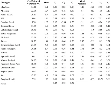
Table 3.
Genotypic components (V1, V2 and V3) and covariance of yield with its components in different environments.
Genotypes Coefficient of
Variation (%) Mean C1 C2 C3
Yield
variance V1 V2 V3
Ulskibiser 14.42 9.4 0.26 0.83 0.10 1.19 -1.68 3.75 3.46
Aligoneh 33.64 3.7 0.39 0.16 0.38 .81 -0.53 1.19 1.10
Ramfi TCXA 20.19 5.7 0.44 0.39 -0.03 .72 -0.81 1.82 1.68
46X 9.04 14.1 0.53 0.38 0.12 1.04 -3.14 7.01 6.47
Gezgiski Ramfi 5.70 12.7 0.12 -0.04 0.23 .31 -1.91 4.26 3.93
Superan Bulgar 11.67 9.6 0.37 0.35 0.30 .99 -2.50 5.60 5.17
Uzbakestan Moscat 10.46 10.1 0.35 0.34 0.05 .71 -1.19 2.66 2.46
Bobili Magaracha 48.77 2.8 0.21 0.50 0.47 1.18 -0.31 0.69 0.64
Bli Ramfi 12.29 8.1 0.32 -0.05 0.29 .56 -1.38 3.08 2.84
Skieve 10.73 16.0 0.93 0.66 0.56 2.15 -2.53 5.65 5.21
Tambuzh Shaki Ramfi 21.95 5.0 0.25 0.29 0.14 .68 -0.88 1.96 1.81
Ramfi ezdangara 20.65 6.5 0.68 0.38 0.41 1.46 -1.80 4.02 3.71
Muscat 6.51 16.0 0.01 0.65 0.20 .87 -2.48 5.54 5.11
Apozoski Ramfi 8.01 22.4 0.79 0.57 0.75 2.11 -4.46 9.97 9.20
Muscat Ruskovi 16.83 6.5 0.30 -0.05 0.49 .74 -0.65 1.45 1.34
Kishmish Ramfi Azos 18.64 8.4 1.02 0.44 0.14 1.60 -1.03 2.30 2.12
Ukranski Ramfi 8.96 9.1 0.07 0.42 0.21 .55 -2.44 5.46 5.04
Negrod yalon 8.98 10.8 0.51 0.08 -0.04 .56 -2.23 4.98 4.60
X45 17.55 4.5 0.19 0.04 0.09 .32 -1.11 2.48 2.29
Anapiski Ramfli 7.72 19.9 0.85 0.63 0.59 2.06 -4.79 10.71 9.88
Covariance of yield with number of cluster per plant (C1)
was higher than covariance of yield with other yield components in many genotypes. Also, these values were positive in all genotypes. Mean of covariance of yield with number of cluster per plant (0.42) was higher than means of covariance of yield with other yield
components (Table 3). Positive and high value of C1
represented the fact that genetic contribution of number of clusters per plant has the higher impact on increase of final yield than the other components. Also, variations of yield in different environments and interaction between yield and environment were most affected by this trait in all grapevine genotypes but Gezgiski Ramfi, Muscat and
Ukranski Ramfi (Table 3). Negative values of Ci in number
of berry per cluster and mean weight of berry in some genotypes indicated the lower genetics contribution of these traits in final yield.
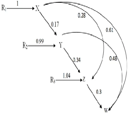
In path analysis of yield and its components in different environments (Fig. 1), direct effect of number of cluster per plant (0.61) was higher than direct effects of number of berry per cluster (0.48) and berry mean weight (0.3) in final yield. On the other hand, indirect effect of number of cluster per plant by number of berry per cluster (0.17) and berry mean weight (0.28) path way were lower than their direct effects in final yield. These results were confirmed the findings of logarithmic analysis and high contribution of number of cluster per plant in final yield.
Fig. 1. Path analysis of grapevine yield and its components in
different environments
Mean of yield and genotypic components (V1, V2 andV3)
indicated that V3 and V2 values were higher than V1 values
(Table 3). Also, difference between V3 and V2 values was
very low. On the other word, number of clusters per plant was earlier than other yield components in grapevine. Also genotypic components values of Anapiski Ramfli and Apozoski Ramfi were higher than genotypic components values of other genotypes. These genotypes will have higher yield than other genotypes in ideal environments.
This case was also proved by lower percentage of variation coefficients of these genotypes (table 2). Genotypes Aligoneh and Bobili Magaracha will have more stable yield than other genotypes because of the lower
genotypic components values and percentage of
variation coefficients in different environments (table 3) (Farshadfar, 2010). Estimating of three environmental
components of interactions r1, r2 and r3 had been shown
in table 4. Environmental components of interactions
were indicated that absolute value of r1 was higher than
r2 andr3 in all environments. This indicated that number
of cluster per plant had the highest sensitivity in different environments. Drastic environmental changes will have
more different impact on this trait. Effects of
environmental variations on berry weight was low and
therefore this trait had less sensitivity to the
environmental changes (table 4).
Table 4.
Environmental components estimation (r1, r2 and r3) of
variety and Environment Interaction. Environmental
component Takestan
Takestan
(drought stress) Urmia
r1 1.8 0.2 0.4
r2 0.6 0.0 0.3
r3 0.4 0.1 0.4
Tai ( 1979 ) surveyed adaptability of potato yield components in different environments by path analysis
and concluded that r3 was higher and more variable than
r1 and r2 in different environments. Also Tai et al. ( 1994)
investigated sensitivity to temperature index in potato yield components and concluded that environmental
component r4 was higher than the others. Farshadfar
(1999) reported that, genetic contribution of seed number per spike in genotype and environment interaction was more than genetic contribution of spike per plant and grain weight in wheat chromosome addition lines. Also he indicated that sensitivity of seed per spike to environmental variation was lower than other two components. Therefore the seed per spike had the most important role in phenotypic stability of wheat
in different environments. Also he identified
chromosomal genes location of genotype and
environment interaction by this method. These results were similar to the findings of the present study, because the first multiplicative component of yield had the highest genetic contribution in final yield.
Phenotypic stability of bread wheat was investigated by using path analysis method in drought stress and
complete irrigation by Farshadfar et al. (2012). They
higher genetic contribution of second multiplicative component of final yield. Therefore it can be concluded that the genetic contribution of yield components will be different in plant species. Also this result was confirmed
by Farshadfar et al. (2013). In their research, number of
seed per pod of pea (the second multiplicative component) had the highest genetic contribution in final yield and its non-stability in different environmental conditions.
Path analysis of grapevine yield and its main components
was conducted only by (Fanizza et al. (2005). In their
study, complete and partial correlation method was used for yield path analysis in an environment. They concluded that number of cluster per plant, number of berry per cluster and berry weight had significant positive correlation with yield, but number of cluster per plant had significant negative correlation with number of berry per cluster and berry weight. This method is not able to determine the genetic contribution of main yield components in yield variance and also will not show sensitivity of main yield components in different environmental conditions. While the present study, provided the data of three different environment about genetic contribution which determine the main yield components in yield variance that is the strong point of this research. Other applications of logarithmic and path analysis methods in different environments is the yield
stability analysis of each cultivar in different
environmental conditions and determination of cultivars with sustainable yield for each environment. It also has a high capability in selecting parents for heterosis breeding (Farshadfar, 2010).
CONCLUSION
This research indicated that number of cluster per plant had the highest genetic contribution, variations and sensitivity in final yield in different environmental conditions. Therefore number of cluster per plant will has more importance than other yield components in selection of high yield grapevine genotypes in ideal environments. Also number of berry per cluster and berry weight will have more importance in selection of grapevine genotypes with higher stable yield indifferent environmental conditions. Findings of this research showed that the high variance in yield had correlation with high variance of main yield components. If the plant which is under study shows great flexibility in the yield structure, it may increase one component with decrease in another component which indicates the negative covariance among yield components. Therefore the component that has more variation (high variance) but it can be compensated by other components (negative covariance), it has little effect on the yield variance. This
case is seen in the low Ci value of that component. One of
the advantages of logarithmic method is the
independence of variance and covariance with
measurement units. Therefore variance of different traits will be comparable with different measurement units.
REFERENCES
Fanizza, G., Lamaj, F., Costantini, L., Chaabane, R., Grando, M.S. (2005). QTL analysis for fruit yield components in table grapes (Vitis vinifera). Theor. Appl. Genet, 111: 658-665.
FAO, 2009. Statistical database.
Farshadfar, E. (1999). Path analysis of genotype and
environment interactions in wheat chromosome
substitution lines. Iran agricultural science journal, 30: 665-671.
Farshadfar, E. (2010). New discussions in biometrical genetics. Kermansha Islamic Azad University Press II, 1174- 1219.
Farshadfar, E., Mahtabi, E., Jowkar, M.M. (2013). Evaluation of genotype × environment interaction in chickpea genotypes using path analysis. International journal of Advanced Biological and Biomedical Research, 1: 583-590.
Farshadfar, E., Rasoli, V., Mohammadi, R., Veisi, Z. (2012). Path analysis of phenotypic stability and drought
tolerance in bread wheat (Triticum aestivum L.). Int. J.
Plant Breed., 6:106-112.
Huhn, M. (1979). Beitrage zur erfassung der
phanotypischen stabilitat. I. Vorschlag einiger auf Ranginformationnen beruhenden stabilitatsparjameter. EDV Medizin Biol., 10: 112-117.
Sparnaaij, L.D., Bos, I. (1993). Component analysis of complex characters in plant breeding. Euphytica, 70: 225-235.
Tai, G.C.C. (1975). Analysis of genotype environment interactions based on the method of path coefficient analysis. Canadian Journal of Genetics and Cytology, 17: 141-149.
Tai, G.C.C. (1979). Analysis of genotype environment interaction of potato yield. Crop Sci., 19: 434 - 438.