Lung Disease Classification using GLCM and Deep Features from Different Deep Learning Architectures with Principal Component Analysis

(1)

IJIE

Journal homepage: http://penerbit.uthm.edu.my/ojs/index.php/ijie

The International

Journal of

Integrated

Engineering

Lung Disease Classification using GLCM and Deep Features

from Different Deep Learning Architectures with Principal

Component Analysis

Joel Than Chia Ming

1*

, Norliza Mohd Noor

2

, Omar Mohd Rijal

3

, Rosminah M.

Kassim

4

_{, Ashari Yunus}

5

1&2_{Razak Faculty of Technology & Informatics,}

Universiti Teknologi Malaysia, Jalan Semarak, Kuala Lumpur, 54100, MALAYSIA

3_{Institute of Mathematical Science,}

University of Malaya, Lembah Pantai, Kuala Lumpur, 50603, MALAYSIA

4_{Dept of Diagnostic Imaging,}

Kuala Lumpur Hospital,Jalan Pahang, Kuala Lumpur, 50586, MALAYSIA

4_{Institute of Respiratory Medicine,}

Kuala Lumpur Hospital,Jalan Pahang, Kuala Lumpur, 50586, MALAYSIA

*Corresponding Author

DOI: https://doi.org/10.30880/ijie.2018.10.07.008

Received 30 October 2018; Accepted 18 November 2018; Available online 30 November 2018

1. Introduction

Lung diseases such as emphysema, pneumonia and chronic obstructive pulmonary disease (COPD) contribute as the third leading causes of death today behind ischemic heart diseases and stroke (Lung, Institute, & others, 2012). In Malaysia particularly, most of the lung diseases are diagnosed at the advanced stage (IV) (“Malaysia: Lung Disease. In World Health

Abstract: Lung disease classification is an important stage in implementing a Computer Aided Diagnosis (CADx) system. CADx systems can aid doctors as a second rater to increase diagnostic accuracy for medical applications. It has also potential to reduce waiting time and increasing patient throughput when hospitals high workload. Conventional lung classification systems utilize textural features. However textural features may not be enough to describe properties of an image. Deep features are an emerging source of features that can combat the weaknesses of textural features. The goal of this study is to propose a lung disease classification framework using deep features from five different deep networks and comparing its results with the conventional Gray-level Co-occurrence Matrix (GLCM). This study used a dataset of 81 diseased and 15 normal patients with five levels of High Resolution Computed Tomography (HRCT) slices. A comparison of five different deep learning networks namely, Alexnet, VGG16, VGG19, Res50 and Res101, with textural features from Gray-level Co-occurrence Matrix (GLCM) was performed. This study used a K-fold validation protocol with K= 2, 3, 5 and 10. This study also compared using five classifiers; Decision Tree, Support Vector Machine, Linear Discriminant Analysis, Regression and k-nearest neighbor (k-NN) classifiers. The usage of PCA increased the classification accuracy from 92.01% to 97.40% when using k-NN classifier. This was achieved with only using 14 features instead of the initial 1000 features. Using SVM classifier, a maximum accuracy of 100% was achieved when using all five of the deep learning features. Thus deep features show a promising application for classifying diseased and normal lungs.

(2)

Rankings,” 2012). This shows an alarming situation where there is an imbalance of late diagnosis of lung diseases in advanced stages as compared to early stages. Later diagnosis decreases the effectiveness of treatment plans and thus decreasing the chance of recovery. However with earlier detection, better prognosis and treatment can be administered to increase the rate of survival and quality of life post treatment. The benefits of having earlier diagnosis and treatment coupled with the current condition of late diagnosis of lung diseases show the relevance of current research works in finding possible methods to classify diseases quicker for better treatment planning and execution. This very reason propels studies to investigate, develop and propose Computer Aided Diagnosis (CADx) systems. CADx systems have also shown improvement in breast cancer diagnosis (Jiang et al., 1999). There is a growing demand for CADx systems however its implementation into ready healthcare based systems is still not complete (Doi, 2007).

The bulk of most past research on supervised learning and classification of diseases have focused more on textural features. Textural features have shown their effectiveness in classification potential in past research (A Han et al., 2014; Cirujeda et al., 2016; Shrivastava, Londhe, Sonawane, & Suri, 2016). One of the earliest and popular method is Graylevel Co-occurrence Matrix (GLCM) (Haralick, Shanmugam, & Dinstein, 1973). GLCM has shown to be useful in classification lungs classification (Huber, Nagarajan, Leinsinger, Ray, & Wismuller, 2010; Wang, Li, & Li, 2009). The most recent powerful textural features used for classification are Gabor Transform and Riesz Transform. Both these two transforms provide a robust description of an image. This is because both feature extraction methods provide scalability and steerability option to describe an image (Than et al., 2017). Gabor has shown its capability to classify various fields such as lung (Mitani et al., 2000), fingerprint (Lee & Wang, 1999), face (See, Noor, Low, & Liew, 2017) and even hand writing (Annanurov & Noor, 2017). Riesz Transform has shown its potential in classifying diseased lungs (Depeursinge & Rodriguez, 2011) as well as different lung tissues (Cirujeda et al., 2016, 2015). The textural method of feature extraction has shown its potential in many different fields and are a common approach to be selected as a feature extraction technique for classification.

However conventional machine-learning methods were inadequate in processing natural data in their raw form (LeCun, Bengio, & Hinton, 2015). This weakness has caused the need for unconventional techniques such as deep learning. In recent works, deep features have shown a more promising way forward. This is because it shows a new type of robust and wide depth of features previously unavailable. Deep learning is a form of representational learning, where raw data is fed in to a network automatically discover the representations needed for detection or classification (LeCun et al., 2015). However the major drawback of such methods is the training time and computational strain of using large feature sets.

The main purpose of this study is to propose a classification system to classify normal and diseased lungs using deep features from different deep learning architectures. This study also introduces the use of Principal Component Analysis (PCA) with deep features and compare the results with several different classifiers to show the effectiveness of deep features and to combat the previously mentioned computational strain of large feature sets.

2. Materials

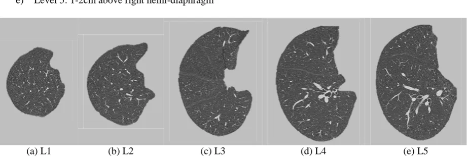
High Resolution Computed Tomography (HRCT) of the thorax region were obtained retrospectively from Hospital Kuala Lumpur. For this study, HRCT slices from 81 diseased and 15 normal patients were used. Each slice was sized at 512 x 512 pixels. These patients had lung diseases such as emphysema and Interstitial Lung Disease (ILD). There were 48 male and 48 female patients. A senior radiologist was tasked to choose the five levels or slices of each patient. Example of these five levels are shown in Fig. 1 and Fig. 2. These five levels correspond to specific anatomic landmarks as below where diseases are usually seen and evaluated in a patient’s scan (Chia et al., 2014; Kazerooni et al., 1997);

a) Level 1: aortic arch b) Level 2: trachea carina c) Level 3: pulmonary hilar

d) Level 4: pulmonary venous confluence e) Level 5: 1-2cm above right hemi-diaphragm

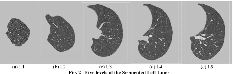
(a) L1 (b) L2 (c) L3 (d) L4 (e) L5

(3)

(a) L1 (b) L2 (c) L3 (d) L4 (e) L5 Fig. 2 - Five levels of the Segmented Left Lung.

3. Methodology

The overview of this study is shown in Fig. 3. The input of the system was a HRCT slice which is then segmented. The segmentation used here was a previously introduced segmentation method using thresholding and texture applications. The segmented lungs were then pre-processed to fit the deep learning architectures’ input formats. Since the segmented lungs are in DICOM format, they have are only single channel and at the size of 512 x 512 pixels. Pre-processing deals with these channels and size discrepancies. The new preprocessed image was then fed into the feature extraction stage. After this, feature selection and feature transformation in the form of Principal Component Analysis (PCA) was done to reduce the number of features available. The new features were then fed into the classification stage. The classification stage aims to classify two classes which are diseased and normal lungs. The predicted lung classes were then compared with the ground truth provided by the medical diagnosis.

Fig. 3 - Overview of stages for lung disease classification.

3.1 Segmentation

The segmentation system used follows previous works that featured a combination of segmentation techniques and its overview is shown in Fig. 4 (Chia et al., 2014; Noor et al., 2013, 2015). The lung segmentation methods can be divided into the primary and the secondary segmentation. The primary segmentation used a two types of thresholding in the form of Otsu thresholding and an empirical threshold with morphology operations (Otsu, 1979). The secondary segmentation used an entropy filter coupled with morphology operations. The similarity check feedback allows for spotting errors of segmentation from the primary segmentation. Note that this study does not focus on the development of segmentation method but more on the usage of a deep learning architecture as a feature extraction tool and the usage of PCA for feature selection.

(4)

3.2 Preprocessing

The segmented lungs were then pre-processed to allow it to be suitable as inputs for the deep learning architecture. This includes resizing the image from 512 x 512 to the designated input of each architecture. Besides that the grayscale image is also converted to a RGB image format as well. For this study, the DICOM image was displayed in a figure and the three channel information were extracted and saved as a new three channel image. An important note is that the preprocessing stage is only applied for the deep features and not required when extracting GLCM features. This was done because of the restrictions of input for the deep learning networks.

3.3 Feature Extraction

Features help represent certain characteristics of an image that are helpful in providing beneficial information for making decisions on which classes a particular image belongs to. The feature extraction stage of this study can be said to involve two main features. The first feature set used in this study was the readily available and mainly used Gray-level Co-occurrence Matrix (GLCM). The second feature set involves five different deep learning architectures that produces 1000 features each. This study compares the widely accepted method GLCM with a new emerging deep features. As stated before deep features can make up for the weakness of textural methods by offering information from the raw form of an image.

3.3.1 GLCM

This study used Gray-level Co-occurrence Matrix (GLCM) as a type of feature. GLCM is one of the widely used feature extraction methods in medical image classification. There are primarily four features of GLCM which are contrast (Con), correlation (Cor), Energy (E) and Homogeneity (H). The features were calculated according Eq. 1 – 4 (Haralick et al., 1973). The implementation of the GLCM method is similar with the author previous study (Ming, Rijal, Kassim, Yunus, & Noor, 2017).

 



  

    N i N j j i P j i 1 1 , 2

Con  













 





x y



N

i N

j

y x j Pi j

i   , / 

Cor 1 1



       



 

   N i N j j i P 1 1 ,

E  





 





     N i N j j i j i P 1 1 1 / ,

H  

where P is the gray level matrix, i and j represent the x and y coordinate of the image, μx and σyrepresent mean and the

standard deviation of the rows of a GLCM where as μy and σyrepresent mean and the standard deviation of the columns

of a GLCM, and respectively.

3.3.2 Deep Features

The inspiration of this work comes from studies of various authors that managed to use a deep learning approach to form a new set of deep features for various classification purposes and modalities such as ocular (Awais, Muller, & Meriaudeau, 2017), lung (Hooda, Sofat, Kaur, Mittal, & Meriaudeau, 2017), and even in leaf patterns (Prasad, 2017). Deep features are the outputs extracted from a fully connected (FC) layer of a pre-trained deep learning architecture. This method of feature extraction can be said to be a form of transfer learning, since there is a transfer from a pre-existing and pre-trained network. In this study only layers that produce 1000 outputs are used to provide an even comparison between these five architectures. This was chosen so that the computational strain will not be too great as compared to using the full features (4096 features). The large number of features produced offers a rich and robust information that previously was not available from textural analysis methods. Images undergo convolution to produce a numeric output that allows a classifier to make a decision on the class of an image. The five deep learning architectures used in this study are Alexnet, VGG16, VGG19, Resnet50 and Resnet101 which are growing in popularity and versatility. This study used pre-trained networks downloadable on the Matlab repository and compatible with Matlab2017a onwards.

3.3.2.1 Alexnet

(5)

arrow in Fig. 5. The output from this layer produces 1000 features. This layer was chosen so that the number of features will be consistent with the other deep learning architectures.

Fig. 5 - Representation Overview of Layers (green) and corresponding sizes (blue) in Alexnet

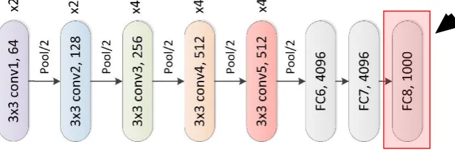
3.3.2.2 VGG16 and VGG19

Secondly, this study used VGG-16 as the feature extraction method. Similarly to Alexnet, VGG-16 uses a convolution neural network (Simonyan & Zisserman, 2014). However the difference is that depth to 16 weight layers, which is substantially deeper than what has been used in the prior deep learning architectures. This increase in layers is because of the addition of repeated blocks. VGG16 had layers that repeated twice (conv1 & conv2) and three times (conv3 – conv5). It was designed with small 3×3 filters in all convolutional layers to decrease the number of parameters in very deep networks. The main blocks are similar to that of Alexnet in Figure 3, however the depths within each block are different. The input image of VGG-16 uses an image that must be sized at 224 x 224 in RGB format. The overview of VGG16 and its layers are shown in Fig. 6. Features are extracted from the FC8 layer that yields 1000 numeric outputs. This layer is the red box and black arrow in Fig. 6

Fig. 6 - Representation Overview of Different Layers of VGG16.

This study also used VGG-19 which is an extension of VGG-16. This architecture has an increased depth to 19 weight layers. The difference is seen in Fig. 7 where the green, orange and red blocks are repeated four times instead of only three times in VGG-16. As before, the features are extracted from the FC8 layer which yields 1000 numeric outputs. The input image of VGG-19 is similar as VGG-16, which is an image that must be sized at 224 x 224 in RGB format.

(6)

3.3.2.3 Resnet50 and Resnet101

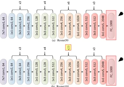
Resnet is an abbreviation for Residual Network where residual learning is utilized. Just like VGG16 and VGG19 the numbers in the name of Resnet50 and Resnet101 indicate the number of layers of the network which are 50 and 101 respectively. After the inception of Alexnet, there was a race to build deeper networks with more layers such as Googlenet with 22 layers. However researches begin to question the depth of this deeper networks where the initial information from the first formative layers are lost down the line. Another problem arises as the depth in increased accuracy begins saturating and eventually degrading. This inspired the use of residual learning that aims to combat both these problems (He, Zhang, Ren, & Sun, 2016).

Residual learning as the name indicates focuses on the residual of each layer so that information will not be lost. Generally residual can be represented as the subtraction of feature learned from input of that layer. Resnet does this by performing a shortcut connection and element-wise addition for every few blocks. The shortcut connection directly connects the input of nth_{layer to some (n+x)}th _{layer which is the end of few blocks (He et al., 2016). The two networks} used for this study are shown in Fig. 8. Note that the difference between both is located in the yellow box for Resnet101 marked Fig. 8(b) where the orange blocks are repeated 23 times instead of six times in Resnet50 in Fig. 8(a). There is only one fully connected layer in these two networks and its output is 1000 numeric outputs as indicated by the two black arrows in Fig. 8.

(a) Resnet50

(b) Resnet101

Fig. 8 - Representation Overview of Different Layers of Resnet50 and Resnet101.

3.4 Feature Selection

Feature selection was done using Principal Component Analysis (PCA). PCA is a mathematical approach to reduce the dimensionality and compress the amount of features available (Wold, Esbensen, & Geladi, 1987). This is achieved by transforming to a new set of features called the principal components (PC)s, which are uncorrelated, These PCs are in a specific sequence where the initial PCs have the most variation when compared to the original features. The longer the sequence the less variation the PC has to the original features (Jolliffe, 2011).

3.5 Classification

(7)

the data into a training dataset and testing dataset. The training dataset is (k-1)/k fraction of the whole dataset whereas the testing set is 1/k fraction of the whole dataset. Note that these two datasets do not have shared values however have the same proportion of class labels.

3.6 Classification Performance

For this study we used True Positive (TP), False Positive (FP), True Negative (TN), and False Negative (FN) as the initial indicators to define the classification performance. For the application of this study, TP was the rate of occurrences that the system was able to classify diseased lungs as diseased lungs. FP was the rate when normal lungs were identified as diseased lungs. TN was the rate of normal lungs being correctly identified. FN was the rate when diseased lungs were identified as normal lungs. Now we can define the performance measures used. We used sensitivity (SEN) Eq. 5, specificity (SP) Eq. 6, positive predictive value (PPV) Eq. 7, negative predictive value (NPV) Eq. 8, and accuracy (ACC) Eq. 9. ROC curve’s vertical axis represents sensitivity and its horizontal axis represents (100%-Specificity) (Shrivastava et al., 2016). Calculations were done following a previous study (Ming et al., 2017). Matthew’s Correlation Coefficient (MCC) was also calculated according to Eq. 10. The values of MCC can range from -1 to 1. When values were closer to 1, features can be said to have a positive relationship to classification of class labels, where as if it is closer to -1, features can be said to have a negative relationship to the true class labels. MCC is particularly beneficial when classes are imbalanced. ACC may give a bias result especially when one class outnumbers another class.

 SEN 100%

 

FN TP

TP _ _

 SPE 100%

 

TN FP

TN _ _

 PPV 100%

 

FP TP

TP _ _

 NPV 100%

 

FN TN

TN _ _

 ACC 100%

     FP TN FN TP TN

TP _ _

 ) )( )( )( ( M FN TN FP TN FN TP FN TP FN FP TN TP CC          

4. Experiment Protocols

For this study, the experiments that were carried out can be split to three protocols and are listed in this section. These three portions of experiments were carried to evaluate firstly the difference in classification performance between deep features and GLCM. Secondly the effect of adding PCA to deep features were also shown in terms of classification performance. Finally the variation of number of Principal Components on the classification accuracy was also studied.

4.1 Comparison of Deep Features and GLCM

This experiment focuses on the features extracted from different deep learning architectures with GLCM features. For this portion of the study, a decision tree classifier was used to classify the diseased and normal lungs with 10-fold validation. This was repeated with Support Vector Machine (SVM) classifier to see the increase in accuracy. The classification performance of all features were displayed and compared. The ROC plots were also compared. The computational time of feature extraction for the deep learning features were also calculated. Since all the deep learning features produced very high accuracies with SVM, the computational time matters especially in the real world applications where there are very large data to be analyzed. Thus the deep features with the least computational time was chosen for the next experiment.

4.2 Analysis of Deep Features + PCA

Next we paired the deep features that required the least computational time with PCA and compared its classification accuracy with and without PCA. An important note, PCA features were chosen based on the 95% variance where features that contribute to 95% difference between the new transformed PCA features and the original 1000 deep learning features. This experiment was carried out for four different K-fold values which were K=2, 3, 5 and 10. We also used five different classifiers for this experiment which were Decision Tree, Support Vector Machine, Linear Discriminant Analysis (LDA), Regression and k-Nearest Neighbor (k-NN).

4.3 Analysis of Principal Components on Classification Accuracy

(8)

The ideal amount of features show that the 95% approach may not be the best fit solution for different classifiers and situation.

5. Results

In this results section the results of the three experiment protocols were shown. It was encouraging that the algorithm of using deep features produced high accuracies with and also without PCA. These three situations highlight how we can improve the accuracy of classification by improving the classifiers and the amount of features available.

5.1 Initial Comparison of Deep Features and GLCM

The classification of using the five different deep features and GLCM are shown in Table 1. The results were obtained when using Decision Tree classifier with a 10-fold validation. The highest accuracy was achieved using Res50 with an accuracy of 96.33%. The lowest accuracy was obtained using GLCM at 81.43%. The performance of GLCM can be seen to be the furthest apart compared to the rest that had similar results. Matthew Correlation Coefficient (MCC) was particularly informative for our application. This is because it is a coefficient that can give a holistic representation of classification performance when there is a class imbalance such as in this our case where we have 81 diseased and 15 normal patients. As we can see that although GLCM produces high accuracy (81.43%) in Table 1, The MCC is only 0.33 as compared to the highest achieved using Res50 which is 0.88. It can be seen that most features struggled with identifying negative or normal patients as seen with the low specificity of below 80% to a minimum of 42.5%. Again Res50 produced the highest with 87.06%. This observation is echoed with the Negative predictive value (NPV) where the highest was achieved using Res50 (92.50%) but GLCM performed catastrophically (45.95%). The other networks performed averagely ranging from 61.05% to 72.5%. The ROC curves which represent the Sensitivity and Specificity or TPR and NPR are also plotted in Fig. 8. Resnet50 produced the steepest curve (dotted curve) suggesting highest classification performance whereas the rest deep learning network produced closely related curves. GLCM produced the worst performing curve (green).

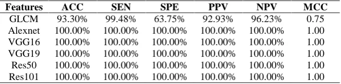
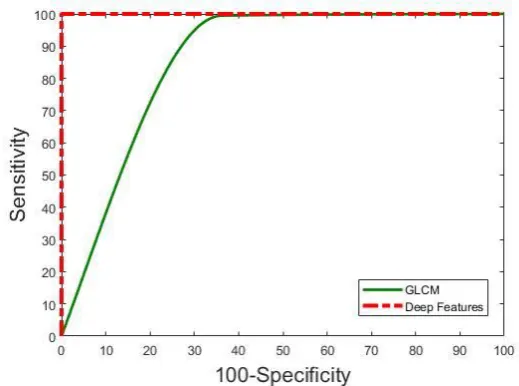
The study then used SVM as the classifier with a 10-fold validation as shown in Table 2. SVM outperformed decision tree when classifying with all the six feature sets. Similarly to decision tree performed the last with accuracy of 93.30%. This was an increase of 11.87% when SVM. All the other performance measures showed a similar trend. An interesting and encouraging observation was that all the deep features achieved the highest performance with the highest accuracy of 100%. Again all the other performance measures concur with the high accuracy. This shows the ability of using deep features for high performance of predicting diseased and normal lungs. The corresponding ROC curves are plotted in Fig. 9. Since the deep learning works performed similarly they are group as one curve (red) which outperformed the GLCM curve (green). It can be seen that the performance of deep features clearly outperform that of the traditional GLCM.

Table. 1 – Classification Performance when using Decision Tree Classifier (10-fold).

Features ACC SEN SPE PPV NPV MCC

GLCM 81.43% 89.56% 42.50% 88.17% 45.95% 0.33

Alexnet 89.20% 93.47% 68.75% 93.47% 68.75% 0.62 VGG16 87.26% 90.34% 72.50% 94.02% 61.05% 0.59 VGG19 89.20% 92.69% 72.50% 94.16% 67.44% 0.63 Res50 96.33% 98.41% 87.06% 97.13% 92.50% 0.88 Res101 89.63% 94.20% 69.05% 93.21% 72.50% 0.64

Table. 2 – Classification Performance when using SVM Classifier (10-fold).

Features ACC SEN SPE PPV NPV MCC

(9)

Fig. 8 – Classification Performance when using Decision Tree Classifier (10-fold).

Fig. 9 – Classification Performance when using SVM Classifier for all deep features and GLCM (10-fold).

Since all five deep feature sets can achieve 100% accuracy with SVM classifier, another important consideration is computational time. This is particularly important for real world applications where there is large data sets and urgency for diagnosis for treatment planning. The computational times of the feature extraction process using the five pre-trained deep learning networks are shown in Table 3. Alexnet showed the lowest computational time at 5.90s. Res50 and Res101 showed considerably more time compared to the rest at 146.62s and 271.85s. VGG16 and VGG19 have a relatively moderate computational time. Since Alexnet has the lowest computational time for feature extraction, the next experiment protocol focuses only on Alexnet.

Table. 3 – Computational Time of Different Deep Learning Architectures.

Features Computational Time of Feature Extraction (s)

Alexnet 5.90

VGG16 22.82

VGG19 27.23

Res50 146.62

(10)

5.2 Classification Performance of Deep Features from Alexnet + PCA

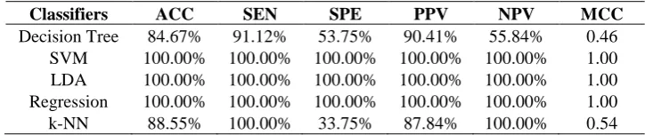
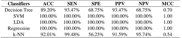
In this subsection, the fastest deep learning network classification performance with and without Principal Component Analysis (PCA) was shown in detail with five different classifiers. The classification performance before PCA implementation for K=2, 3, 5 and 10 folds were shown from Table 4 to Table 7. An immediate and encouraging observation was the high performance of Alexnet when using three classifiers SVM, LDA and Regression for all four folds. This shows the consistency of the algorithm and adds to the stability of using these features when paired with these three classifiers. The significance of this observation was that regardless of the size of training data and testing data, consistent and high classification was able to be achieved using SVM, LDA and regression classifiers. When using Decision Tree and k-NN classifiers, it was noticeable that both perform poorly especially in the specificity measure. This showed that both classifiers classify healthy patients poorly. It can also be seen that k-NN consistently had high sensitivity meaning it can consistently classify diseased patients. However this can be also caused by overfitting where the classifier tends to classify a majority of patients as diseased. This notion was supported by the low specificity. The high NPV value was misleading especially when overfitting of classifying patients as diseased patients caused very low to zero false negative predictions. Therefore MCC is a good indicator of performance here again as seen k-NN produced MCC values from 0.54 to 0.71. Generally there was an increase in performance from K=2 to K=10 validation protocols where the presence of more training data increases the performance of Decision Tree and k-NN.

Table. 4 – Classification Performance for Alexnet with different classifiers before PCA (2-fold).

Classifiers ACC SEN SPE PPV NPV MCC

Decision Tree 84.67% 91.12% 53.75% 90.41% 55.84% 0.46 SVM 100.00% 100.00% 100.00% 100.00% 100.00% 1.00 LDA 100.00% 100.00% 100.00% 100.00% 100.00% 1.00 Regression 100.00% 100.00% 100.00% 100.00% 100.00% 1.00 k-NN 88.55% 100.00% 33.75% 87.84% 100.00% 0.54

Decision Tree 89.70% 95.04% 65.06% 92.62% 73.97% 0.63 SVM 100.00% 100.00% 100.00% 100.00% 100.00% 1.00 LDA 100.00% 100.00% 100.00% 100.00% 100.00% 1.00 Regression 100.00% 100.00% 100.00% 100.00% 100.00% 1.00

k-NN 91.58% 99.74% 52.50% 90.95% 97.67% 0.68

k-NN 92.22% 99.74% 56.25% 91.61% 97.83% 0.71

k-NN 92.01% 99.48% 56.25% 91.59% 95.74% 0.70

(11)

SVM, LDA and regression was maintained. When using Decision Tree the accuracy increases from before PCA to after PCA. An example of this is at 2-fold validation in Table 4 and Table 8, the accuracy increased 84.67% to 86.83%. MCC values also increased from 0.46 to 0.52. When increasing the k-fold validation form 2 to 10, the MCC value also increased from 0.52 to 0.74. k-NN with PCA performed inconsistently and relatively poorly compared to before PCA application when comparing MCC values. This can be seen in Table 7 and Table 11, the MCC value drops from 0.70 to 0.54. This can be caused because the principal components chosen had a negative effect in how k-NN works in predicting the classes. k-NN usually performs better with a larger data set where its classification performance depends on choosing the optimal number of neighbors (k), which is different from one data sample to another (Colas & others, 2009; Hassanat, Abbadi, Altarawneh, & Alhasanat, 2014). This weak indication and drop of performance inspired us to look for an optimal number of features that can produce the best results shown in the next sub-section.

Table. 8 – Classification Performance for Alexnet with different classifiers after PCA (2-fold).

k-NN 86.61% 99.74% 23.75% 86.23% 95.00% 0.44

k-NN 87.90% 99.74% 31.25% 87.41% 96.15% 0.51

k-NN 92.22% 99.74% 56.25% 91.61% 97.83% 0.55

k-NN 92.01% 99.48% 56.25% 91.59% 95.74% 0.54

5.3 Effect of No. Principal Components on Accuracy

(12)

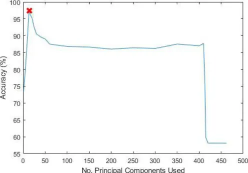
components the results produced are less satisfactory at 92.01%. The accuracy increases steeply at the start until 14 principal components are used. The accuracy started to drop and taper mostly from 40 to 400 principal components. This can be seen as an indication that these principal components do not add any classification value to the k-NN classifier. The addition of more features when passing this threshold had adverse effects on the classification potential as seen by the great decrease of classification accuracy to 58% and ends with this low value. Thus feature selection is important to increase the performance as it minimizes the tendency of generalization of the classifier (Weston et al., 2001). This was suggested in the higher performance achieved.

6. Discussion

This has proposed a lung disease classification system with the use of different deep learning networks and compared it with conventional textural method which was GLCM. Deep learning networks outperformed GLCM reaching a classification accuracy of 96.33% as compared to 81.43% as seen in Table 1 when using Decision Tree. When using SVM classifier, the high performance is clearly seen when all the networks achieved 100% (Table 2) whereas the usage of GLCM produced an accuracy of 93.30%. This suggests to us that deep features can produce very high classification performance. This is a positive observation that it can be applied to even more diverse data of varying background and disease as well. The potential of deep features can be attributed to the convolution network where an image in its raw form is convoluted to show different aspects of it. The CNN used automatically discovers the representations needed to make a proper decision of classification. Textural methods show the relation between pixels and in certain directions. For the deep features used, each feature represents an aspect of the entirety of the image. Thus it is more robust and offer more features in this study case was 1000 features.

The main issue in using deep features has always been the computational power and time and required. For this study, experiments were carried out with a PC powered by an Intel Zeon 3.5GHz processor, memory of 16GB ram and NVIDIA Quadro K2200 graphic card. It is encouraging that when processing 96 patients with five images for each patient, the system only required a minimum of 5.90s for feature extraction (Table 3) when using Alexnet. The fast speed is the benefit of using the method of transfer learning by using a pre-existing and pre-trained network. When compared to training the network from scratch the difference is more prominent. When using the current top performing GPU, NVIDIA 1080 TI, the speed of training Alexnet for just 16 images was 13.89ms (Johnson, 2017). Thus our results using a relatively inferior graphic card and relatively more images was achieved with a comparable time. This is the huge benefit of using pre-trained networks as a form of features and gives a very promising classification performance.

The PCA analysis also shows the ideal number of features used which in this study’s case was 14 features only instead of 1000 features as shown in Fig. 10. When using less features, naturally the computational strain of space and time will be greatly reduced. In this study’s case since the number of features had a reduction of 98.6%, the training and testing time using the SVM classifier also greatly decreased.

Fig. 10 – Classification accuracy when No. Principal Components are varied using k-NN classifier (10-fold).

A concern arises that there might be unfair comparison between GLCM and deep features since GLCM is a rudimentary form of texture and there are far more extensive features such as Gabor transform and Riesz Transform that offer scalability and directional properties for better classification (Depeursinge & Rodriguez, 2011; Kyrki, Kamarainen, & Kälviäinen, 2004). A previous study has shown the performance of 97.52 and 98.97 for Gabor Transform and Riesz Transform respectively when using SVM classifier and the same dataset (Than et al., 2017). Thus this gives us an indication that deep features does outperform even extensive textural features.

(13)

network. Secondly this study highlights the importance of selecting the ideal number of principal components and that using the 95% variation limit might not always be beneficial to achieve the best classification performance

A disadvantage of this study is that it uses an imbalanced ratio of diseased and normal patients. However this is a more realistic representation of the real world where imaging is expensive and healthy people do not typically get a lung thorax CT scan. A person experiencing lung disease symptoms are more inclined to take these scans. However this study uses MCC as a performance measure that can give a holistic view of the performance especially when there is class imbalance. Besides that we also show different performance measures to highlight certain aspects of the classification performance. Also to help overcome this disadvantage we show here a previous work that deals with a balanced class of eight diseased and eight normal patients, the accuracy was still 100% and MCC value was 1.0 when using the SVM classifier.

7. Conclusion

As a conclusion, this study has shown a lung classification framework using deep features for lung disease detection. The usage of deep features help offer a new perspective of feature information from an image as opposed to the conventional texture methods such as GLCM. Using deep features a maximum performance of 96.33% was achieved when using decision tree and 100% when using SVM classifier. The performance increased from 92.01% to 97.40% when using PCA and k-NN classifier. This study has shown that the application of deep features offer a rich and robust feature avenue for predicting diseased and normal lungs. The deep features used has shown its potential that rivals and in some applications outperform GLCM. In the future, the study would like to focus on more feature selection and transform methods to further reduce the number of features required to achieve the best performance. Besides that, we would like to investigate the possibility of using deep features to classify the severity of disease which offer beneficial information for immediate treatment planning.

Acknowledgement

This study is supported under the Research University Grant of Universiti Teknologi Malaysia (Q.K130000 .2540. 14H22) and Ministry of Higher Education Malaysia.

References

[1] Lung, N. H., Institute, B., & others. (2012). Disease statistics. NHLBI Fact Book, Fiscal Year 2012, 35. [2] Malaysia: Lung Disease. In World Health Rankings. (2012). Retrieved from

http://www.worldlifeexpectancy.com/malaysia-lung-disease

[3] Jiang, Y., Nishikawa, R. M., Schmidt, R. A., Metz, C. E., Giger, M. L., & Doi, K. (1999). Improving breast cancer diagnosis with computer-aided diagnosis. Academic Radiology, 6, 22–33.

[4] Doi, K. (2007). Computer-aided diagnosis in medical imaging: Historical review, current status and future potential. Computerized Medical Imaging and Graphics, 31, 198–211.

[5] Shrivastava, V. K., Londhe, N. D., Sonawane, R. S., & Suri, J. S. (2016). Computer-Aided Diagnosis of Psoriasis Skin Images with HOS, Texture and Color Features: A First Comparative Study of Its Kind. Computer Methods and Programs in Biomedicine, 126, 98–108.

[6] Cirujeda, P., Cid, Y. D., Müller, H., Rubin, D., Aguilera, T. A., Loo, B. W., … Depeursinge, A. (2016). A 3-D Riesz-Covariance Texture Model for Prediction of Nodule Recurrence in Lung CT. IEEE Transactions on Medical Imaging, 35, 2620–2630.

[7] A Han, F., A Wang, H., A Zhang, G., A Han, H., A Song, B., A Li, L., … A Liang, Z. (2014). Texture Feature Analysis for Computer-Aided Diagnosis on Pulmonary Nodules. Journal of Digital Imaging.

[8] Haralick, R. M., Shanmugam, K., & Dinstein, I. H. (1973). Textural features for image classification. Systems, Man and Cybernetics, IEEE Transactions on, 610–621.

[9] Huber, M. B., Nagarajan, M., Leinsinger, G., Ray, L. a., & Wismuller, a. (2010). Classification of interstitial lung disease patterns with topological texture features. Proceedings SPIE Medical Imaging 2010, 7624, 2–9. [10] Wang, J., Li, F., & Li, Q. (2009). Automated segmentation of lungs with severe interstitial lung disease in CT.

Medical Physics, 36, 4592.

[11] Than, J. C. M. M., Saba, L., Noor, N. M., Rijal, O. M., Kassim, R. M., Yunus, A., … Suri, J. S. (2017). Lung disease stratification using amalgamation of Riesz and Gabor transforms in machine learning framework.

Computers in Biology and Medicine, 89, 197–211.

[12] Mitani, Y., Hirayama, H., Yasuda, H., Kido, S., Hamamoto, Y., Ueda, K., & Matsunaga, N. (2000). A Gabor filter-based classification for diffuse lung opacities in thin-section computed tomography images. In Knowledge-Based Intelligent Engineering Systems and Allied Technologies, 2000. Proceedings. Fourth International Conference on (Vol. 2, pp. 780–783).

(14)

290.

[14] See, Y. C., Noor, N. M., Low, J. L., & Liew, E. (2017). Investigation of face recognition using Gabor filter with random forest as learning framework. In IEEE Region 10 Annual International Conference,

Proceedings/TENCON (Vol. 2017–Decem). doi:10.1109/TENCON.2017.8228031

[15] Annanurov, B., & Noor, N. M. (2017). Feature selection for Khmer handwritten text recognition. In Proceedings of the 2017 IEEE Russia Section Young Researchers in Electrical and Electronic Engineering Conference, ElConRus 2017. doi:10.1109/EIConRus.2017.7910634

[16] Depeursinge, A., & Rodriguez, A. F. (2011). Lung Texture Classification Using Locally – Oriented Riesz Components. Components, 231–238..

[17] Cirujeda, P., Müller, H., Rubin, D., Aguilera, T. A., Loo, B. W., Diehn, M., … Depeursinge, A. (2015). 3D Riesz-wavelet based Covariance descriptors for texture classification of lung nodule tissue in CT. In Engineering in Medicine and Biology Society (EMBC), 2015 37th Annual International Conference of the IEEE (pp. 7909– 7912).

[18] LeCun, Y., Bengio, Y., & Hinton, G. (2015). Deep learning. Nature, 521, 436.

[19] Kazerooni, E. A., Martinez, F. J., Flint, A., Jamadar, D. A., Gross, B. H., Spizarny, D. L., … Lynch 3rd, J. P. (1997). Thin-section CT obtained at 10-mm increments versus limited three-level thin-section CT for idiopathic pulmonary fibrosis: correlation with pathologic scoring. AJR. American Journal of Roentgenology, 169, 977–983. [20] Chia, J., Than, M., Noor, N. M., Rijal, O. M., Yunus, A., & Kassim, R. M. (2014). Lung segmentation for HRCT

thorax images using radon transform and accumulating pixel width. In Region 10 Symposium, 2014 IEEE (pp. 157–161).

[21] Noor, N. M., Rijal, O. M., Than, J., Ming, C., Roseli, F. A., Ming, J. T. C., … Yunus, A. (2013). Segmentation of the Lung Anatomy for High Resolution Computed Tomography (HRCT) Thorax Images. In Advances in Visual Informatics (pp. 165–175). Springer.

[22] Noor, N. M., Than, J. C. M., Rijal, O. M., Kassim, R. M., Yunus, A., Zeki, A. A., … Suri, S. J. (2015).

Automatic Lung Segmentation Using Control Feedback System: Morphology and Texture Paradigm. Journal of Medical Systems, 1.

[23] Otsu, N. (1979). A Threshold Selection Method from Gray-Level Histograms. Systems, Man and Cybernetics, IEEE Transactions on, 9, 62–66.

[24] Ming, J. T. C., Rijal, O. M., Kassim, R. M., Yunus, A., & Noor, N. M. (2016). Texture-based classification for reticular pattern and ground glass opacity in high resolution computed tomography Thorax images. In Biomedical Engineering and Sciences (IECBES), 2016 IEEE EMBS Conference on (pp. 230–234).

[25] Awais, M., Muller, H., & Meriaudeau, F. (2017). Classification of SD-OCT images using Deep learning approach. In 2017 IEEE International Conference on Signal and Image Processing Applications (ICSIPA) (pp. 3–6).

[26] Hooda, R., Sofat, S., Kaur, S., Mittal, A., & Meriaudeau, F. (2017). Deep-learning: A potential method for tuberculosis detection using chest radiography. In 2017 IEEE International Conference on Signal and Image Processing Applications (ICSIPA) (pp. 497–502).

[27] Prasad, S. (2017). Medicinal Plant Leaf Information Extraction Using Deep Features. In 2017 IEEE Region 10 Conference (TENCON) (pp. 2722–2726).

[28] Krizhevsky, A., Sutskever, I., & Hinton, G. E. (2012). ImageNet Classification with Deep Convolutional Neural Networks. Advances In Neural Information Processing Systems, 1–9.

[29] Simonyan, K., & Zisserman, A. (2014). Very deep convolutional networks for large-scale image recognition.

arXiv Preprint arXiv:1409.1556.

[30] He, K., Zhang, X., Ren, S., & Sun, J. (2016). Deep residual learning for image recognition. In Proceedings of the IEEE conference on computer vision and pattern recognition (pp. 770–778).

[31] Wold, S., Esbensen, K., & Geladi, P. (1987). Principal component analysis. Chemometrics and Intelligent Laboratory Systems, 2, 37–52.

[32] Jolliffe, I. (2011). Principal component analysis. In International encyclopedia of statistical science (pp. 1094– 1096). Springer.

[33] Colas, F. P. R., & others. (2009). Data mining scenarios for the discovery of subtypes and the comparison of algorithms. Leiden Institute of Advanced Computer Science (LIACS), Faculty of Science, Leiden University. [34] Hassanat, A. B., Abbadi, M. A., Altarawneh, G. A., & Alhasanat, A. A. (2014). Solving the problem of the K

parameter in the KNN classifier using an ensemble learning approach. arXiv Preprint arXiv:1409.0919. [35] Weston, J., Mukherjee, S., Chapelle, O., Pontil, M., Poggio, T., & Vapnik, V. (2001). Feature selection for

SVMs. In Advances in neural information processing systems (pp. 668–674).

[36] Johnson, J. (2017). Benchmarks for popular CNN models. Retrieved July 13, 2018, from https://github.com/jcjohnson/cnn-benchmarks