URBAN SPRAWL SHAPE DESCRIPTION

(1)

Malaysian Journal of Computing Vol. 2, Issue 1, 2014

ISSN 2231-7473

URBAN SPRAWL SHAPE DESCRIPTION

N. Laila A. Ghani

1

, Siti Z.Z. Abidin

2

and N. Elaiza A. Khalid

3 Faculty of Computer and Mathematical Sciences,

University Technology MARA, 40450, Shah Alam, Selangor

MALAYSIA

1_{[email protected],}2_{[email protected],}3_{[email protected]}

Abstract

Urban sprawl is the out-of-control growth of urban area as a result of improper urbanization plan. Literatures have characterized various forms of urban sprawl that includes low-density and leapfrog sprawl. The forms of sprawl can be modelled via satellite remote sensing images.This research is mainly about classifying the forms of urban sprawl by using pixel-based approach and representing the sprawl shape using centroid distance Fourier descriptor. The datasets are in the form of Landsat Thematic Mapper(TM) images of Klang Valley, Malaysia,at spatial resolution of 30 meters where each pixel in the image represents the area of 900 square meters on the ground. Results obtained show that the Fourier descriptor graph representation of low-density sprawl is denser than leapfrog sprawl. Due to the rapid urbanization process in Malaysia, it is important to identify the sprawling pattern for a better decision making in planning potential land area to be developed.

Keywords: Urban sprawl, Remote sensing, Shape description, Fourier descriptor

1. Introduction

In the context of land-use, the term ‘sprawl’ was introduced by Earle Draper, who is among the first city planners in the United States (Necyba & Walsh 2004). He referred sprawl as an unattractive and uneconomic form of city expansion. Since then, planners have been using the term to describe undesired urban growth.

Few literatures have defined sprawl based on the forms of urban growth. Ewing (1997), Carruthers & Ulfarsson (2002) and Burchell & Galley (2003) had identified that there are multiple forms of urban growth. Three forms of urban growth most often characterized as sprawl are low-density, ribbon and leapfrog development.

Low-density sprawl is the development that takes place alongside the boundaries of existing urban areas. Dissimilar to low-density sprawl, a ribbon sprawl occurs along the major transportation network that connects the urban areas. In other words, lands around the network are developed but those without direct access to the network remains rural or undeveloped. On the contrary, a leapfrog sprawl is a discontinuous pattern of urbanization in which the developed areas are widely scattered from each other (Ab Ghani et al., 2011).

(2)

28

Since there are limited information on the characteristics of urban sprawl especially in developing countries (Bhatta, 2010), this research aims to determine the distinctive criteria of each urban sprawl form and propose suitable shape description technique for urban sprawl. The proposed technique will be tested in a testing engine developed in image processing software.

The study area is the region of Klang Valley or Lembah Klang, which is one of the most rapid urban growth areas in Malaysia. The covering land area is Latitude 2° 54’ south to latitude 3° 10’ south and longitude 100° 30’ east to longitude 101° 47’ which is equal to 900 km2

(30 km x 30 km). It comprises of Kuala Lumpur, Rawang, Selayang, Gombak, Ampang, Petaling Jaya, Subang Jaya, Shah Alam, Klang, Serdang, Kajang, Puchong, Putrayaja and Cyberjaya.

2. Related Works

A. Urban Sprawl

Industrial Revolution that started off in 18th century has made significant changes to the countries around the world including Malaysia. Historically, Malaysia has experienced a rapid urbanization growth due to the industrialization and related residential growth (Samat, 2007). In order to accommodate the rapid increase of urban population, the boundary of the city expanded and in most cases becoming sprawl. Urban sprawl refers to the unplanned, uncontrolled and uncoordinated development of urban areas occurring along highways, margins of cities and roads connecting a city.

Previous section has described three forms of urban sprawl: low-density, ribbon and leapfrog development. Angel et al. (2007) also classified three forms of sprawl: secondary urban center, ribbon development and scattered development. Based on the literatures, there are many different terms used to describe the similar urban sprawl forms. Hence, in this paper, the terms low-density, ribbon and leapfrog development will be used. These three urban sprawl forms are exclusive of each other, meaning that a developed area can be part of low-density or ribbon development or leapfrog development, but not all three.

Angel et al. (2007) defined the unique criteria of each type of urban sprawl pattern. The development of an urban area usually consists of the main urban core, low-density, regular, ribbon and leapfrog development. Main urban core is the largest continuous group of developed areas with at least 50 percent of its surrounding neighborhood is developed. Low-density development is defined as the developed area with neighboring areas of at least 50 percent developed. Regular development is the developed areas with neighboring areas between 30 to 50 percent developed. Ribbon development is defined as semi-continuous strands of developed areas that are less than 100 meters wide with neighboring areas of less than 30 percent developed. Leapfrog development is defined as the developed areas with neighboring areas of less than 30 percent developed. The neighboring areas covers the area of 1 kilometer2 surrounding each developed area.

B. Shape Description Techniques

Shape description is characterized by extracting shape’s information using shape description approaches. It generates a shape descriptor vector or feature vector from a given shape (Loncaric, 1998).

According to Yang et al. (2008), the required properties of an efficient shape description method are:

 Different shapes have unique features differentiating them from one another;

 Translation, rotation, scale, affine and occultation transformation does not affect extracted features;

(3)

29

 Two different features must be statistically independent;

 Extracted features remain the same, as long as it is the same pattern.

Zhang and Lu (2004) generally classified the techniques into contour-based and region-based approaches. Contour-region-based approach only extracts information about shape boundary to obtain shape representation. The techniques include chain code, polygon, shape signature, wavelet descriptors, elastic matching and simple shape descriptors like perimeter, compactness and eccentricity. On the other hand, region-based approach takes into account all the pixels within a shape region to obtain the shape representation. The examples of techniques include geometric moments, Zernike moments, Fourier descriptor, grid method, convex hull and simple shape descriptors like area and Euler number.

Region-based approach is more robust and accurate as compared to contour-based approach that is sensitive to noise and variations. Zhang and Lu (2004) concluded that shape representation using Fourier descriptor, either one-dimensional or two-dimensional, is simple to compute, robust and compact. It overcomes the weakness of simple shape descriptors, noise sensitivity and normalization difficulty in shape signature representation.

3. Methodology

A. Data Collection

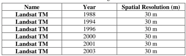
Data used in this research is collected from the Department of Survey and Mapping Malaysia. Six Landsat Thematic Mapper (TM) images at spatial resolution of 30 meters are used where each pixel in the image represents the area of 900 square meters on the ground. All images represent the study area for the year 1988, 1994, 1996, 2000, 2001 and 2003. The summarized details on the satellite image datasets are shown in Table 1.

Table. 1. Satellite images datasets

Name Year Spatial Resolution (m)

Landsat TM 1988 30 m

B. Data Pre-processing

a. Classification of developed and undeveloped area using ENVI software

(4)

30

Figure. 1. Sample dataset of satellite image viewed in ENVI.

The resulting image is saved in binary format representing only developed and undeveloped cells. Each image is in the form of bitmap image with the size of 827 pixels width and 467 pixels height, containing 383728 (827 x 467) data of both developed and undeveloped areas. Each pixel represents a ground area of 900 square meters (30 meters x 30 meters). The developed area is denoted as white colour with pixel value 1 while black colour represents the undeveloped area with pixel value 0.

b. Image Correction

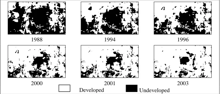
Image correction procedure is performed to the binary images obtained from ENVI by checking for any classification error in the images. Classification error in this case means areas that are already developed in preceding year are found to be undeveloped in succeeding year. The procedure compares two binary images discrepancies between developed pixel (1) in the first image and undeveloped pixel (0) in the second image. The discrepancies are then corrected in the second image. Figure 2 shows all corrected outputs that will be used to classify the forms of urban sprawl.

1988 1994 1996

2000 2001 2003

Figure. 2. Actual datasets for urban sprawl classification.

C. Sprawl Classification

For each dataset, a circle-shaped moving window with radius of 19 that is equals to 1 kilometer2 area, is created. The moving window is centred on each developed pixel to determine the number of developed pixels in the neighbourhood and the percentage of developed pixels over the total number of neighbourhood is then calculated. If the neighbourhood percentage is more than or equal to 50 percent and the pixel belongs to largest continuous group of pixels, then the pixel is assigned in the main urban core group. Otherwise, if the pixel does not belong to the main urban core with neighbourhood percentage of more than or equal to 50 percent, it is assigned in the low-density sprawl group. If the neighbourhood percentage is between 30 to 50 percent, the pixel is assigned in the regular urban development group. If the neighbourhood percentage is less than 30

Developed land Undeveloped land

(5)

31

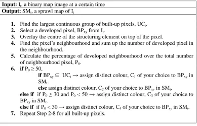
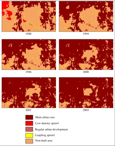
percent, it is assigned as leapfrog sprawl group. A sprawl forms map consisting of the main urban core, low-density sprawl, leapfrog sprawl and regular urban development will be produced. Note that ribbon sprawl will not be examined in this research due to the absent of road factor during pre-processing of the datasets. Figure 3 shows the general pseudocode involved in producing the sprawl map.

Input: It, a binary map image at a certain time Output: SMt, a sprawl map of It

1. Find the largest continuous group of built-up pixels, UCt. 2. Select a developed pixel, BPxy from It.

3. Overlay the centre of the structuring element on top of the pixel.

4. Find the pixel’s neighbourhood and sum up the number of developed pixel in

the neighbourhood.

5. Calculate the percentage of developed neighbourhood over the total number of neighbourhood pixel, P0.

6. if P0 ≥ 50,

if BPxy⊆ UCt → assign distinct colour, C1 of your choice to BPxy in

SMt.

else assign distinct colour, C2 of your choice to BPxy in SMt.

else if if P0 ≥ 30 and P0 < 50 → assign distinct colour, C3 of your choice to

BPxy in SMt.

else if if P0 < 30 → assign distinct colour, C4 of your choice to BPxy in SMt. 7. Repeat Step 2-8 for all built-up pixels.

Figure. 3. General pseudocode of producing the sprawl forms map.

D. Sprawl Shape Representation

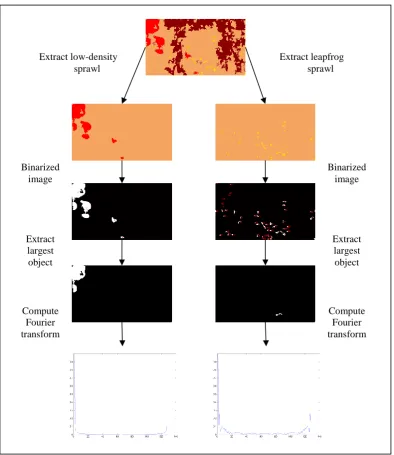
Two separate images of low-density sprawl and leapfrog sprawl are extracted from the sprawl form map of each dataset. Then, for each image, the largest object from is extracted as the focus of this research is only to get the Fourier descriptor of the largest sprawl areas. Each boundary points and the centroid of the object are traced in order to calculate the centroid distance function of each boundary points. The Fourier transforms of all centroid distance functions is computed by applying the pseudocode in Figure 4.

Input: Ot, an image containing object of interest Output: FDt, fourier transform of Ot

1. Trace boundary points of the object.

2. Trace centroid of the object.

3. Calculate the centroid distance function of each boundary points:

√( ) ( )

4. Compute Fourier transform of all centroid distance functions.

(6)

32

Figure 5 shows the visual diagram of sprawl shape representation procedure for one dataset as described previously. Each dataset produces one Fourier Descriptor of low-density sprawl and one Fourier Descriptor of leapfrog sprawl.

Figure. 5. Visual diagram of sprawl shape representation procedure.

4. Experimental Results

A. Classification of Urban Sprawl Pattern

Six urban sprawl map of Klang Valley for year 1988, 1994, 1996, 2000 and 2001 are obtained (see Figure 6). Pixels or areas that are coloured in dark red represent the main urban core or the town centre of Klang Valley. Areas coloured in red represent the secondary urban core development or better known as the low-density sprawl, light red

Extract leapfrog sprawl Extract low-density

sprawl

Binarized image Binarized

image

Extract largest object Extract

largest object

Compute Fourier transform Compute

(7)

33

coloured areas signify regular urban development that are not categorized as sprawl while the areas in yellow is the scattered development or leapfrog sprawl.

1988 1994

1996 2000

2001 2003

Figure. 6. Forms of urban sprawl at Klang Valley, Malaysia within 1988 until 2003.

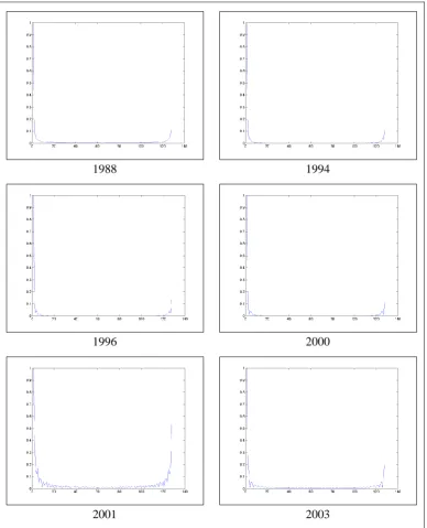
B. Shape Representation of Urban Sprawl using Fourier Descriptor

Six Fourier descriptor graph representation of low-density sprawl are obtained from the largest low-density sprawl region in each sprawl map (see Figure 7).

Main urban core

Low-density sprawl

Regular urban development

Leapfrog sprawl

(8)

34

1988 1994

1996 2000

2001 2003

Figure. 7. Fourier descriptor graph representation of low-density sprawl

(9)

35

1988 1994

1996 2000

2001 2003

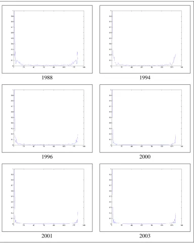
Figure. 8. Fourier descriptor graph representation of leapfrog sprawl

When comparing both shapes, the low-density and leapfrog sprawl, the Fourier descriptor graph representation of the year 1988 to 2000 give the obvious differences due to most areas are still developing according to the map. The graph representation for low-density sprawl is denser than the graph representation for leapfrog sprawl.

5. Conclusion

(10)

36

Since this research only applied Fourier descriptor to represent urban sprawl shape, urban sprawl shape representation using other shape descriptors can be further investigated in the future.

References

Ab Ghani, N. L., Abidin, S. Z., & Abiden, M. Z. Z (2011). Generating Transition Rules of Cellular Automata for Urban Growth Prediction. International Journal of Geology, 5 (2), 41-47.

Angel A., Parent J., & Civco D. (2007). Urban Sprawl Metrics:An Analysis of Global Urban Expansion Using GIS. ASPRS 2007 Annual Conference.

Bhatta B. (2010). Chapter 1 Urban Growth and Sprawl.In B. B., Analysis of Urban Growth and Sprawl from Remote Sensing Data, Advances in Geographic Information Sciences (pp. 1-16). Springer.

Burchell R.W., & Galley C.C. (2003). Projecting Incidence and Costs of Sprawl in the United States. Transportation Research Board of the National Academies, 1831/2003, 150-157.

Carruthers J.I., & Ulfarsson G.F. (2002). Urban Sprawl. Journal of Economic Perspectives ,18

(4), 177-200.

Ewing R. (1997). Is Los Angeles-Style Sprawl Desirable?. Journal of the American Planning Association, 63 (1), 107.

Loncaric S. (1998). A survey of shape analysis techniques. Pattern Recognition, 31(8) , 983-1001.

Nechyba T.J., & Walsh R.P. (2004). Urban Sprawl. Journal of Economic Perspectives, 18 (4), 177-200.

Samat N. (2007). Integrating GIS and CA Spatial Model in Evaluating Urban Growth:Prospect and Challenges. Jurnal Alam Bina, 09 (01).

Sudhira H.S., Ramachandra T.V., & Jagadish K.S. (2003). Urban Sprawl Pattern Recognition and Modeling using GIS. Map India Conference.

Taubenböck H., Esch T. (2011). Remote Sensing – An Effective Data Source for Urban Monitoring. In Earthzine IEEE Magazine.

Retrieved from

http://www.earthzine.org/2011/07/20/remote-sensing-%e2%80%93-an-effective-datasource-for-urban-monitoring/

Yang Mingqiang, Kpalma Kidiyo, Ronsin Joseph (2008). A survey of shape feature extraction techniques. Pattern Recognition, Peng-Yeng Yin (Ed.) 43-90.

Zhang D., & Lu G. (2004). Review of Shape Representation and Description Techniques.