www.theoryofcomputing.org
Dual Polynomials for
Collision and Element Distinctness
Mark Bun
∗Justin Thaler
†Received August 17, 2015; Revised May 8, 2016; Published October 13, 2016
Abstract: The approximate degree of a Boolean function f :{−1,1}n→ {−1,1}is the
minimum degree of a real polynomial that approximates f to within error 1/3 in the`∞ norm. In an influential result, Aaronson and Shi (J. ACM, 2004) proved tightΩe(n1/3)and
e
Ω(n2/3)lower bounds on the approximate degree of the COLLISION and ELEMENTDIS -TINCTNESSfunctions, respectively. Their proof was non-constructive, using a sophisticated symmetrization argument and tools from approximation theory.
More recently, several open problems in the study of approximate degree have been resolved via the construction of dual polynomials. These are explicit dual solutions to an appropriate linear program that captures the approximate degree of any function. We reprove Aaronson and Shi’s results by constructing explicit dual polynomials for the COLLISION
and ELEMENTDISTINCTNESSfunctions. Our constructions are heavily inspired by Kutin’s (Theory of Computing, 2005) refinement and simplification of Aaronson and Shi’s results.
ACM Classification:F.1.2, F.1.3
AMS Classification:68Q12, 68Q17
Key words and phrases:polynomials, polynomial approximation, approximate degree, quantum com-puting, collision problem, element distinctness
∗Harvard University, School of Engineering and Applied Sciences. Supported by an NDSEG Fellowship and NSF grant
CNS-1237235.
†Yahoo Research. Parts of this work were performed while the author was a Research Fellow at the Simons Institute for the
1
Introduction
Theε-approximate degree of a Boolean function f :{−1,1}n→ {−1,1}is the least degree of a real
polynomial that approximates f to within errorε in the`∞norm. Approximate degree is a fundamental measure of the complexity of a Boolean function, and has wide-ranging applications in theoretical computer science. For example, approximate degree upper bounds underlie several of the best known algorithms for PAC learning [26], agnostic learning [24, 25], learning in the presence of irrelevant information [27, 35], and differentially private data release [49, 21]. Meanwhile, lower bounds on approximate degree imply many optimal lower bounds on quantum query complexity, circuit complexity, and communication complexity (see for example [11,37,5,18,45,38,13,12,36]).
In an influential result, Aaronson and Shi proved tightΩe(n1/3)andΩe(n2/3)lower bounds on the approximate degree of the COLLISIONand ELEMENT DISTINCTNESSfunctions [5].1 The COLLISION
lower bound matched an earlierO(n1/3)upper bound due to Brassard et al. [17], while the lower bound for ELEMENTDISTINCTNESSwas later shown to be tight by Ambainis [9].
The COLLISION lower bound subsequently found many applications and extensions in quantum complexity theory; Aaronson recently provided a retrospective overview of these developments [4]. Moreover, theΩe(n2/3)lower bound for ELEMENTDISTINCTNESSremains the best known approximate degree lower bound for any function inAC0.
Aaronson and Shi proved their lower bound for COLLISIONwith a symmetrization argument. This
style of argument proceeds in two steps. First, a polynomial ponnvariables (which is assumed to approximate the target function f) is transformed into a polynomialqon m<nvariables in such a way that deg(q)≤deg(p). Second, a lower bound on deg(q)is proved, typically by applying Markov-Bernstein type inequalities from approximation theory. Aaronson and Shi’s proof of the COLLISION
lower bound is a particularly sophisticated application of this style of argument.
The lower bound for ELEMENT DISTINCTNESSfollows from a reduction to the lower bound for
COLLISION. This reduction is discussed inSection 5.
1.1 The method of dual polynomials
Despite the many applications of approximate degree in theoretical computer science, significant gaps remain in our understanding of this complexity measure, and there are many simple functions whose approximate degree remains unknown. The slow nature of progress can be attributed in part to the limitations of symmetrization arguments. At an intuitive level, the process of symmetrization is inherently lossy: by turning a polynomialponnvariables into a polynomialqonm<nvariables, information about pis necessarily thrown away. Hence, several works have identified that an important research direction is to develop techniques beyond symmetrization for lower bounding the approximate degree of Boolean functions [2,41,19].
The last few years have seen significant progress toward this goal. In particular, a series of works has proved new approximate degree lower bounds for important classes of functions by constructing
1Aaronson established a lower bound of
e
Ω(n1/5)for the COLLISIONfunction in a paper that appeared in STOC 2002 [1], and Shi improved it to the tightΩ(e n1/3)in a FOCS paper that same year [44]. A joint journal paper appeared in 2004 [5]. The
explicitdual polynomials, which are dual solutions to a certain linear program capturing the approximate degree of any function. These polynomials act as certificates of the high approximate degree of a function. Moreover, strong LP duality implies that the technique is lossless, in contrast to symmetrization. That is, for any function f and anyε, there is always some dual polynomialφ that witnesses a tight approximate
degree lower bound for f; the challenge is to constructφ.
This “method of dual polynomials” was recently used to resolve the approximate degree of the AND-OR tree [40,19], closing a long line of incrementally larger lower bounds [44,7,23,41,30]. It has also been used to establish several “hardness amplification” results for approximate degree [48,20,42], and to prove newthreshold degreelower bounds for several important classes of functions, including the intersection of two majorities [31, 41] andAC0 [42, 43]. The latter result represented the first superlogarithmic improvement over Minsky and Papert’s seminalΩ(n1/3)lower bound from 1969 on the threshold degree of anAC0function. We also note that dual polynomials have been used via thepattern matrix method[38] to resolve several longstanding open problems in communication complexity (see the survey of Sherstov [36]). The pattern matrix method uses dual polynomials to construct distributions under which various communication problems are hard (see the next section for more details).
1.2 Contribution and motivation
We reprove Aaronson and Shi’s results by constructing explicit dual polynomials for the COLLISION
and ELEMENT DISTINCTNESSfunctions.2 First, we give a direct construction of a dual polynomial for COLLISION. The construction of this dual polynomial is heavily inspired by Kutin’s refined proof of the COLLISION lower bound [28]. InSection 2.5, we give an overview of the ideas that go into this construction. InSection 5, we give a generic reduction which shows show how to turn any dual polynomialψ for COLLISIONinto a dual polynomialϕ for ELEMENTDISTINCTNESS. We construct
ϕ(x)by averagingψ(y)over a carefully constructed set of extensions from eachxto a longer inputy. We have four main motivations for reproving Aaronson and Shi’s lower bound in this manner.
1. First, only a handful of techniques are currently known for the construction of dual polynomials, especially for the case whereε=Θ(1). To date, dual polynomials have been constructed only for symmetric functions [46,19] and a handful of highly structured block-composed functions [20,
19,40,41,42,43,39]. (Ablock-composedfunctionF:{−1,1}M·N→ {−1,1}is a function of the
form of the formF=g(f(x1), . . . ,f(xM))for someg:{−1,1}M→ {−1,1}and f:{−1,1}N→
{−1,1}.) The COLLISIONand ELEMENTDISTINCTNESSfunctions fall into neither category; our
constructions of dual polynomials for these problems introduce several new techniques that we are optimistic will prove useful in future applications.
In particular, we hope that our techniques will prove useful for establishing new, stronger ap-proximate degree lower bounds for AC0. Up to polylogarithmic factors, the best lower bound on the approximate degree of any function inAC0is theΩe(n2/3)lower bound for the ELEMENT DISTINCTNESSfunction. Meanwhile, noo(n)upper bound is known. Resolving the approximate degree ofAC0remains a significant open problem with many complexity-theoretic applications, and the new techniques that we use to construct dual polynomials may help close the gap.
2Like Kutin’s simplification and refinement of Aaronson and Shi’s original proof of the COLLISIONlower bound, our
2. A second motivation is to shed new light on the COLLISION lower bound itself. The earlier symmetrization-based proof [5, 28], while shorter than ours, is non-constructive and relies on Markov-Bernstein inequalities from approximation theory. In contrast, our proof is constructive and entirely elementary. We also believe that our analysis illuminates some of the more miraculous aspects of the earlier symmetrization-based proof—seeSection 2.6for further discussion of this point.
3. Our third motivation is to make explicit the proofs of several of the best known bounds in the complexity-theoretic study of constant-depth circuits. In particular, very recent work of Sher-stov [43] exhibits a functionFinAC0with threshold degreeΩ(n1/2). The functionFis obtained by block-composing the ELEMENTDISTINCTNESSfunction with a certain constant-depth Boolean formula, and Sherstov’s proof is via the method of dual polynomials. There is only one non-explicit element in Sherstov’s construction of a dual polynomialφ witnessing the fact that the threshold
degree ofF is inΩ(n1/2); he uses, in a black-box manner, theexistenceof a dual polynomial for ELEMENTDISTINCTNESS. In giving the first explicit construction of such a dual polynomial, we
render Sherstov’s construction ofφ fully explicit. This has the following implication.
By applying the pattern matrix method to Sherstov’s function F, one obtains a function Gin
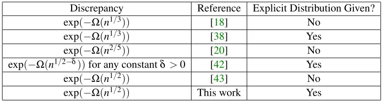
AC0 withdiscrepancyexp(−Ω(n1/2)).3 This is the strongest known bound on the discrepancy of a function in AC0, improving over a lengthy line of work (seeTable 1). However, because the construction of the dual polynomialφ in [43] is not entirely explicit, combining Sherstov’s
result [43] with the pattern matrix method does not give an explicit distribution under whichGhas low discrepancy. Our construction of a dual polynomial for ELEMENTDISTINCTNESSremedies this situation, yielding the first explicit distribution under which anAC0function has discrepancy exp(−Ω(n1/2)).
We remark that several other applications of the method of dual polynomials have utilized the existence of a dual polynomial for ELEMENTDISTINCTNESSin a black-box fashion [42,20]. Our results render explicit these dual polynomial constructions as well.
4. Finally, following the initial dissemination of this work, Bogdanov et al. [16] used our dual polynomial for ELEMENT DISTINCTNESS to design an explicit secret sharing scheme with a reconstruction algorithm computable by anAC0 circuit. An (n,d)-secret sharing scheme with reconstruction advantage ε is a procedure that enables a dealer to share a secret bit between n parties in such a way that any coalition of at most d parties learns nothing about the secret, but the n parties can combine all of their shares to recover a (randomly chosen) secret with probability at least 1/2+ε. Bogdanov et al. [16] showed that if the ε-approximate degree of
a function f :{−1,1}n→ {−1,1}is at least d, then there exists a(n,d)-secret sharing scheme
with reconstruction advantage at leastε/2, in which thenparties apply f to their shares in order to reconstruct the secret bit. Moreover, the distributions from which the dealer samples shares are exactly determined by a dual polynomial for f. Thus, for any constant ε <1, our dual
3Low discrepancy implies high communication cost in nearly every communication model. We refer the reader to [38,
Discrepancy Reference Explicit Distribution Given?
exp(−Ω(n1/3)) [18] No
exp(−Ω(n1/3)) [38] Yes
exp(−Ω(n2/5)) [20] No
exp(−Ω(n1/2−δ))for any constantδ >0 [42] Yes
exp(−Ω(n1/2)) [43] No
exp(−Ω(n1/2)) This work Yes
Table 1: Upper bounds on the discrepancy of circuits of constant depth and polynomial size.
polynomial for ELEMENT DISTINCTNESSyields an explicit(n,Ωe(n2/3))-secret sharing scheme with reconstruction advantage at leastε/2. Bogdanov et al. additionally showed that the structure of our dual polynomial enables these shares to be sampled byAC0circuits.
1.3 Related work on quantum query complexity
Aaronson and Shi’s original motivation for studying the approximate degree of the COLLISIONfunction
was to understand its quantum query complexity. (Recall that approximate degree provides alower boundon quantum query complexity [11]. However, it is known that the lower bound is not always tight [8].) Subsequent to Aaronson and Shi’s work, a body of lower bound techniques collectively known asadversary methodswere developed for quantum query complexity [22,6,47,8,52,10]. It is now known that one of the most general forms of the adversary method, called thenegative-weights adversary method[22], always gives a tight characterization of quantum query complexity [33,34]. (Moreover, the polynomial method can be viewed as a special case of the multiplicative adversary method [29].)
The negative-weights adversary method for lower bounding quantum query complexity is closely analogous to the method of dual polynomials for approximate degree; the former is characterized by a semidefinite program, and a solution to this semidefinite program is known as anadversary matrix. A recent line of work, similar in spirit to our own, has proved or reproved optimal quantum query complexity lower bounds for several functions by constructing explicit adversary matrices. In particular, Belovs and Rosmanis [14] constructed an optimal adversary matrix for the COLLISIONfunction in the “large range” case (note that the dual polynomial that we construct applies even in the “small range” case), and Belovs and Špalek constructed an optimal adversary matrix for the ELEMENTDISTINCTNESSfunction [15].
Very recently, Zhandry [51] (improving on work of Yuen [50]) proved a tight lower bound ofΩ(N1/3)
on the quantum query complexity of finding a collision in a randomly chosen function.
2
Preliminaries
2.1 Notation
For any positive integern, we denote the set{1, . . . ,n}by[n], and the set{0,1, . . . ,n}by[[n]]. For a function f:D→R, define theL1normkfk1=∑x∈D|f(x)|. For any subsetS⊆[n], we letχS:{−1,1}n→
2.2 Approximate degree and its dual characterization
LetD⊆ {−1,1}n, and let f:D→ {−1,1}be a partial Boolean function defined onD. A real polynomial p:{−1,1}n→
Ris said toε-approximate f if
1. |p(x)−f(x)| ≤εfor allx∈D, and
2. |p(x)| ≤1+ε for allx∈ {−1,1}n.
Theε-approximate degree of f, denoteddegfε(f), is the minimum degree of anε-approximation for
f. We usedegf(f)to denotedegf1/3(f), and refer to this quantity without qualification as theapproximate
degreeof f. The choice of 1/3 is arbitrary, asdegf(f)is related todegfε(f)by a constant multiplicative factor for any constantε∈(0,1).
Given a partial Boolean function f, letpbe a real polynomial that attains the smallestε subject to the
constraints above, over all polynomials of degree at mostd. Since we work overx∈ {−1,1}n, we may
assume without loss of generality thatpis multilinear with the representation
p(x) =
∑
|S|≤dcSχS(x),
where the coefficientscSare real numbers. Then pis an optimum of the following linear program.
min ε
such that
f(x)−∑|S|≤dcSχS(x)
≤ε for eachx∈D
∑|S|≤dcSχS(x)
≤1+ε for eachx∈ {−1,1}
n\D
cS∈R for each|S| ≤d
ε≥0
The dual linear program is as follows.
max ∑x∈Dφ(x)f(x)−∑x∈{−1,1}n\D|φ(x)|
such that ∑x∈{−1,1}n|φ(x)|=1
∑x∈{−1,1}nφ(x)χS(x) =0 for each|S| ≤d φ(x)∈R for eachx∈ {−1,1}n
Strong LP-duality thus implies the following dual characterization of approximate degree.
Theorem 2.1. Let f :D→ {−1,1}be a partial Boolean function. Thendegfε(f)>d if and only if there
is a polynomialφ:{−1,1}n→
Rsuch that
∑
x∈D
f(x)φ(x)−
∑
x∈{−1,1}n\D|φ(x)|>ε·
∑
x∈{−1,1}n|φ(x)|, (2.1)
and
∑
x∈{−1,1}n
Ifφ satisfies (2.1), we say thatφhascorrelation greater thanεwith f. Ifφ satisfies (2.2), i. e., all
Fourier coefficients ofφ below degreed are zero, we sayφ has pure high degree d. We refer to any feasible solutionφ to the dual linear program as an(ε,d)-dual polynomialfor f.
2.3 The COLLISIONand ELEMENTDISTINCTNESSfunctions
Let[N] ={1, . . . ,N}, and fix a triple of positive integersn,N,Rsuch thatR≥N, andn=N·log2R. For simplicity throughout, we assume thatRis a power of 2. The COLLISIONand ELEMENTDISTINCTNESS
functions are typically thought of aspropertiesof functions mapping [N]to[R]. However, it will be convenient for us to think of them instead as functions on the Boolean hypercube{−1,1}n. To this end,
given an inputx∈ {−1,1}n, we interpretxas the evaluations of a functiongxmapping[N]→[R]. That is,
we breakxup intoNblocks, each of length log2R, and regard each blockxias the binary representation
ofgx(i).
Definition 2.2(COLLISIONFunction). A functiongx:[N]→[R]is said to bek-to-1 if for everyi∈[N], there exist exactlyk−1 values j6=isuch thatgx(i) =gx(j). Let Tk :={x∈ {−1,1}n:gxisk-to-1}
(clearly,Tk is non-empty only ifk|N). The COLLISION function, which we denote by ColN,R, is the
partial Boolean function defined onT1∪T2⊆ {−1,1}nsuch that ColN,R(x) =1 if and only ifx∈T1. That
is, ColN,Ris the partial Boolean function corresponding to the property thatgxis a 1-to-1 function, with
the promise thatgxis either 1-to-1 or 2-to-1.
Definition 2.3(ELEMENTDISTINCTNESSFunction). The ELEMENTDISTINCTNESSfunction, denoted EDN,R, is the total Boolean function defined such that EDN,R(x) =1 if and only ifgxis 1-to-1. That is,
EDN,Ris the total Boolean function corresponding to the property thatgxis 1-to-1.
Let B⊂ {−1,1}n denote the set of inputs x such thatgx is neither 1-to-1 nor 2-to-1. Then an
(ε,d)-dual polynomialφfor ColN,Rhas the following properties (cf.Section 2.2):
1. ∑x∈T1φ(x)−∑x∈T2φ(x)−∑x∈B|φ(x)|>ε·∑x∈{−1,1}n|φ(x)|.
2. ∑x∈{−1,1}nφ(x)χS(x) =0 for all|S| ≤d.
Similarly, an(ε,d)-dual polynomial for EDN,Rsatisfies the following conditions.
1. ∑x∈T1φ(x)−∑x∈/T1φ(x)>ε·∑x∈{−1,1}n|φ(x)|.
2. ∑x∈{−1,1}nφ(x)χS(x) =0 for all|S| ≤d.
2.4 Overview of the symmetrization-based proof of the COLLISION lower bound
Kutin’s simplified proof of the COLLISIONlower bound [28] proceeds in two steps. The first step is a symmetrization step, which establishes the following remarkable result. (We state this result slightly informally in this overview.)
Let p(x)be a real polynomial over{−1,1}nof degree d. Then there is a trivariate polynomial P of total degree at most d such that for every valid triple(m,a,b), it holds that
P(m,a,b) =Ex∈Rm,a,b[p(x)].
Note in the above lemma that the setsRm,a,b are not uniquely determined; for instanceRm,1,1= R0,a,1=RN,1,b=T1for every triple(m,a,b).
The second step of Kutin’s proof argues that if p is a(1/3)-approximating polynomial for the COLLISION function, thenPmust have degreeΩ(N1/3). Hence byLemma 2.4, pmust have degree Ω(N1/3)as well.
In more detail, the second step of Kutin’s proof proceeds via a case analysis. Four cases are considered.
Case 1: P(N/2,1,2)≥1/2, and|P(N/2,1,b)| ≤2 for allb∈[N2/3]. In this case, Kutin is able to apply Markov’s inequality from approximation theory to conclude that the degree ofPin its third variable isΩ(N1/3).
Case 2: P(N/2,1,2)≥1/2, and|P(N/2,1,b)|>2 for someb∈[N2/3]. In this case, Kutin is able to apply Bernstein’s inequality from approximation theory to conclude that the degree ofPin its first variable isΩ(N1/3).
Case 3: P(N/2,1,2)<1/2, and|P(N/2,a,2)| ≤2 for alla∈[N2/3]. In this case, Kutin is able to apply Markov’s inequality to conclude that the degree ofPin its second variable isΩ(N1/3).
Case 4: P(N/2,1,2)<1/2, and|P(N/2,a,2)|>2 for somea∈[N2/3]. In this case, Kutin is able to apply Bernstein’s inequality to conclude that the degree ofPin its first variable isΩ(N1/3).
A key technical complication that must be dealt with in the argument above is that|P(m,a,b)|may be much larger than 1 forinvalidtriples(m,a,b). This may seem like a minor technicality, but in fact it is a central issue: ifP(m,a,b)were bounded for all invalid triples, then it would be possible to argue that the total degree ofPisΩ(N1/2), which would imply a (false) lower bound ofΩ(N1/2)on the approximate degree of ColN,R.
2.5 Overview of our construction for the COLLISIONfunction
As with Kutin’s proof, our construction also makes essential use ofLemma 2.4. Whereas Kutin used
Lemma 2.4 to reduce to a setting where Markov-Bernstein inequalities could be applied in a non-constructive manner, we instead useLemma 2.4to argue that the dual polynomialφ that we construct has
pure high degreeΩ(N1/3).
In more detail, we present our construction in two stages, in order to highlight distinct ideas that go into the proof. In the first stage, we construct a simpler dual polynomialφ:{−1,1}n→ {−1,1}that
exhibits anΩ(plogN/log logN)lower bound on the approximate degree of ColN,R. The second stage
Overview of the first stage. LetHk⊆ {−1,1}ndenote the set of inputs of Hamming weightk. The
symmetrization-based proof of the COLLISIONlower bound from [5,28] carries the strong intuition that
the setsTk should play the same role thatHkplays in Nisan and Szegedy’s seminal symmetrization-based lower bound for the OR function [30]. We direct the interested reader to Aaronson’s lecture notes [3] for a detailed explanation of this intuition. The construction of our simpler dual witnessφinstantiates this
intuition in the dual setting.
Recall that a dual polynomialφ witnessing the fact thatdegf(ColN,R)≥dmust satisfy two properties: (1) it must have correlation greater thanεwith ColN,R, and (2) it must have pure high degree at leastd. We
defineφ in a way that mimics the structure of known dual witnesses for symmetric functions, even though φis not itself symmetric. Specifically, our construction ensures that the analysis establishing Properties
(1) and (2) becomes similar to the analyses of known dual polynomials for the OR function [46,19]. In more detail, our prior work [19] built on work of Špalek [46] to give a dual witnessγ for the fact
thatdegfε(ORn) =Ω( √
n)for any constantε <1; moreover,γ places non-zero weight only on setsHk,
for values ofkequal (up to scaling factors) to perfect squares. The pure high degree ofγ is shown to be
equal to (at least) the number of setsHkupon whichγplaces non-zero weight.
Call an inputx∈ {−1,1}nvalidif it is inR
m,a,bfor some valid triple(m,a,b). By analogy withγ,
the dual witnessφ that we construct in Stage 1 places weight only on inputsx∈Tkfor divisorskofN
that are also (up to scaling factors) perfect squares. In particular, our definition ofφensures that
φ(x) =0 for all invalid inputsx. (2.3)
We are able to combine (2.3) withLemma 2.4and a basic combinatorial identity (cf.Lemma 3.2) to show that the pure high degree ofφis at least|S|, whereSdenotes the set ofTk’s upon whichφ places
non-zero weight. In more detail, given any polynomialpof degree at most|S|,Lemma 2.4gives us a measure of control over p’s value on valid inputs. Lemma 2.4providesnocontrol over p’s value on invalid inputs, but this is rendered irrelevant by (2.3), which guarantees thatφ essentially ignores such
inputs.
Moreover, our definition ofφ is carefully chosen to ensure that its correlation with ColN,Ris large;
the precise calculation is closely analogous to the analysis from [46,19] showing thatγis well-correlated
with the OR function [46,19].
Overview of the second stage. In the second stage, we construct a dual polynomialψ that exhibits
the optimalΩ(N1/3)lower bound. Rather than only weighting inputs inTkfor some some divisorskof N,ψ weights inputs inRm,a,bfor many valid triples(m,a,b). There are two key ideas that go into the
construction ofψ.
The first idea is to defineψ as the sum of two simpler dual polynomialsψ1andψ2, each with pure
high degreeΩ(N1/3)—then the sumψ also has pure high degreeΩ(N1/3)(seeLemma 4.5). The first polynomialψ1places a large constant fraction (close to 1/2) of itsL1mass onT1, whereasψ2places a
large constant fraction of itsL1mass onT2. Neitherψ1norψ2is well-correlated with ColN,Rin the sense
of (2.3). However, they each place a constant fraction of theirL1mass onRN/2,2,1, and they are designed
so that their values exactly cancel out on inputs inRN/2,2,1. This allows us to show thatψ=ψ1+ψ2
The second idea goes into the construction ofψ1andψ2themselves. Specifically, we think ofψ1
andψ2as each being constructed in a two-step process. We focus onψ1in this discussion, since the
construction ofψ2is similar. Very roughly speaking, in the first step, we consider a “polynomial”ψ0of
pure high degreeΩ(N1/3)that places a large constant fraction of itsL1mass onT1; the construction ofψ0
is closely related to our construction of the simpler dual polynomialφ from Stage 1.
The reason we place the term “polynomial” in quotes above is that there is an important technical caveat to our construction ofψ0: we think ofψ0as placing weight on setsRN/2,a,1for manyinvalidtriples
(N/2,a,1), in addition to some valid ones. Of course, if(N/2,a,1)is invalid, thenRN/2,a,1= /0, soψ0
cannot place non-zero weight on the set. To address this issue, in Step 2, we add toψ0 a sequence of polynomialsψN00/2,a,1, each of pure high degreeΩ(N1/3). For each invalid triple(N/2,a,1),ψN00/2,a,1is
specifically constructed to cancel out the weight thatψ0“places” onRN/2,a,1.
Analogously to how our constructions ofφ andψ0were closely related to the dual witness for OR
constructed in our earlier work [19], our construction ofψN00/2,a,1is closely related to a dual witnessη
for the Majority function, MAJ, that we constructed in the same work. EachψN00/2,a,1places additional
non-zero mass on (non-empty) sets of the formRm,a,1for somea6=1 andm∈[N], but we are able to
show that the total mass placed on such sets is small, using an analysis closely related to the analysis ofη
from [19]. Hence we are able to show that
ψ1=ψ0+
∑
invalid triples(N/2,a,1)ψN00/2,a,1
still places a large constant fraction of itsL1mass onT1.
2.6 Discussion
On Kutin’s second step. Our construction of the optimal dual witness ψ for the COLLISION func-tion mimics the second step of Kutin’s symmetrizafunc-tion argument in three important ways described below. We find this mimicry to be somewhat surprising—in our earlier work [19], we constructed an optimal dual polynomial for symmetric Boolean functions that bore little relation to Paturi’s well-known symmetrization-based proof of the same result [32]. We believe that this mimicry sheds new light, or at least gives a new perspective, on why Kutin’s proof takes the structure that it does.
Recall that the second step of Kutin’s proof (cf. Section 2.4) proceeds via a case analysis. The first “branch” in the case analysis depends on whether the expected value of the assumedn-variate approximationpto ColN,Ron the setRN/2,2,1is large or small. This is mimicked in our construction ofψ
as a sum of two dual polynomialsψ1andψ2, both of which individually place a lot of weight onRN/2,2,1,
but whose sum placeszeroweight onRN/2,2,1.
The second “branch” in Kutin’s case analysis depends on whether|P(N/2,a,1)|or|P(N/2,2,b)|is small for alla,b≤N2/3. He needs to consider this second branch becauseP(m,a,b)is not guaranteed to be bounded for invalid triples(m,a,b).
This branch is mimicked in our construction ofψ1(respectively,ψ2) as the sum of a single
“polyno-mial”ψ0that tries to place weight on setsRN/2,a,1for invalid triples(N/2,a,1)(respectively,(N/2,2,b)),
and many other polynomialsψN00/2,a,1(respectively,ψN00/2,2,b), one for each invalid triple(N/2,a,1)
Finally, recall that Kutin applied Markov’s inequality from approximation theory in two of the four cases considered in his analysis, and Bernstein’s inequality in the other two cases. Markov’s inequality underlies Nisan and Szegedy’s standard symmetrization-based proof that the approximate degree of OR isΩ(
√
n)[30], while Berstein’s inequality underlies Paturi’s proof that the approximate degree of MAJ isΩ(n)[32]. This is mimicked in our construction ofψ1andψ2as the sum ofψ0and theψN00/2,a,1and ψN00/2,2,bpolynomials: the construction ofψ0is closely analogous to the dual witness for OR from [19],
while the construction of theψN00/2,a,1andψN00/2,2,bpolynomials is based on the dual witness for MAJ
from [19].
On the first step, or whyk-to-1 inputs matter. As noted by several authors (e. g., [2, Slide 36]), the most miraculous element of the symmetrization-based proof of the COLLISIONlower bound is the first
step (cf. Lemma 2.4). The crux of this step is to establish, roughly speaking, that for anyn-variate polynomialpof total degreed, the function
P(k):=Ex∈Tk[p(x)]
is a polynomial inkof degree at mostd. Why should this hold? More basically, why should inputs that arek-to-1 even play a prominent role in the proof?
We provide some partial intuition for this in Section 6. Specifically, we explain that there is an (asymptotically) optimal approximation pfor ColN,Rsuch thatk-to-1 inputs correspond to constraints
that are made tight by the solution corresponding topin the primal linear program ofSection 2.2. Hence, complementary slackness suggests that there should be a corresponding dual witnessψthat places weight
only on inputs that arek-to-1, or nearly so, justifying the prominent role thatk-to-1 inputs play in both the symmetrization-based proof and our new dual proof.
2.7 Formal statement ofLemma 2.4
Following Kutin [28], we define a special collection of functions which area-to-1 on one part of the domain andb-to-1 on the other part. ForN>0, recall that a triple of numbers(m,a,b)isvalidifa|m
andb|(N−m). For each valid triple(m,a,b), we define
gm,a,b(i) =
(
di/ae if 1≤i≤m,
R− b(N−i)/bc ifm<i≤n.
Moreover, for each valid triple(m,a,b), we define a setRm,a,b that is the orbit ofgm,a,bunder the
automorphism groupSN×SR. Namely,
x∈Rm,a,b ⇐⇒ ∃σ∈SN,τ∈SR: τ◦gx◦σ=gm,a,b.
Note that the setsRm,a,bare not uniquely determined; for instanceRm,1,1=R0,a,1=RN,1,b=T1for every m,a,b.
Lemma 2.5. Let p(x)be a real polynomial over{−1,1}nof degree d. There is a trivariate polynomial P of degree at most d with the property that for all valid triples(m,a,b),
The statement ofLemma 2.5differs slightly from the corresponding lemma in Kutin’s work [28] (Lemma 2.7below).Lemma 2.5follows by combining Kutin’s formulation with the following simple lemma from [20].
Lemma 2.6([20]). Let p be a polynomial over{−1,1}n. Consider the map T:{−1,1}n→ {0,1}N·R defined by Ti j(x) =1if gx(i) = j, and Ti j(x) =0otherwise. Then there is a polynomial q:{0,1}N·R→R
withdegq≤degp, such that q(T(x)) =p(x)for all x∈ {−1,1}n.
Lemma 2.7([28]). Let q(t)be any degree d polynomial in the variables ti j. For a valid triple(m,a,b), define Q(m,a,b)by
Q(m,a,b) =Ex∈Rm,a,b[q(T(x))].
Then Q is a degree d polynomial in m,a,b.
3
An
Ω(
p
log
N
/
log log
N
)
lower bound for the C
OLLISIONfunction
The following lemma is a refinement of [19, Proposition 14], which was used there to construct a dual polynomial for OR. The functionω we construct here forms the core of the “first stage” of our
construction of a dual polynomial for the COLLISIONfunction.
Lemma 3.1. There exists a constantζ >0such that for allδ ∈(0,1)and L≥1, there is an explicit ω:{1, . . . ,L} →Rwith the following properties.
1. ω(1)≥1−δ
2 .
2. −ω(2)≥1−δ
2 .
3. L
∑
k=1
|ω(k)|=1.
4. For every polynomial p:{1, . . . ,L} →Rof degree d≤ζ
√
δL, we have∑Lk=1p(k)ω(k) =0.
The proof will make use of the following simple combinatorial identity, a simple proof of which can be found in [31, Appendix A].
Lemma 3.2. For any L>0, let q:R→Rbe a univariate polynomial of degree strictly less than L. Then
L
∑
k=0
(−1)k
L k
q(k) =0.
Proof ofLemma 3.1. Letc=d16/δe. Letm=bp
(L−1)/ccand define the set
Note that|T|=Ω(pL/c). Define the function ˆω:{0,1, . . . ,L} →Rby
ˆ
ω(k) =
L k
cm(m!)2
L! j∈
∏
[[L]]\T(j−k) = (−1)k·cm(m!)2
∏j∈T\{k}(j−k)
ifk∈T,
0 otherwise.
It is easy to check that ˆω(0) =1.
Fork=1, we have
|ωˆ(1)|= c
m(m!)2
∏mi=1(ci2−1) .
Notice that the magnitude|ωˆ(1)|is tightly controlled:
1≤ c
m(m!)2
∏mi=1(ci2−1)
=
m
∏
i=1 i2 i2−1/c
=
m
∏
i=1
1+ 1
ci2−1
≤exp
m
∑
i=1
2
ci2
!
≤e8/c≤1+3
2δ.
Here, we have used the fact that∏mi=1(1+ai)≤exp(∑ m
i=1ai)for nonnegativeai. On the other hand, for k=c`2with` >0, we may write|ωˆ(k)|as
cm(m!)2
(c`2−1)
∏i∈[[m]]\{`}|ci2−c`2|
= (m!)
2
(c`2−1)
∏i∈[[m]]\{`}(i+`)|i−`|
= 2(m!)
2
(c`2−1)(m+`)!(m−`)!
≤ 2
c`2−1,
where the last inequality follows because
(m!)2
(m+`)!(m−`)! =
m m+`·
m−1
m+`−1· · · · ·
m−`+1
m+1
is a product of factors that are each smaller than 1. Thus, the total contribution of terms excluding 0 and 1 to theL1norm of ˆωis at most
m
∑
i=1
2
ci2−1<
∞
∑
i=1
4
ci2 <
8
c ≤ δ
2.
Now defineω:{1, . . . ,L} →Rvia
Then
−ω(2)≥ω(1)≥ 1
1+|ωˆ(1)|+δ/2 ≥
1 2+2δ ≥
1−δ
2 .
This yields the first two claims aboutω. The third claim follows immediately from the definition. Finally,
letpbe a polynomial of degree strictly less than|T| −1. Then
L
∑
k=1
p(k)ω(k) =
L−1
∑
k=0
(−1)k·
L k
·c
m(m!)2 L!kωˆk1
·p(k+1)·
∏
j∈[[L]]\T
(j−k) =
L−1
∑
k=0
(−1)k
L k
q(k), (3.1)
where
q(k) =c
m(m!)2 L!kωˆk1
·p(k+1)·
∏
j∈[[L]]\T
(j−k)
is a polynomial of degree less thanL. Sinceq(L) =0, the right hand side of (3.1) is zero byLemma 3.2. This gives the last claim.
Our prior work [19], building on work of Špalek [46], obtained a dual polynomialγ for ORLby
setting the total weight ofγon inputs inHk(the set of inputs of Hamming weightk) to beω(k+1). In
that work, the first three properties ofω ensured thatγhad high correlation with OR, while the fourth
ensured that it had pure high degreeΩ(
√
L).
Analogously, our dual polynomialφfor ColN,Rbelow sets the total weight ofφonTkto beω(k). Then
again, the first three properties ofω ensure thatφ is well-correlated with ColN,R, and the fourth ensures
that it has pure high degreeΩ(
√
L). However, we face the complication thatTk must be non-empty, i. e., kmust divideN, for everykin the support ofω. To handle this complication, we takeNlarge enough so that allk=1,2, . . . ,LdivideN, yielding anΩ(plogN/log logN)lower bound.
Theorem 3.3. Let N=L!for some L. Forδ >0, there exists an explicit(1−2δ,d)dual polynomialφ forColN,Rwith d=Ω(
√
δL) =Ω(pδlogN/log logN).
Proof. First, notice thatk|Nfor allk∈[L], soTk6=/0 for every suchk. Defineφ(x) =ω(k)/|Tk|ifxis in
Tk for somek∈[L], andφ(x) =0 otherwise, whereω is obtained by applyingLemma 3.1. Note thatφ(x)
is well-defined since|Tk| 6=0 for allk∈[L], and eachx∈ {−1,1}nis inTkfor at most one value ofk.
We check
∑
x∈T1
φ(x)−
∑
x∈T2
φ(x) =ω(1)−ω(2)≥1−δ,
where the inequality holds by Parts 1 and 2 ofLemma 3.1. Moreover,
∑
x∈B
|φ(x)|=
L
∑
k=3
|ω(k)| ≤δ,
where the inequality holds by combining Parts 1-3 ofLemma 3.1. Thus,
∑
x∈T1
φ(x)−
∑
x∈T2φ(x)−
∑
x∈BSecond,
∑
x∈T1∪T2∪B
|φ(x)|=
L
∑
k=1
|ω(k)|=1,
where the final equality holds by Part 3 ofLemma 3.1. Finally, letd=ζ
√
δLwhereζ is as in the statement ofLemma 3.1, and letS⊆[n]with|S| ≤d. We
must show that∑x∈T1∪T2∪Bφ(x)χS(x) =0. Note that
∑
x∈T1∪T2∪B
φ(x)χS(x) = L
∑
k=1x
∑
∈Tkφ(x)·χS(x) = L
∑
k=1x
∑
∈Tk(ω(k)/|Tk|)·χS(x) = L
∑
k=1
ω(k)·Ex∈Tk[χS(x)],
where the first equality holds becauseφ(x) =0 ifxis not inTkfor somek∈[L].
ByLemma 2.5, there is a trivariate polynomialPof total degree at mostdsuch that
P(m,a,b) =Ex∈Rm,a,b[χS(x)]
for all valid triples(m,a,b). In particular, sincek|N for allk∈[L],q(k):=P(N,k,1)is aunivariate
polynomial inksuch thatq(k) =Ex∈Tk[χS(x)]for allk∈[L]. Hence, Part 4 ofLemma 3.1implies that
L
∑
k=1
ω(k)·Ex∈Tk[χS(x)] =0.
4
An
Ω(
N
1/3)
lower bound for the C
OLLISIONfunction
We now complete the “second stage” of our construction. The following lemma is a refinement of [19, Proposition 10], which constructed an explicit dual polynomial for MAJ.
Lemma 4.1. There exists a constantρ>0for which the following holds. Letδ ∈(0,1), N>0an even integer, and k∈[N]. Then there is an explicitηk:[[N]]→Rsuch that
1. ηk is supported on{2k,4k, . . . ,2bN/2kck} ∪ {N/2},
2. ηk(N/2)>(1−δ)/2,
3. ∑Nr=0|ηk(r)|=1,
4. for every polynomial p:{0, . . . ,N} →Rof degree d≤ρ
√
δN/k, we have∑Nr=0p(r)ηk(r) =0.
Proof. Throughout the proof, we assume for simplicity thatN/2 is not a multiple of 2k. The analysis whenN/2 is a multiple of 2kis similar.
Letc=d10/
√
δeandt=2bN/(4k)ckand define the set
Note that|S|=Ω(N/ck). We claim that
πS(i):=
∏
j∈S,j6=i|j−i|
is minimized ati=t. Notice that translating all points inSby a constanttdoes not affectπS−t(i−t),
and scaling all points inSby a constantadoes not affect argminiπaS(i). Thus, it is enough to show thatπS∗(i)is minimized ati=0 for the setS∗={±`:`≤q}. In this case,πS∗(i)takes the simple form
(q−i)!(q+i)!, and we see that for alli∈S∗,
πS∗(0)
πS∗(i) =
(q!)2
(q−i)!(q+i)! =
q q+|i|·
q−1
q+|i| −1· · · · ·
q− |i|+1
q+1
is a product of terms smaller than 1, soπS∗(i)is indeed minimized ati=0. Now letT =S∪ {t−2k,N/2}and define the function
ˆ
η(r) =
N r
(2ck)2h(h!)2(2k)(N/2−t)
N! j∈[[
∏
N]]\T(j−r) =((−1)r(2ck)2h(h!)2(2k)(N/2−t)
∏j∈T\{r}(j−r) ifr∈T,
0 otherwise,
whereh=bt/2ckc. The normalization is chosen so that|ηˆ(t)|=1.
The reason that we includeboth(r−(t−2k))and(r−(N/2))in the denominator of ˆη is to ensure
that the rate of decay of ˆη(r)is at least quadratic asrmoves away fromt. This will ultimately allow us
to show that a large fraction of the`1mass of ˆηcomes from the pointr=N/2.
Forr=t−2k, the mass|ηˆ(r)|is
(2ck)2h(h!)2(2k)(N/2−t)
2k(N/2−t+2k)∏h`=1(2ck`−2k)(2ck`+2k)
= (N/2−t)
N/2−t+2k h
∏
`=1
1+ 1
(c`)2−1
≤1 2exp h
∑
`=1 2c2`2
!
≤1 2exp
π2
3c2
<1+δ
2 ,
where the first inequality holds because N/2−t≤2k, combined with the fact that ∏h`=1(1+a`)≤
exp(∑h`=1a`)for nonnegativea`. Forr=N/2, we may calculate
|ηˆ(r)|= (2ck)
2h(h!)2(2k)(N/2−t)
(N/2−t)(N/2−t+2k)∏h`=1(2ck`+ (N/2−t))(2ck`−(N/2−t))
= 2k
N/2−t+2k h
∏
`=1
(2ck`)2
(2ck`)2−(N/2−t)2
≥1
Now we analyze the remaining summands, and show that their total contribution is much smaller than 1. Recall that the choicei=tminimizesπS(i), and thatπS(t) = (2ck)2h(h!)2. Therefore,
|ηˆ(t+2ck`)|= (2ck)
2h(h!)2(2k)(N/2−t)
∏j∈T\{t+2ck`}|j−(t+2ck`)|
≤ 2k(N/2−t)
|2ck`+2k| · |2ck`−(N/2−t)|≤ 1
c2`2−1,
where the final inequality exploits the fact thatN/2−t<2k. Similarly,
|ηˆ(t−2ck`)|= (2ck)
2h(h!)2(2k)(N/2−t)
∏j∈T\{t−2ck`}|j−(t−2ck`)|
≤ 2k(N/2−t)
|2ck`−2k| · |2ck`+ (N/2−t)|≤ 1
c2`2−1.
We can use this quadratic decay to bound the totalL1mass of the points outside of{t−k,t,N/2}.
∑
j∈S\{t}
|ηˆ(j)| ≤
∑
`6=01
(c2`2−1) ≤
2
c2−1· π2
6 <
δ
2.
Now letηk(r) = (−1)r+h+N/2ˆ
η(r)/kηˆk1. Since ˆη is supported on T ⊆ {2k,4k, . . . ,2bN/2kck} ∪
{N/2}, the functionηkis as well, giving the first claim. Moreover,
ηk(N/2)≥ 1/2
(1/2+δ/2) +1/2+δ/2≥
1−δ
2 .
This yields the second claim aboutηk. The third claim follows immediately from the definition. Finally,
letpbe a polynomial of degree strictly less than|T|, where|T| ≥ρN/kfor a constantρ. Then
N
∑
r=0
p(r)ηk(r) = N
∑
r=0
p(r)(−1)
r+h+N/2
kηˆk1
N r
(2ck)2h(h!)2(2k)(N/2−t)
N! j∈[[
∏
N]]\T(j−r)=
N
∑
r=0
(−1)r
N r
q(r)
for a polynomialqof degree strictly less thanN. This is equal to zero byLemma 3.2, giving the final claim.
We obtain our dual polynomialψ for the ColN,Ras a linear combination of two simpler functionsψ1
andψ2. The properties of these functions that we will need are captured in the following lemma.
Lemma 4.2. Let N>0be an integer multiple of 4. For R≥N, there exist explicitψ1,ψ2:{−1,1}n→R
and d=Ω(δ1/3N1/3)such that
1.
∑
x∈T1ψ1(x)>
1−δ
2 ,
2. −
∑
x∈T2
ψ2(x)>
1−δ
3. kψ1k1=kψ2k1=1,
4. ∑x∈T2|ψ1(x)|=∑x∈T1|ψ2(x)|=0,
5. ψ1,ψ2have pure high degree at least d,
6. ∑x∈T1ψ1(x) =∑x∈RN/2,2,1ψ2(x),
7. ∑x∈RN/2,2,1ψ1(x) =∑x∈T2ψ2(x),
8. ψ1andψ2are each constant on each set Rm,a,bwhen(m,a,b)is valid.
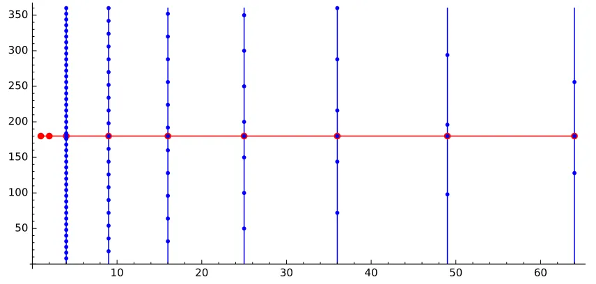
The functionsψ1,ψ2are themselves based on an intermediate construction of a functionΨ:[N]×
[K]→R, forK=Θ(N2/3), depicted pictorially inFigure 1below. The functionΨ, defined in the proof ofLemma 4.2, combines the constructions ofω fromLemma 3.1andηkfromLemma 4.1.
Figure 1: A visualization of the support of the functionΨ(m,k), forN=360 andK=64. The horizontal axis represents values ofk=1, . . .Kand the vertical axis represents values ofm=1, . . . ,N. Red dots indicate values in the support of the functionω(k)1m=N/2, while blue dots indicate values in the support
of the functionω(k)ηk(m)1k≥3. When red dots and blue dots overlap, they “cancel out,” in the sense that
a point with both a red and a blue dot isnotin the support ofΨ.
Together, the functionsψ1,ψ2yield the desired dual polynomial for ColN,R.
Theorem 4.3. Let N>0be an integer multiple of 4. For R≥N, there exists an explicit(1−6δ,d)-dual polynomialψ forColN,Rfor d=Ω(δ1/3N1/3).
constructing an explicit approximating polynomial for ColN,Rof the appropriate degree, by building on
the ideas underlying the quantum query algorithm of Brassard et al. [17].
Proof ofTheorem 4.3, assumingLemma 4.2. Let
a=
∑
x∈T1 ψ1(x)
and let
b=
∑
x∈T2
|ψ2(x)|=−
∑
x∈T2ψ2(x),
whereψ1andψ2are as inLemma 4.2. Letψ(x) =aψ1(x) +bψ2(x). By Property 5 ofLemma 4.2and Lemma 4.5below,ψ also has pure high degree at leastd. So we need only show thatψ has correlation at
least 1−6δ with ColN,R. To this end, note the following.
1.
∑
x∈T1
ψ(x) =a2>(1−δ) 2
4 . This inequality uses Properties 1 and 4 ofLemma 4.2.
2. −
∑
x∈T2
ψ(x) =b2>(1−δ) 2
4 . This inequality uses Properties 2 and 4 ofLemma 4.2.
3.
∑
x∈B
|ψ(x)| ≤a
∑
x∈B\RN/2,2,1|ψ1(x)|+b
∑
x∈B\RN/2,2,1|ψ2(x)| ≤(a+b)δ.
Here, the first inequality exploits the fact that
∑
x∈RN/2,2,1
|ψ(x)|=
∑
x∈RN/2,2,1|a·ψ1(x) +b·ψ2(x)|=0. (4.1)
The last equality in (4.1) holds because, for allx∈RN/2,2,1,
a·ψ1(x) +b·ψ2(x) =
∑
x0∈T1 ψ1(x0)
!
·ψ1(x) + −
∑
x0∈T2 ψ2(x0)
!
ψ2(x)
=
∑
x0∈R
N/2,2,1 ψ2(x0)
·ψ1(x) +
−
∑
x0∈R
N/2,2,1 ψ1(x0)
ψ2(x)
=
∑
x0∈R
N/2,2,1 ψ2(x0)
1
|RN/2,2,1|x0∈R
∑
N/2,2,1 ψ1(x0)
+
−
∑
x0∈R
N/2,2,1 ψ1(x0)
1
|RN/2,2,1|x0∈R
∑
N/2,2,1 ψ2(x0)
=0,
Thus, the correlation ofψwith ColN,Ris
∑
x∈T1
ψ(x)−
∑
x∈T2
ψ(x)−
∑
x∈B
|ψ(x)| ≥a2+b2−(a+b)δ
≥1
2−2δ ≥(1−6δ)· kψk1,
where the final inequality holds becausekψk1≤a2+b2+ (a+b)δ≤1/2+δ.
Lemma 4.5. Letψ1,ψ2:{−1,1}n→ {−1,1}each have pure high degree at least d. Then
ψ=ψ1+ψ2 also has pure high degree at least d.
Proof. LetS⊆[n]with|S| ≤d. Then
∑
x∈{−1,1}n
ψ(x)χS(x) =
∑
x∈{−1,1}nψ1(x)χS(x) +
∑
x∈{−1,1}nψ2(x)χS(x) =0.
What now remains is to proveLemma 4.2, i. e., to construct the intermediate functionsψ1,ψ2that were used to proveTheorem 4.3.
Proof ofLemma 4.2. Letζ be the constant fromLemma 3.1, letρ be the constant fromLemma 4.1, and letδ0=1/2. Set
K=2
ρN
ζ
2/3
δ0 δ
1/3
and let d=1
2ρ
1/3
ζ2/3(δ0)1/6δ1/3N1/3=Ω(δ1/3N1/3),
noting thatd≤ζ(δ/8)1/2K1/2 andd≤ρ(δ0)1/2N/k for every k≤K. Letω:{1, . . . ,K} →R, with
correlation constantδ/8, andη3, . . . ,ηK:{1, . . . ,N} →R, with correlation constant δ0, be as in the
conclusions of those lemmas.
We start by defining a functionΨ:[N]×[K]→Ras follows.
Ψ(m,k) =ω(k)·1m=N/2− ω(k)
ηk(N/2)1k≥3·ηk(m).
Here,
1m=N/2=
(
1 ifm=N/2,
0 otherwise, and 1k≥3= (
1 ifk≥3,
0 otherwise.
To help the reader build intuition about the functionΨ, we present inFigure 1 a visualization of its support.
We first show how to useΨto construct the polynomialψ1. Analogously to our construction ofφ,
we wantψ1to place a total weight ofΨ(m,a)on each setRm,a,1. Recall from our overview inSection 2.5
that we think of
ψ1=ψ0+
∑
invalid triples(N/2,a,1)ψN00/2,a,1,
whereψ0looks like the simpler “first stage” dual polynomialφfrom our informal overview (which we
divideN. This structure underlies our construction ofΨ, where we add multiples of the polynomials ηk(m)to cancel out the weightω(k)places on invalid triples.
Now we construct and analyze the polynomialψ1. Define
ˆ
ψ1(x) =
Ψ(m,k)/|Rm,k,1| ifx∈Rm,k,1\T1, Ψ(N/2,1)/|T1| ifx∈T1,
0 otherwise.
Notice that ˆψ1is well-defined, because anyx6∈T1is inRm,k,1for at most one triple(m,k,1). We collect
several calculations with ˆψ1. First,
∑
x∈T1
ˆ
ψ1(x) =Ψ(N/2,1) =ω(1)> 1
−δ/8
2 ,
−
∑
x∈RN/2,2,1
ˆ
ψ1(x) =−Ψ(N/2,2) =−ω(2)>1−δ/8
2 ,
and
∑
x∈B\RN/2,2,1
|ψˆ1(x)|=
∑
{(m,k):k|m}\{(N/2,1),(N/2,2)}
|Ψ(m,k)|
=
K
∑
k=3
ω(k) ηk(N/2)
bN/2kc
∑
i=1
|ηk(2ki)|
≤4
K
∑
k=3
|ω(k)|
≤ δ 2,
where the penultimate inequality exploits Properties 2 and 3 ofLemma 4.1, and the final inequality exploits Properties 1-3 ofLemma 3.1.
Noting that|ω(1)|+|ω(2)| ≤1, it follows thatkψ1ˆ k1≤1+δ/2. So settingψ1=ψ1/ˆ kψ1ˆ k1, it is
immediate thatψ1satisfies the first three properties in the statement of the lemma.ψ1also satisfies the
fourth property, since for anyx∈T2,ψ1(x) =Ψ(N,2)/|T2|=0.
Now we will show that ˆψ1, and henceψ1, has pure high degree at leastd. We require two observations.
a) Ψis supported on(m,k)for whichk|m. To see this, note first that for anyk≥3,
Ψ(N/2,k) =ω(k)− ω(k)
ηk(N/2)·ηk(N/2) =0.
The claim now follows from Property 1 ofLemma 4.1, combined with the fact that 2|N.
b) Ψ(m,1)is nonzero only form=N/2, and hence
∑
x∈T1
ˆ
ψ1(x) =Ψ(N/2,1) = N
∑
m=1
Fix anyS⊆[n]with|S| ≤d. LetQ(m,k)be a polynomial of degree at mostdin each variable such that, for all pairs(m,k)withk|m,
Q(m,k) =Ex∈Rm,k,1[χS(x)].
The existence of such a bivariate polynomialQis guaranteed byLemma 2.5. Then the previous two observations together imply that
∑
x∈{−1,1}n
ˆ
ψ1(x)χS(x) = N
∑
m=1 N
∑
k=1
Ψ(m,k)Q(m,k). (4.2)
We remark that a key point is the derivation of (4.2) is that we have no control over the evaluations
Q(m,k)whenkdoes not dividem, yet this is rendered irrelevant becauseΨ(m,k) =0 for all such pairs. The right hand side of (4.2) equals
K
∑
k=1
ω(k)Q(N/2,k)− K
∑
k=3 ω(k)
ηk(N/2) ηk(N/2)Q(N/2,k) +
bN/2kc
∑
i=1
ηk(2ik)Q(2ik,k)
!
. (4.3)
The first sum in (4.3) is zero byLemma 3.1sinceQ(N/2,k)is a polynomial of degree at mostdink. The second sum is also zero because for each fixedk,Q(r,k)is a polynomial of degree at mostdin the variabler, and hence the term in parentheses is zero byLemma 4.1(Parts 1 and 4). Thus ˆψ1has pure
high degree at leastd.
The construction ofψ2is similar. This time, we let
ˆ
ψ2(x) =
Ψ(m,k)/|Rm,k,2| ifx∈Rm,k,2\T2, Ψ(N/2,2)/|T2| ifx∈T2,
0 otherwise.
Note that ˆψ2is well-defined, because anyx6∈T2is inRm,k,2for at most one triple(m,k,2). We define ψ2=ψ2/ˆ kψ2ˆ k1. Showing thatψ2satisfies Properties 1-4 of the lemma follows from the same calculations
we used forψ1.
To show thatψ2has pure high degree at leastd, we require the following additional observations.
c) Ψis supported on pairs(m,k)for whichk|mand 2|(N−m). To see the latter property, note that if Ψ(m,k)6=0, thenmis even (this holds becauseN/2 is even, which follows from our requirement that Nis a multiple of 4), and henceN−mis as well.
d) Ψ(m,2)is nonzero only form=N/2. It follows that∑x∈T2ψˆ2(x) =Ψ(N/2,2) =∑ N
m=1Ψ(m,2).
With these observations in hand, showing thatψ2has pure high degreedthen follows from calculations
analogous to the ones we used forψ1.
Finally, the fact that ψ1 and ψ2 satisfy Properties 6, 7, and 8 of the lemma follows from their
definitions, combined with the fact thatRN/2,1,2=RN/2,2,1. In fact,∑x∈T1ψ1(x)equalsΨ(N/2,1), while
∑
also equalsΨ(N/2,1), giving Property 6. Similarly,∑x∈T2ψ2(x)equalsΨ(N/2,2), while
∑
x∈RN/2,1,2 ψ1(x)
also equalsΨ(N/2,1). This completes the proof.
5
A dual polynomial for E
LEMENTD
ISTINCTNESSIn this section, we give a generic construction showing how to transform any dual polynomial for COLLISIONinto a dual polynomial for ELEMENTDISTINCTNESS.
We first recall the reduction from COLLISION to ELEMENT DISTINCTNESS given in [5].4 The reduction shows how to turn a polynomialpapproximating EDM,Rinto a polynomialqapproximating
ColN,R, withN≈M2and degq≤degp.
We illustrate the reduction forN=M2/12. Let p:{−1,1}m→ {−1,1}be an(1/6)-approximation
of EDM,R, withm=MlogR. Define a polynomialq:{−1,1}n→ {−1,1}forn=NlogRby
q(y1, . . . ,yN) = 1N
M
∑
1≤i1<i2<···<iM≤N
p(yi1,yi2, . . . ,yiM).
That is,q(y)is the expected value of p(x)wherexis the concatenation of a random subset ofMof the blocksy1, . . . ,yN. To simplify notation, for a setS={i1,i2, . . . ,iM}, lety|S= (yi1,yi2, . . . ,yiM). Note that
degq≤degp. Moreover, sinceqis an average of values in[−7/6,7/6], it is always in[−7/6,7/6]itself. To finish arguing thatqis a(1/3)-approximation to ColN,R, we consider two cases.
1. Ify∈T1, i. e.,yis a 1-to-1 input, theny|S is always 1-to-1. Hencep(y|S)∈[5/6,7/6]for every
subset of indices, soq(y)∈[2/3,4/3].
2. Ify∈T2, i. e.,yis a 2-to-1 input, then with high probabilityy|Sis not 1-to-1. This follows from the
“birthday bound”:
Pr
|S|=M[ED(y
|S) =1]≤exp(−M2/4N)≤
1 12.
Therefore,q(y)≤(11/12)(−5/6) + (1/12)(7/6)≤ −2/3.
The construction we give in this section takes a dual view of the reduction above. Namely, we show how to transform a dual polynomialψ for ColN,R into a dual polynomialϕ for EDM,R, withM2≈N. In
the primal reduction, we constructedq(y)from p(x)by averagingpover all subsets of sizeM. The right analogue in the dual reduction is to constructϕ(x)by averagingψ(y)over a carefully constructed set of extensionsfromxto a longer inputy. In particular,ϕ(x)averagesψ(y)over allyfor whichxcould have
been produced by taking a subset ofMblocks ofy. We give this reduction formally below.
4While the reduction given in Aaronson and Shi’s paper is stated in terms of quantum query algorithms, it is straightforward
Theorem 5.1. Let ψ :{−1,1}n→ {−1,1} be a(1−δ,d)-dual polynomial forColN,R. Thenψ can be used to constructϕ:{−1,1}m→ {−1,1}that is an(1−2δ,d)-dual polynomial forEDM,R when M≥2pNlog(2/δ).
Corollary 5.2. For anyδ >0, there is an explicit(1−δ,d)-dual polynomial forEDM,Rwith
d=Ω
δ
log(1/δ)
1/3
M2/3
!
.
Remark 5.3. The dependence ofCorollary 5.2onδ is essentially tight forδ =O(M−2). SeeSection 7
for details.
Proof ofTheorem 5.1. Given a set S={i1, . . . ,iM} ⊂[N]withi1<i2<· · ·<iM and a bit stringy=
(y1, . . . ,yN)∈ {−1,1}n, define the restriction ofyto the setS, denoted byy|S∈ {−1,1}m, to be the string
of lengthm=MlogRobtained by concatenating the blocksyifori∈S, i. e.,y|S= (yi1,yi2, . . . ,yiM). Given
a bit stringx∈ {−1,1}m, define the multiset of extensions ofx, denoted by ext(x), to be the N M
RN−M
stringsy∈ {−1,1}n wherey|
S=x for some|S|=M. Restrictions and extensions are related by the
equality of the multisets
{(x,y):x∈ {−1,1}m,
y∈ext(x)}={(x,y):y∈ {−1,1}n,x=
y|Sfor some|S|=m}. (5.1)
Forx∈ {−1,1}m, define the polynomial
ϕ(x) = 1N M
∑
y∈ext(x)
ψ(y).
Letϕ(x) =0 forx∈ {−/ 1,1}m. We claim thatϕis a good dual polynomial for the ELEMENT DISTINCT -NESSfunction ED, which requires us to show
1. ∑x∈{−1,1}mϕ(x)ED(x)>(1−2δ)·∑x∈{−1,1}m|ϕ(x)|, and
2. ∑x∈{−1,1}mϕ(x)χS(x) =0 for all|S| ≤d.
To verify the first property, define
A(y) = 1N
M
∑
|S|=M
ED(y|S).
We collect a few observations aboutA.
1. |A(y)| ≤1 for ally.
2. Ify∈T1, thenA(y) =1.
3. Ify∈T2, then
Pr
|S|=M[ED(y|S) =1]≤exp(−M 2/4N).
Hence,
Therefore we get
∑
x∈{−1,1}m
ϕ(x)ED(x) = 1N M
∑
x∈{−1,1}my∈
∑
ext(x)ψ(y)ED(x)
= 1N
M
∑
y∈{−1,1}n|S
∑
|=Mψ(y)ED(y|S) by (5.1)
=
∑
y∈{−1,1}n
A(y)ψ(y) by definition ofA.
By observations (1)-(3) aboutA, this expression is
≥
∑
y∈T1
ψ(y)−
∑
y∈T2ψ(y)−
∑
y∈B|ψ(y)|
!
−δ
∑
y∈T2|ψ(y)|
≥(1−2δ)
∑
y∈{−1,1}n|ψ(y)| asψ is a dual polynomial for ColN,R
= (1−2δ)
∑
y∈{−1,1}n1
N M
∑
|S|=M
|ψ(y)|
≥1−2δ
N M
∑
x∈{−1,1}my∈
∑
ext(x)|ψ(y)| by (5.1)
≥(1−2δ)
∑
x∈{−1,1}m|ϕ(x)|.
For the second property, letT be a subset of[N]with|T| ≤d. Then
∑
x∈{−1,1}m
ϕ(x)χT(x) = 1N M
∑
x∈{−1,1}my∈
∑
ext(x)ψ(y)χT(x)
= 1N
M
∑
|S|=M
∑
y∈{−1,1}n
ψ(y)χT(y|S) by (5.1)
= 1N
M
∑
|S|=M
∑
y∈{−1,1}n
ψ(y)χT|S(y)
=0,
whereT|Sdenotes the subset ofT contained in the blocks specified byS.
6
On complementary slackness
Recalling that any bounded-error quantum query algorithm can be converted into an approximating polynomial [11], the collision-finding algorithm of Brassard, Høyer, and Tapp [17] yields an explicit, asymptotically optimal approximating polynomial for ColN,R. We describe this polynomialpbelow.
Recall that any approximating polynomial for ColN,R represents a feasible solution to the primal
for ColN,R, then complementary slackness would imply that the optimal dual polynomialψ for ColN,Ris
supported on the points corresponding to constraints made tight byp. That is,ψ :{−1,1}n→ {−1,1}is
supported onx∈ {−1,1}nfor which|p(x)−Col(x)|=
ε. We refer to these as themaximum-error points
ofp.
While we do not know whether pis an exactly optimal approximating polynomial for ColN,R, we
might still expect that an approximate version of complementary slackness holds, in the sense that a “good” dual polynomial should place all or most of its weight on points that are “nearly” maximum-error points ofp. Indeed, this intuition has proven accurate for all of the dual polynomials constructed in prior work, including for symmetric functions (see [19, Section 4.5]), block-composed functions (see [48, Section 1.2.4]), and the intersection of two majorities [41]. Below, we argue thatk-to-1 inputs are nearly maximum-error points forp, which explains why our dual polynomials for collision are supported on inputs that are roughlyk-to-1, in addition to why these inputs play a prominent role in the original symmetrization-based proof.
An asymptotically optimal approximationpforColN,R. For a subsetS⊂[N], define
crossS:{−1,1}n→Rvia
crossS(x1, . . . ,xN) =|{i∈S,j∈/S:xi=xj}|=
∑
i∈S,j6∈SEQ(xi,xj),
where EQ denotes the equality function. That is,crossS(x)counts the number of cross-collisions between
indices inSand indices outside ofS. Notice that EQ(xi,xj)is a function of only 2·logRvariables, and
hencecrossS(x1, . . . ,xN)is exactly computed by a polynomial of degree 2·logR.
In addition, for a subsetS⊂[N], define the functionIED,S(x1, . . . ,xN)to be 1 ifxi6=xjfor all pairs i,j∈Swithi6= j, and 0 otherwise. That is,IED,Sindicates whetherxis 1-to-1 on the indices inS. Notice
thatIED,Sis a function of only|S| ·logRvariables, and hence is exactly computed by a polynomial of
degree|S| ·logR.
For the remainder of the discussion, letr=N1/3—we focus on the quantitycrossS(x)when|S|=r.
We will need the following simple observations.
1. Ifx∈T1, i. e.,xis a 1-to-1 input, thencrossS(x) =0 andIED,S(x) =1 for anyS.
2. Ifx∈T2, i. e.,xis a 2-to-1 input, thenIED,S(x) =1=⇒crossS(x) =r.
3. Ifx∈T2, then, over the random choice ofS,IED,S(x) =0 with probability at most(N/2)·(r/N)2≤ N−1/3.
4. For allx∈ {−1,1}n,
IED,S(x) =1=⇒crossS(x)≤N−r.
LetTd:R→Rdenote the degree-dChebyshev polynomial of the first kind. This polynomial has the following properties.
a) Td(x)∈[−1,1]forx∈[−1,1].
c) The extreme points ofTd in[−1,1]are the degree-d Chebyshev nodes, which take the form cos(iπ/d)
for 0≤i≤d.
Truncating the Taylor expansion of cos(x) =1−x2/2+. . . after the quadratic term, one sees that the Chebyshev nodes are well-approximated via the expression cos(iπ/d)≈1−(ci2/d2)for some constant
c.
Applying an appropriate affine transformation toTd, we obtain a polynomialAd with the following properties.
a) Ad(0) =1.
b) Ad(i)∈[−1,−3/4]for all real numbersi∈[1,d2/M].
c) Ad(i)∈[−1,1]for all real numbersi∈[0,d2/M].
d) The extreme points ofAd are well approximated by the pointsc·i2fori∈ {0,1, . . . ,bd·M−1/2c}.
LetpS(x) =IED,S(x)·Ad(crossS(x1, . . . ,xN)/r)ford=100·M·N1/3, and let
p(x) =E|S|=r[pS(x)] =
1
N r
∑
|S|=r pS(x).
Thenpis a polynomial of degree|S|logR+2·d·logR=O(N1/3logR). We argue that papproximates ColN,Rto errorε for someε ≤1/3. The analysis falls into three cases.
Case 1: Forx∈T1,pS(x) =Ad(0) =−1 for allS, where the first equality follows from Property 1 above.
So p(x) =E|S|=r[pS(x)] =1.
Case 2: For x∈T2, IED,S(x) =1=⇒ pS(x) =Ad(1)∈[−1,−3/4], where the equality follows from
Property 2 above. Meanwhile, IED,S(x)=6 1=⇒ pS(x) =0. Combining these two facts with
Property 3 above establishes that p(x) =E|S|=r[pS(x)]∈[−1,−2/3].
Case 3: Forx∈ {−1,1}n,pS(x)∈[−1,1]. This follows from Property 4 above.
Identifying maximum-error points ofp. For any fixedS, the maximum-error points ofpSare well-approximated by thex∈ {1,1}nfor which the following two equations hold:
crossS(x) =c·i2·rfor somei∈ {0,1, . . . ,bd·M−1/2c} (6.1)
and
IED,S(x) =1. (6.2)
(This follows from the fact that the extreme points ofAdare roughly of the formc·i2for 0≤i≤d·M−1/2).
Consider anykof the formk=c·i2+1 for somei∈ {0,1, . . . ,bd·M−1/2c}, such thatk=o(N1/3). Consider anyx∈Tk; we claim thatxsatisfies (6.1) and (6.2) with probability 1−o(1)over choice ofS. To see this, observe that the probability thatIED,S(xS) =0 is at most(N/k)·k2·(r/N)2=k·r2/N=o(1).
And ifIED,S(xS)6=0, then the number of cross-collisions is exactly
crossS(x1, . . . ,xN) =r·(k−1).
Whenktakes the formk=c·i2+1, this means thatxsatisfies (6.1). Hence,xhas nearly maximal error even for the averaged polynomialp.
7
On the tightness of
Theorem 4.3
and
Corollary 5.2
To complementTheorem 4.3, we construct an approximating polynomial that gives a nearly matching upper bound on the approximate degree of ColN,R. The construction is a refinement of the approximating
polynomial given inSection 6.
Proposition 7.1. For0≤δ≤1/N, there exists a polynomial p of degree O(δ1/3N1/3logR)that(1−δ) -approximatesColN,R.
Proof sketch. SeeSection 6for the construction of an approximating polynomial of degreeO(N1/3logR)
in the case whereδ is constant. In order to obtain an improved upper bound for vanishingδ, we make the
following changes to that construction.
1. We instead chooser=δ1/3N1/3. Now ifxis a 2-1 input, the probability over the random choice
of the set S of obtaining a collision inside S, i. e., the probability that IED,S =0, is at most
(N/2)·(r/N)2≤δ/2.
2. We instead letAd be an affine transformation of a Chebyshev polynomial with the following
properties for some constantM:
• Ad(0)≥δ/2,
• Ad(i)∈[−1,−δ/2]fori∈[1,d2/Mδ],
• Ad(i)∈[−1,1]forx∈[0,d2/Mδ].
3. Settingd=100·M·rensures that the polynomialphas degreeO(δ1/3N1/3logR)and is a(1−δ)
-approximation of ColN,R.
We now show thatCorollary 5.2is tight up to a factor of logR, whenδ ≤1/M2. This gives mild
evidence that the lower bound has the right dependence on both parametersM,δ for vanishingδ.