www.theoryofcomputing.org
Linear-Time Algorithm for Quantum 2SAT
Itai Arad
∗Miklos Santha
∗†Aarthi Sundaram
∗‡Shengyu Zhang
∗§Received May 16, 2016; Revised August 22, 2017; Published March 9, 2018
Abstract: A well-known result about satisfiability theory is that the 2-SAT problem can be solved in linear time, despite theNP-hardness of the 3-SAT problem. In the quantum 2-SAT problem, we are given a family of 2-qubit projectorsΠi j on a system ofnqubits, and the
task is to decide whether the HamiltonianH=∑ Πi j has a 0-eigenvalue, or all eigenvalues
are greater than 1/nαfor some
α=O(1). The problem is not only a natural extension of
the classical 2-SAT problem to the quantum case, but is also equivalent to the problem of finding a ground state of 2-local frustration-free Hamiltonians of spin 1/2, a well-studied model believed to capture certain key properties in modern condensed matter physics. Bravyi has shown that the quantum 2-SAT problem has a deterministic algorithm of complexity
O(n4)in the algebraic model of computation where every arithmetic operation on complex numbers can be performed in unit time, andnis the number of variables. In this paper we give a deterministic algorithm in the algebraic model with running timeO(n+m), wherem
is the number of local projectors, therefore achieving the best possible complexity in that model. We also show that if in the input every number has a constant size representation then the bit complexity of our algorithm isO((n+m)M(n)), whereM(n)denotes the complexity of multiplying twon-bit integers.
ACM Classification:F.2
AMS Classification:68Q25, 81P68
Key words and phrases:quantum satisfiability, davis-putnam procedure, linear time algorithm
Aconference versionof this paper appeared in the Proceedings of the 43rd International Colloquium on Automata, Languages and Programming (ICALP’16), 2016 [1].
∗Supported by the Singapore Ministry of Education and the National Research Foundation, also under the Tier 3 Grant
MOE2012-T3-1-009; by the European Commission IST STREP project Quantum Algorithms (QALGO) 600700; and the French ANR Blanc Program Contract ANR-12-BS02-005.
†Also thanks STIAS for their hospitality during October and November 2015.
1
Introduction
Various formulations of the satisfiability problem of Boolean formulae arguably constitute the centerpiece of classical complexity theory. In particular, a great amount of attention has been paid to the SAT problem, in which we are given a formula in the form of a conjunction ofclauses, where each clause is a disjunction ofliterals(variables or negated variables), and the task is to find a satisfying assignment if there is one, or determine that none exists when the formula is unsatisfiable. In the case of thek-SAT problem, wherek
is a positive integer, the number of literals in each clause is at mostk. Whilek-SAT is anNP-complete problem [7,16,21] whenk≥3, the 2-SAT problem is well-known to be efficiently solvable.
Polynomial time algorithms for 2-SAT come in various flavours. Let us suppose that the input formula hasnvariables andmclauses. The algorithm of Krom [19] based on the resolution principle and on transitive closure computation decides if the formula is satisfiable in timeO(n3) and finds a satisfying assignment in timeO(n4). The limited backtracking technique of Even, Itai and Shamir [11]
has linear time complexity inm, as well as the elegant procedure of Aspvall, Plass and Tarjan [2] based on computing strongly connected components in a graph. A particularly simple randomized procedure of complexityO(n2)is described by Papadimitriou [22].
For our purposes the Davis-Putnam procedure [9] is of singular importance. This is a resolution-principle based general SAT solving algorithm, which with its refinement due to Davis, Putnam, Logemann and Loveland [8], forms the basis for the most efficient SAT solvers even today. While on general SAT instances it works in exponential time, on 2-SAT formulae it is of polynomial complexity.
The high level description of the procedure for 2-SAT is relatively simple. Let us suppose that our formulaφ only contains clauses with two literals. Pick an arbitrary unassigned variablexiand assign
xi=0. The formula is simplified: a clause(xi¯ ∨xj)becomes true and therefore can be removed, and a
clause(xi∨xj)forcesxj=1. This can be, in turn, propagated to other clauses to further simplify the
formula until a contradiction is found or no more propagation is possible. If no contradiction is found and the propagation stops with the simplified formulaφ0, then we recurse on the satisfiability ofφ0.
Otherwise, when a contradiction is found, that is, at some point the propagation assigns two different values to the same variable, we reverse the choice made forxi, and propagate the new choicexi=1. If this also leads to a contradiction we declareφ to be unsatisfiable, otherwise we recurse on the result of
this propagation, the simplified formulaφ1.
There is a deep and profound link betweenk-SAT formulas andk-local Hamiltonians, the central objects of condensed matter physics. Ak-local Hamiltonian onnqubits is a Hermitian operator of the formH=∑mi=1hi, where eachhiis individually a Hermitian operator acting non-trivially on at mostk
qubits. Local Hamiltonians model the local interactions between quantum spins. Of central importance are the eigenstates of the Hamiltonian that correspond to its minimal eigenvalue. These are calledground states, and their associated eigenvalue is known as theground energy. Ground states govern much of the low temperature physics of the system, such as quantum phase transitions and collective quantum phenomena [24,25]. Finding a ground state of a local Hamiltonian shares important similarities with the
attention has been devoted to understanding this structure, revealing a rich and intricate behaviour such as area laws [10] and topological order [17].
The connection between classicalk-SAT and quantum local Hamiltonians was formalized by Ki-taev [18] who introduced thek-local Hamiltonian problem. We are given ak-local HamiltonianH, along with two constantsa<bsuch that b−a>1/nα for some constant
α, and a promise that the ground
energy is at mosta(the YES case) or is at leastb (the NO case). Our task is to decide which case holds. Given a quantum state|ψi, the energy of a local termhψ|hi|ψican be viewed as a measure of
how much|ψi“violates”hi, hence the ground energy is the quantum analog of the minimal number of
violations in a classicalk-SAT formula. Therefore, in spirit, thek-local Hamiltonian problem corresponds to MAX-k-SAT, and indeed Kitaev has shown [18] that 5-local Hamiltonian isQMA-complete, where the complexity classQMAis the quantum analogue of classical classMA, the probabilistic version ofNP.
The problem quantum k-SAT, the quantum analogue of k-SAT, is a close relative of thek-local Hamiltonian problem. Here we are given a k-local Hamiltonian that is made of k-local projectors,
H=∑mi=1Qi, and we are asked whether the ground energy is 0 or it is greater thanb=1/nα for some
constantα. Notice that in the YES case, the energy of each projector at a ground state is necessarily 0 because, by definition, projectors are non-negative operators. Classically, this corresponds to a perfectly satisfiable formula. Physically, this is an example of afrustration-freeHamiltonian, in which a global ground state is also a ground state of every local term. Bravyi [4] has shown that quantumk-SAT is
QMA1-complete fork≥4, whereQMA1stands forQMAwith one-sided error (that is on YES instances the verifier accepts with probability 1). TheQMA1-completeness of quantum 3-SAT was recently proven by Gosset and Nagaj [12].
This paper is concerned with the quantum 2-SAT problem, which we will also denote simply by Q2SAT. One major result concerning this problem is due to Bravyi [4], who has proven that it belongs to the complexity classP. More precisely, he has proven that Q2SAT can be decided by a deterministic algorithm in timeO(n4) in thealgebraic model of computation, where every arithmetic operation on complex numbers can be performed in unit time. In addition, on satisfiable instances he could construct a ground state that has a polynomial classical description. In the case of Q2SAT, the Hamiltonian is given as a sum of 2-qubits projectors; each projector is defined on a 4-dimensional Hilbert space and can therefore be of rank 1, 2 or 3. In this paper, we give an algorithm for Q2SAT oflinearcomplexity.
Theorem 1.1. In the algebraic model of computation there is a deterministic algorithm forQ2SATwhose running time is O(n+m), where n is the number of variables and m is the number of local terms in the Hamiltonian.
Our algorithm shares the same trial and error approach of the Davis-Putnam procedure for classical 2-SAT, but handles many of the difficulties arising in the quantum setting. Firstly, a ground state of the input to Q2SAT may be entangled, a feature that classical 2-SAT does not have. Thus the idea of setting some qubit to a certain state and propagating from there does not have foundation in the first place. Indeed, if a rank-3 projection leaves the only allowed state entangled, then any ground state is entangled in those two qubits. We account for this by showing aproduct-state theorem, which asserts that for any frustration-free Q2SAT instanceHthat contains only rank-1 and rank-2 projectors, there always exists a ground state in the form of a tensor product ofsingle-qubitstates.
This structural theorem grants us the following approach: We try some candidate solution|ψiion a
explored part and recurse on the rest of the graph. If a contradiction is found, then we can identify two candidates(i,|ψii)and(j,|φij)such that either assigning|ψii to qubitior assigning|φij to qubit jis
correct, if there exists a solution at all. More details follow next.
To illustrate the main idea of our algorithm, let us assume, for simplicity, that the system is only made of rank-1 projectors. Consider, then a rank-1 projector in the system, say,Π12=|ψihψ|over
qubits 1 and 2. The product-state theorem implies that it suffices to search for a product ground state. Thus on the first two qubits, we are looking for states|αi,|βisuch that(hα| ⊗ hβ|)Π12(|αi ⊗ |βi) =0,
which is equivalent tohα| ⊗ hβ| · |ψi=0. In other words, we look for a product state|αi ⊗ |βithat is
perpendicular to|ψi. Assume that we have assigned qubit 1 with the state|αiand we are looking for a state|βifor qubit 2. The important point, which enables us to solve Q2SAT efficiently, is that just like in
the classical case, there are only two possibilities: (i) for any|βi, the state|αi ⊗ |βiis perpendicular to
|ψi, or (ii) there is only one state|βi(up to an overall complex phase), for which(hα| ⊗ hβ|)· |ψi=0. The first case happens if and only if|ψiis by itself a product state of the form|ψi=|α⊥i ⊗ |ξi, where
|α⊥iis perpendicular to|αiand|ξiis arbitrary. If the second case happens, we say that the state|αiis
propagated to the state|βiby the constraint state|ψi.
The above dichotomy enables us to propagate a product state|si on part of the system until we either reach a contradiction, or find that no further propagation is possible and we are left with a smaller HamiltonianH0. This smaller Hamiltonian consists of a subset of the original projectorswithout introducing new projectors. This crucial fact implies that, analogous to the classical case, the original HamiltonianHis satisfiable if and only if the smaller HamiltonianH0is satisfiable.
We still need to specify how the state|αiis chosen to initialize the propagation. An idea is to begin
with projectors|ψihψ|for which|ψiis a product state|γi ⊗ |δi. In such cases a product state solution
must either have|γ⊥iat the first qubit or|δ⊥iat the second. To maintain a linear running time, we
propagate these two choices simultaneously until one of the propagations stops without contradiction, in which case the corresponding qubit assignment is made final. If both propagations end with contradictions, the input is rejected.
The more interesting case of the algorithm happens when we have only entangled rank-1 projectors. What should our initial state be then? We make an arbitrary assignment (say,|0i) to any of the still unassigned qubits and propagate this choice. If the propagation ends without contradiction, we recurse. If a contradiction is found then we confront a challenging problem. In the classical case we could reverse our choice, sayx0=0, and try the other possibility,x0=1. But in the quantum case we have an infinite
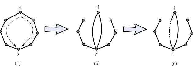
number of potential assignment choices. The solution is found by the following observation: Whenever a contradiction is reached, it can be attributed to a cycle of entangled projectors in which the assignment has propagated from qubitialong the cycle and returned to it with another value (seeFigure 1(a)). Then using the technique of “sliding,” which was introduced in Ref. [15], one can show that this cycle is equivalent to a system of one double edge and a “tail” (seeFigure 1(b)). Using a simple structure lemma, we are guaranteed that at least one of the projectors of the double edge can be turned into a product state projector, which, as in the previous stage, gives us only two possible free choices.
Figure 1: Handling a contradicting cycle: (a) we slide edges that touchialong the two paths to juntil (b) we get a double edge with two “tails.” (c) we use a structure lemma to deduce that at least one of these edges can be written as a product projector (a dashed edge).
made. Bravyi [4] suggests considering bounded degree algebraic numbers, in which case the length of the representations and the cost of the operations can be analyzed by considering their bit-wise costs, termed thebit complexity. For the sake of completeness, following the thread of working within the framework of bounded algebraic numbers, we provide an analysis of the bit complexity of our algorithm in the final section of the paper. More precisely, we prove that if in the input every number has a constant size representation then the bit complexity of our algorithm isO((n+m)M(n)), whereM(n)denotes the complexity of multiplying twon-bit integers. Finding an algorithm with a better bit complexity seems to be a hard problem and we leave this challenge as an open problem.
Classically, Davis-Putnam [9] and DPLL algorithms [8] are widely-used heuristics, forming the basis of today’s most efficient solvers for general SAT. For quantumk-SAT, it could also be a good heuristic if we try to find product-state solutions, and in that respect our algorithm makes the first-step exploration. Simultaneously albeit independently from our work de Beaudrap and Gharibian [3] also presented a linear time algorithm for quantum 2SAT. The main difference between the two algorithms is how they deal with instances having only entangled rank-1 projectors. Contrarily to us, [3] handles these instances by using transfer matrix techniques to find discretizing cycles [20].
2
Preliminaries
2.1 Notation
We will use the notation[n] ={1, . . . ,n}. For a graphG= (V,E), and for a subsetU⊆V of the vertices, we denote byG(U)the subgraph induced byU. Our Hilbert space is defined overnqubits, and is written
asH=H1⊗H2⊗ · · · ⊗Hn, whereHiis the two-dimensional Hilbert space of theithqubit. We shall
often write|αii to emphasize that the 1-qubit state|αilives inHi. Similarly,|ψii j denotes a 2-qubit
state that lives inHi⊗Hj. For a 1-qubit state|αi=α0|0i+α1|1i, we define itsperpendicular stateas
|α⊥i=α¯1|0i −α¯0|1i, where ¯α denotes the complex conjugate ofα.
A 2-local projectoron qubitsi6=jis a projector of the formΠi j=Πˆi j⊗Irest, where ˆΠi j is a 2-qubit
projector working onHi⊗Hj andIrest is the identity operator on the rest of the system. Similarly, a
working onHiandIrestis the identity operator on the rest of the system. We define therankof a 2-local
projectorΠi j=Πˆi j⊗Irestto be the dimension of the subspace that ˆΠi jprojects to, and we denote it by rank(Πi j). The rank of a 1-local projector is defined analogously. The 2-local projectors of rank 3 and
the 1-local projectors of rank 1 are considered to be ofmaximalrank. A 2-local projectorΠi j=Πˆi j⊗Irest
of rank 1 where ˆΠi j=|ψihψ|i j is calledentangledif|ψiis an entangled state, and it is called aproduct
projector if|ψiis a product state.Recall that a 2-qubit state|ψii jis a product state if it can be written as a
tensor product of 2 single-qubit states|ψii j=|ψ1ii⊗ |ψ2ij; and a 2-qubit state which is not a product
state is an entangled state. Additionally, given a 2-local projector ˆΠi j, it is possible to determine if it is
entangled using the Peres-Horodecki criterion [14,23].
2.2 The Q2SAT problem
In this paper, we define a 2-local Hamiltonianon ann-qubit system to be a Hermitian operatorH=
∑e∈IΠe, for someI⊆ {(i,j)∈[n]×[n]: 1≤i≤ j≤n}, whereΠeis a 2-local or a 1-local projector, for e∈I. We suppose thatrank(Πii) =1, for all(i,i)∈I, and 0<rank(Πi j)<4, for all(i,j)∈I when i< j. We also suppose that for everyi∈[n], there is somee∈Isuch thatΠeacts on qubiti.
Theground energyof a HamiltonianH=∑e∈IΠe is its smallest eigenvalue, and aground stateofH
is an eigenvector corresponding to the smallest eigenvalue. The subspace of the ground states is called theground space. A Hamiltonian isfrustration-freeif it has a ground state that is simultaneously also the ground state of each local term. As explained in the introduction, if the Hamiltonian is made of local projectors, it is frustration-free if and only if there is a state that is a mutual zero eigenstate of all projectors, which happens if and only if the ground energy is 0. Therefore, if|Γiis a ground state of a frustration-free 2-local Hamiltonian thenΠe|Γi=0 for alle∈I. We can also view each local projector
as aconstrainton at most two qubits, then a ground state of a frustration free Hamiltonian satisfies every constraint.
It turns out that for the representation of a 2-local Hamiltonian, it will be helpful to eliminate the rank-2 projectors by decomposing each one of them into a sum of two rank-1 projectors. For every
(i,j)∈I such thatrank(Πi j) =2, letΠi j =Πi j,1+Πi j,2, whereΠi j,1andΠi j,2 are rank-1 projectors.
Such projectors can be found in constant time. We therefore suppose without loss of generality thatHis specified by
H=
∑
rank(Πi j)6=2
Πi j+
∑
rank(Πi j)=2(Πi j,1+Πi j,2),
which we call therank-1decompositionofH.
To the rank-1 decomposition we associate a weighted, directed multigraph with self-loopsG(H) = (V,E,w), which we call theconstraint graphofH. By definition
V={i∈[n]:∃j∈[n]such that(i,j)∈Ior(j,i)∈I}.
its qubits. Because of the parallel edges,E is not a subset ofV×V. Formally,E=E1∪E2where
E1={(i,j)∈[n]×[n]:(i,j)∈Iandrank(Πi j)∈ {1,3}, or(j,i)∈Iandrank(Πji)∈ {1,3}},
and
E2={(i,j,b)∈[n]×[n]×[2]:(i,j)∈I andrank(Πi j) =2,or(j,i)∈I andrank(Πji) =2}.
We say that an edgee∈E goes from i to jife∈ {(i,j),(i,j,1),(i,j,2)}. We defineerev, thereverseof the edgee, by(i,j)rev= (j,i),(i,j,1)rev= (j,i,1)and(i,j,2)rev= (j,i,2)respectively. For a 2-qubit projector ˆΠwe define itsreverseprojector ˆΠrev by ˆΠrev|αi|βi=Πˆ|βi|αi. Fori< jand b∈[2], if Πi j=Πˆi j⊗Irest, then we setΠji=Πˆrevi j ⊗Irest, andΠji,bis defined analogously. Theweightof the edges (i,j)and(i,j,b)are defined asw(i,j) =Πi j, andw(i,j,b) =Πi j,b.
Π12,1
2
1
4
3 Π23
Π32
Π14
Π41
Π44
Π12,2
Π21,1 Π21,2
(a)
1
2
3
4 4 Π44 1 Π41 ⊥
2 Π32
3 Π23 ⊥
1 Π21,1 1 Π21,2
2 Π12,1 2 Π12,2 ⊥
⊥
4 Π14
⊥
(b)
Figure 2: (a) The constraint graph for HamiltonianH=Π12+Π14+Π23+Π44whererank(Π44) = rank(Π23) =1,rank(Π12) =2 andrank(Π14) =3 using its rank-1 decomposition. (b) The adjacency
list representation for the constraint graphG(H)
We will suppose that the input to our problem is the constraint graphG(H)of the Hamiltonian, given in the standard adjacency list representation of weighted graphs, naturally modified for dealing with the parallel edges as shown inFigure 2. In this representation there is a doubly linked list of size at mostn
containing one element for each vertex, and the elementiin this list is also pointing towards a doubly linked list containing an element for every edge going fromito j. For an edge(i,j), this element contains
j, the non-trivial part of projectorΠi j, ˆΠi j, and a pointer towards the next element in the list and for an
Q2SAT
Input:The constraint graphG(H)of a 2-local HamiltonianH, given in the adjacency list representation.
Output: A solution ifHis frustration free, “His unsatisfiable” if it is not.
2.3 Simple ground states
Our algorithm is based crucially on the followingproduct state theorem, which says that any frustration-free Q2SAT Hamiltonian has a ground state that is a product state of single qubit and two-qubit states, where the latter only appear in the support of rank-3 projectors. A slightly weaker claim of that form has already appeared in Theorem 2 of Ref. [5]. The difference here is that we specifically attribute the 2-qubit states in such a state to rank-3 projectors. Just as in Ref. [5], our derivation relies on the notion of agenuinely entangled state:
Definition 2.1(Genuinely entangled states). A state|ψiovernqubits is genuinely entangled if for any bi-partition of the qubits into two subsetsA,B, it cannot be written as a product state|ψi=|ψAi ⊗ |ψBi,
where|ψAi,|ψBiare defined on the qubits ofAandBrespectively.
Using this definition, Theorem 1 of [5] is restated below.
Proposition 2.2. Any2-local frustration-free Hamiltonian on n≥3qubits that has a genuinely entangled ground state also has a ground state, thats is a product of one-qubit and two-qubits states.
We will also need the following fact about 2-dimensional subspaces inC2⊗C2.
Proposition 2.3. Any 2-dimensional subspace V of the 2-qubit space C2⊗C2 contains at least one
product state.
Proof. Take a basis {|ψi,|φi}of the two-dimensional subspaceV⊥, the orthogonal complement of V. Our goal is to find a product state|αi ⊗ |βi ∈V such thathψ|(|αi ⊗ |βi) =hφ|(|αi ⊗ |βi) =0. To that aim, expand|ψi,|αi and|βiin the standard basis as|ψi=∑i jψi j|i ji, |φi=∑i jφi j|i ji, and
|αi=∑iαi|ii,|βi=∑jβj|ji. Then we need to find coefficientsαiandβjsuch that∑i jφi j∗·αiβj=0 and
∑i jψi j∗·αiβj=0. We can move to a matrix notation, in whichψi j∗,φi j∗ are the entries of 2×2 matrices
Ψ,Φ, andαi,βj are the coordinates of the 2-vectorsα,β. In that notation, we are looking for vectors α,β such that
αTΨβ =αTΦβ =0. (2.1)
If the matrixΦ is singular, we pick β inside its the null space, and chooseα such that αTΨβ =0.
Otherwise, whenΦis non-singular, we letβbe a right eigenvector of the matrixΦ−1Ψ, i. e.,Φ−1Ψβ=cβ, wherecis some eigenvalue. ThenΨβ =cΦβ, and therefore to satisfyequation (2.1), we can chooseα
For later use we note that the above proof is constructive, implying that the product state can be found in constant time. Our product state theorem is stated as follows.
Theorem 2.4. Any frustration-freeQ2SATHamiltonian H =∑e∈IΠehas a ground state that is a tensor product of one qubit and two-qubit states, where two-qubit states only appear in the support of rank-3
projectors.
Proof. Consider a frustration-free 2-local HamiltonianHand let|Γibe a ground state ofH. Much like any natural number can be written as a product of prime numbers, usingDefinition 2.1, any state overn
qubits can be written as a product state of one or more genuinely entangled states. In particular,|Γican be written as a product state
|Γi=|α(1)i ⊗ |α(2)i ⊗ · · · ⊗ |α(r)i,
where each|α(i)iis a genuinely entangled state defined on a subsetS(i)of qubits. Notice ifHcontains a rank-3 projectorΠjk=I− |ψihψ|jk, then necessarilyeveryground state ofHwill contain|ψijkat a
tensor product with the rest of the system. Therefore, if|ψijk is entangled, there must exist a subset S(i)={j,k}in the above decomposition with|α(i)i=|ψijk. Similarly, if|ψijkis a product state, there
must exist two subsetsS(i1)={j}, andS(i2)={k}. Consequently, ifS(i)has more than two qubits, there
cannot be any rank-3 projector defined on these qubits.
Consider now a subsetS(i)that either: (i) contains three or more qubits, or (ii) contains exactly two qubits, but there does not exists a rank-3 projector that is defined on these qubits. DefineH(i)to be the Hamiltonian that is the sum of all projectors whose support is insideS(i). By definition and from the above paragraph,H(i)does not contain a rank-3 projector. Therefore we can use eitherProposition 2.2(when
S(i)has three or more qubits) orProposition 2.3(whenS(i)has two qubits) to deduce that in addition to
|α(i)i,H(i)has a ground state|β(i)ithat is a product state ofsinglequbit states:
|β(i)i=|β1(i)i ⊗ |β2(i)i ⊗ · · ·. (2.2)
The remainingS(i)are either single qubits subsets, or 2-qubits subsets that match the support of entangled rank-3 projectors. For all these cases, we define|β(i)i=|α(i)i.
We now claim that the state|βi=|β(1)i ⊗ · · · ⊗ |β(r)i, which is a product of one-qubit and two-qubit
states, is a ground state of the full HamiltonianH=∑e∈IΠe, including terms that act across the different S(i). For that, we need to show thatΠe|βi=0 for every projectorΠe inH. If the support ofΠe is inside
one of theSisubsets, then by definitionΠe|β(i)i=0 and thereforeΠe|βi=0. Assume then thatΠeis
supported on a qubit fromS(i)and a qubit fromS(j)withi6= j. We now consider 3 cases:
1. If bothS(i)andS(j)contain only one qubit thenΠe|β(i)i ⊗ |β(j)i=Πe|α(i)i ⊗ |α(j)i=0.
2. IfS(i)is made of one qubit butS(j)has two or more qubits, then expand|α(j)i=λ0|0i ⊗ |y0i+ λ1|1i ⊗ |y1i. Here, the standard basis vectors|0i,|1iare defined on the qubit ofSj that is in the
support ofΠe, while|y0i,|y1iare defined on the rest of the qubits inSj, and are not necessarily
could have been written as a product state, violating the assumption that it is genuinely entangled. Then, as the conditionΠe|α(i)i ⊗ |α(j)i=0 is equivalent to
Πe|α(i)i ⊗ |0i
⊗λ0|y0i+ Πe|α(i)i ⊗ |1i
⊗λ1|y1i=0,
we conclude that Πe|α(i)i ⊗ |0i=Πe|α(i)i ⊗ |1i=0. Therefore, Πe annihilates the subspace
|α(i)i ⊗C2, and in particular it annihilates|β(i)i ⊗ |β(j)ibecause|β(i)i=|α(i)i.
3. The third case in which bothS(i)andS(j)contain two or more qubits cannot happen. Indeed, in this case we expand the parts of|α(i)i,|α(j)ithat are in the support ofΠein the standard basis, and
repeating the argument from the previous case, we conclude thatΠemust annihilate 4 independent
vectors. It therefore cannot be a rank-1 or a rank-2 projector.
This completes the proof of the theorem.
2.4 Assignments
LetH=∑e∈IΠebe a 2-local Hamiltonian. ByTheorem 2.4, ifHis frustration free then it has a ground
state that is the tensor product of 1-qubit and 2-qubit entangled states, where the latter only appear in pairs of qubits in the support of rank-3 projectors. To build up a ground state of this form, our algorithm will use partial assignments (or simply,assignments, for short). Anassignment sis a mapping from
[n]. For everyi∈[n], the values(i)is either a 1-qubit state|αi, or a 2-qubit entangled state|γii j for
some j6=i, or the symbol. Ifs(i) =|αiors(i) =|γii j, then this value is assigned to qubit variable i, and in the latter case the entangled state is shared with variable j. If in an assignments(i) =|γii j,
we require thats(j) =|γii j. The symbolis used for unassigned variables. It is common practice to
consider normalized quantum states, that is states|αisuch thathα|αi=1. However, in the course of our
algorithm, we will deal with and assign to the variables un-normalized states. This does not affect the accuracy of the algorithm but can result in an un-normalized ground state as the output. It is possible to additionally normalize the ground state without affecting the running time of the algorithm.
We define thesupportofsby supp(s) ={i∈[n]:s(i)6=}. The assignmentsisemptyif supp(s) =/0. We denote the empty assignment bys. For assignmentssands0, we say thats0 is anextensionofs, if for everyi, such thats(i)6=, we haves0(i) =s(i). An assignment istotalifs(i)6=, for alli. Clearly, an assignment defines a product state of 1-qubit and 2-qubits states on qubits in its support. We denote this state by|si. We say that an assignments satisfiesa projectorΠe, or simply that it satisfies the edgeeif,
for any total extensions0ofs, we haveΠe|s0i=0.
ForH=∑e∈IΠegiven in rank-1 decomposition, and an assignments, we define thereduced Hamil-tonian Hsofsas
Hs=H−
∑
ssatisfiese
Πe.
We will denote the constraint graphG(Hs)of the reduced HamiltonianHsbyGs= (Vs,Es). We call an
assignmentsapre-solutionif it has a total extensions0satisfying every constraint inH, and we callsa
solutionifsitself satisfies every constraint inH. Obviously, an assignment is a solution if and only ifGs
3
Propagation
The crucial building block of our algorithm is the propagation of values by rank-1 projectors. This is the quantum analog of the classical propagation process when, for example, the clausexi∨xj propagates the
valuexi=0 to the valuexj=1 in the sense that givenxi=0, the choicexj=1 is the only possibility to
make the clause true. In the quantum case this notion has already appeared in Ref. [20], and can, in fact, also be traced back to Bravyi’s original work. Here, we shall adopt the following definition:
Definition 3.1(Propagation). LetΠe=|ψihψ|be a rank-1 projector acting on variablesi,j, and let|αi
either be a 1-qubit state assigned to variablei, or a 2-qubit entangled state assigned to variablesk,ifor somek6=j. We say thatΠepropagates|αiif, up to an arbitrary complex phaseeiθ, there exists a unique
1-qubit state|βisuch thatΠe|αi ⊗ |βij=0.In this case we say that|αiis propagated to|βialongΠe,
or thatΠe propagated|αito|βi.
The following lemma shows how the propagation properties ofΠe=|ψihψ|are determined by the
entanglement in|ψi.
Lemma 3.2. Consider the rank-1projectorΠe=|ψihψ|, defined on qubits i,j. If|ψiis entangled, it propagatesevery 1-qubit state|αii to a state|β(α)ij such that if|αiiis not a constant multiple of|α0ii then|β(α)ij is not a constant multiple of|β(α0)ij. When|ψiis a product state|ψi=|xii⊗ |yij, the projectorΠedoes not propagate states that are proportional to|x⊥ii, while all other states are propagated to|y⊥ij.
Proof. Assume that|ψiis entangled and consider the state|αi. Our task is to show that there always
exists a unique|βi(up to an overall constant) such thatΠ(|αi ⊗ |βi) =0, and that different|αivectors
yield different|βivectors.
Expanding|ψi,|αi, and |βiin the standard basis as|ψi=∑i,jψi j|ii ⊗ |ji;|αi=∑iαi|ii;|βi=
∑jβj|ji, the conditionΠe(|αi ⊗ |βi) =0 translates to∑i,jψi j∗αiβj=0. Assuming that|ψiis entangled,
one can easily verify that the 2×2 matrix(ψi j∗)is non-singular. Then using the simple fact that in a
two-dimensional space every non-zero vector has exactly one non-zero vector (up to an overall scaling) to which it is orthogonal, it is straightforward to deduce that for every non-zero vector(α0,α1)there is
a unique (up to scaling) non-zero vector(β0,β1)such that∑i,jψi j∗αiβj=0. Moreover,(β0,β1)can be
calculated in constant time, and different(α0,α1)necessarily yield different(β0,β1).
The case when|ψiis a product state is straightforward.
As in the case ofProposition 2.3, we note that the proof above is constructive, and therefore the propagation can be calculated in constant time.
We now present two lemmas that describe theglobalstructure of a ground state of the system, when part of it is known to be a tensor product of 1-qubit or 2-qubits states, which are then propagated by some Πe.
Lemma 3.3(Single qubit propagation). Consider a frustration-freeQ2SATsystem H=∑e∈IΠe with a rank-1projectorΠe=|ψihψ|between qubits i,j, and assume that H has a ground state of the form
|Γi=|αii⊗ |resti, where|αiiis defined on qubit i and|restion the rest of the system. IfΠe propagates
Proof. For the first claim assume thatΠe propagates|αiito|βij. We may expand the state|restias
|resti=|βij⊗ |rest1i+|β⊥ij⊗ |rest2i,
where the states|rest1i,|rest2iare defined on all the qubits of the system except foriand j, and are not
necessarily normalized. Plugging this expansion into the conditionΠe|Γi=0, we obtain the equation
(Πe|αii|βij)⊗ |rest1i+ (Πe|αii|β⊥ij)⊗ |rest2i=0.
Πe propagates|αii to |βij, so we haveΠe|αii|βij =0 andΠe|αii|β⊥ij 6=0. Therefore, the above
equation implies that|rest2i=0, and we may set|rest0i=|rest1i.
Lemma 3.4(Entangled 2-qubits propagation). Consider a frustration-freeQ2SAT system H with a rank-1 projector Πe =|ψihψ|i j between qubits i,j. Assume that H has a ground state of the form
|Γi=|φiik⊗ |resti, where|φiis an entangled state on qubits i,k with k6= j and|restiis defined on all qubits except i and k. The following facts hold:
1. |ψiis a product state|ψi=|xii|yij.
2. Πepropagates|φiikto|y⊥ijand necessarily, up to an overall phase,|resti=|y⊥ij⊗ |rest0iwhere
|rest0iis defined on all qubits except i, k and j.
Proof. Write|φiikin a Schmidt decomposition|φiik=λ1|αii⊗ |βik+λ2|α⊥ii⊗ |β⊥ik, and note that
bothλ1,λ26=0, because|φiikis entangled. Plugging this into the conditionΠe|Γi=0, we get
Πe|Γi=λ1|βik⊗Πe |αii⊗ |resti
+λ2|β⊥ik⊗Πe |α⊥ii⊗ |resti
=0.
As|βikand|β⊥ikare linearly independent, we can conclude that
Πe |αii⊗ |resti
=Πe |α⊥ii⊗ |resti
=0.
To prove the first claim assume, by way of contradiction, that|ψiis entangled. Then byLemma 3.2,
Πepropagates|αiand|α⊥ito twodifferentstates, say,|γ1ij6=|γ2ij. However byLemma 3.3, it follows
that|restimust be both in the form|γ1ij⊗ |rest0iand|γ2ij⊗ |rest0i—which leads to a contradiction.
For the second claim, assume that|ψi=|xii⊗ |yij is a product state. We find that
Πe |αii⊗ |resti
=Πe |α⊥ii⊗ |resti
=0
because both states,|αii⊗ |restiand|α⊥ii⊗ |resti, are ground states of the single projector Hamiltonian
˜
H=Πe. UsingLemma 3.2andLemma 3.3, together with the fact that at least one of the states|αii,|α⊥ii
is different from|x⊥ii, we conclude that|resti=|y⊥ij⊗ |rest0i.
LetHbe a 2-local Hamiltonian in rank-1 decomposition, letsbe an assignment, and letGs= (Vs,Es)
already assigned bys, that is whens(i) =|δifor|δi ∈ {|αi,|γii j}, where|αiis some 1-qubit state and
|γii j some 2-qubit state, or whens(i) =, in which case we shall choose an arbitrary 1-qubit state|αi
and assign it toi.
Lets,iand|δibe such thats(i)∈ {,|δi}. We say that in the constraint graphGsan edgee∈Es
fromito j propagates|δiifΠepropagates it, and we denote byprop(s,e,|δi)the state|δiis propagated
to. Now we can generalize the notion of propagation inGs from edges to paths. Leti=i0,i1, . . . ,ik
be vertices inVs, and let ej be an edge from ij toij+1, for j=0, . . . ,k−1. Lets(i)∈ {,|δi}, and
set|α0i=|δi. Let |α1i, . . . ,|αki be states such that the propagation of|αji alongΠej is|αj+1i, for
j=0, . . . ,k−1. Then we say that the pathp= (e0, . . . ,ek−1)fromi0 toik propagates|δi, and we set
prop(s,p,|δi) =|αki. We say that a vertex j∈Vsisaccessibleby propagating|δifromiif either j=i
or there is a path fromito jthat propagates|δi. We denote byVsprop(i,|δi)the set of such vertices,
and byextprops (i,|δi)the extension ofsby the values given to the vertices inVsprop(i,|δi)by iterated
propagation.
The setVsprop(i,|δi)divides the edgesEs into three disjoint subsets: the edgesE1of the induced
subgraphG(Vsprop(i,|δi)), the edgesE2 between the induced subgraphsG(Vsprop(i,|δi)) andG(Vs\ Vsprop(i,|δi)), and the edgesE3of the induced subgraphG(Vs\Vsprop(i,|δi)). While the edges inE1∪E2
are satisfied bys0=extprops (i,|δi), none of the edges inE3is satisfied by it. ThereforeGs0 is nothing butG(Vs\Vsprop(i,|δi))and it can be constructed by the following process. Givensandi, the edges
inE1∪E2 can be traversed via a breadth first search rooted ati. The levels of the tree are decided dynamically: at any level the next level is composed of those vertices whose value is propagated from the current level. A vertex ofGs0 is of degree 0 if all its adjacent edges are inE2, these vertices will be
removed fromVs0. The algorithmPropagationuses a temporary queueQto implement this process.
Procedure 1Propagation(s,Gs,i,|δi)
s(i):=|δi
createa queueQandputiintoQ whileQis not emptydo
removethe head jofQ forall edgesefrom jtok do
ifepropagatess(j)then
ifs(k)6∈ {,prop(s,e,s(j))}then abortandreturn“unsuccessful”
ifs(k) =thens(k):=prop(s,e,s(j)) enqueuek
removeeanderevfromEs
if the list pointed to bykis empty then removekfromVs remove jfromVs
1. IfPropagation(s,Gs,i,|δi)does not return “unsuccessful” then s0=extprops (i,|δi)and G0=Gs0.
Moreover, if s is a pre-solution then s0is a pre-solution, and if s is closed then s0is also closed.
2. IfPropagation(s,Gs,i)returns “unsuccessful” then there is no solution z that is an extension of s and for which z(i) =|δi.
3. The complexity of the procedure is O(|Es| − |Es0|).
Proof. The assignments made during the breadth first search correspond exactly to the the paths propagat-ing|δifromi, therefore the extension ofscreated by the process is indeeds0=extprops (i,|δi). The while
loop removes the edges between vertices inVsprop(i,|δi)and the edges between vertices inVsprop(i,|δi)
and inVs\Vsprop(i,|δi). It also removes the vertices inVsprop(i,|δi)and the vertices inVs\Vsprop(i,|δi)
whose degree became 0. Therefore inHs0 for every qubit there is a local projector that acts on this qubit, and we haveG0=Gs0.
Let us suppose thatsis a pre-solution, and letzbe an extension ofswherezis a solution and it is a product state on the vertices inVs. ByTheorem 2.4there exists such a solution becauseHsdoes not have rank-3 constraints. We define the assignmentz0by
z0(j) =
(
s0(j) if j∈supp(s0),
z(j) otherwise.
Thenz0is a solution that is an extension ofs0, and therefores0is a pre-solution. Ifsis closed then so iss0
as it is only the vertices inVsprop(i,|δi)that get assigned during the process, and they are not included
intoVs0.
Let us now suppose that the procedure returns “unsuccessful.” Then, there is a vertexk∈Vsprop(i,|δi),
and two paths p and p0 inGs from ito k such that prop(s,p,|δi) =|βi, prop(s,p0,|δi) =|β0i and
|βi 6=|β0i. Let us also suppose that there exists a solutionz that is an extension ofs and for which z(i) =|δi. Then, by the repeated use ofLemma 3.3along with a single use ofLemma 3.4when|δiis
a 2-qubit entangled state, we conclude thatz(k)is simultaneously equal to|βiand to|β0i—which is a contradiction.
Finally Statement 3 follows because every step of the procedure can be naturally charged to an edge inEs\Es0, and every edge is charged only a constant number of times.
4
The main algorithm
4.1 Description of the algorithm
unsatisfiable, or at some later point several values are assigned to the same variable during a propagation process that should necessarily succeed to obtain a satisfying assignment.
In the case of a frustration-free Hamiltonian, at the beginning and at the end of each stage, we will haves0=s1andG0=G1=Gs0. In the first two phases only(s0,G0)develops, and is copied to(s1,G1)
at the end of the phase. In the last two phases,(s0,G0)and(s1,G1)develop independently, but only the
result of one of the two processes is retained and is copied into the other variable at the end of the phase. This parallel development of the two processes is necessary for complexity considerations, as it ensures that some potentially useless work done during the stage is proportional to the useful work of the stage. In the first phase, the procedureMaxRankRemovalsatisfies, if at all possible, every constraint of maximal rank. In the second phase, all these assignments are propagated, which, if the phase is successful, results in a closed assignmentssuch thatHshas only rank-1 constraints. In the third phase the procedure ParallelPropagationsatisfies the product constraints one by one and propagates the assigned values. To satisfy a product constraint, the only two possible choices are tried and propagated in parallel. In the fourth phase, the remaining entangled constraints are taken care of, again, one by one. To satisfy an entangled constraint an arbitrary value, which we choose to be|0i, is tried and propagated. In the case of an unsuccessful propagation, we are able to efficiently find a product constraint implied by the entangled constraints considered during the propagation, and therefore it becomes possible to proceed as in phase three. In the case of a successful propagation, we are left with a satisfying assignment and the empty constraint graph.Theorem 1.1is an immediate consequence of the following result.
Algorithm 2Q2SATSolver(G(H))
s0=s1:=s, G0=G1:=G(H) .Initialize global variables
MaxRankRemoval() .Phase 1: Remove maximal rank constraints
whilethere existi∈V0such thats(i)6=do .Phase 2: Propagate all assigned values
PROPAGATE(s0,G0,i,s0(i))
ifthe propagation returns “unsuccessful”output“His unsatisfiable”
s1:=s0,G1:=G0
whilethere exists a product constraintΠi0i1 =|α
⊥
0ihα0⊥|i0⊗ |α
⊥
1ihα1⊥|i1 inG0 do
ParallelPropagation(i0,|α0i,i1,|α1i) .Phase 3: Remove product constraints
whileG0is not empty do .Phase 4: Remove entangled constraints ProbePropagation(i)for some vertexi
output|sifor any total extensionsofs0.
Theorem 4.1. Let G(H) = (V,E)be the constraint graph of a2-local Hamiltonian. Then, the following facts hold:
1. If H is frustration-free, the algorithmQ2SATSolver(G(H))outputs a ground state|si.
3. The running time of the algorithm is O(|V|+|E|).
Theorem 4.1will be proven inSection 4.5.
4.2 Max rank removal
TheMaxRankRemovalprocedure is conceptually very simple. As every maximal rank constraint has a unique solution (up to a global phase), it uses this assignment for each constraint, and then checks if this is globally consistent.
Procedure 3MaxRankRemoval()
foralli∈V0such thatrank(Πii) =1let|φibe a state satisfyingΠiido s0(i):=|φi
foralli∈V0, for all edgee∈E0fromito jsuch thatrank(Πe) =3 do
let|γibe the unique state that satisfiesΠe
if |γi=|αii|βij is a product state then
if s0(i)∈ {/ ,|αi}then output“His unsatisfiable” if s0(i) = thens0(i):=|αi
if|γiis an entangled state then
if s0(i)∈ {/ ,|γii j}then output“His unsatisfiable”
if s0(i) = thens0(i):=|γii j
removefromE0every edgeesuch thatΠeis satisfied bys0. removeevery isolated vertex fromG0
s1:=s0, G1:=G0
Lemma 4.2. Let s0,G0,s1,G1be the outcome ofMaxRankRemoval. Then the following holds true:
1. IfMaxRankRemovaldoes not output “H is unsatisfiable” then s0 satisfies every maximal rank constraint, G0=G(Hs0), s0 =s1, and G0=G1. Moreover, if H is satisfiable then s0 is a
pre-solution.
2. IfMaxRankRemovaloutputs “H is unsatisfiable” then H is unsatisfiable.
3. The complexity of the procedure is O(|V|+|E|).
Proof. If the procedure does not output “H is unsatisfiable” then indeeds0satisfies all maximal rank constraints. The removal of the necessary edges and vertices ensures thatG0=G(Hs0), and obviously
s0=s1,G0=G1. IfH is satisfiable, then it has a ground state for some total assignments. Thissis an
Maximal rank projectors are such that there is a unique assignment to their qubits that satisfies them. The first part of the procedure creates the assignment that assigns these necessary values. If several different values are assigned to some variable thenHis unsatisfiable. Similarly, ifs0assigns an entangled
2-qubit state between variablesiandk, and there is an entangled rank-1 constraint betweeniand j, then
byLemma 3.4it is impossible to extends0into a satisfying assignment, and thereforeHis unsatisfiable.
This proves Statement 2.
The procedure can be executed by a constant number of vertex and edge traversals fors0, and similarly
fors1.
4.3 TheParallelPropagationprocedure
The procedureParallelPropagationis called whens0is a closed assignment, andGs0 contains an edge
with a product constraint. As there are only two ways to satisfy a product constraint, these are tried and propagated in parallel. If one of these propagations terminates successfully, the other is stopped, which ensures that the overall work done is proportional to the progress made.
Procedure 4ParallelPropagation(i0,|α0i,i1,|α1i)
Runin parallelPropagation(s0,G0,i0,|α0i)andPropagation(s1,G1,i1,|α1i)step by step untilone of them terminates successfullyorboth terminate unsuccessfully
ifboth propagations terminate unsuccessfullythen output“His unsatisfiable”
else letPropagation(s0,G0,i0,|α0i)terminate first (the other case is symmetric) undoPropagation(s1,G1,i1,|α1i)
s1:=s0,G1:=G0
Lemma 4.3. LetParallelPropagationbe called when s0is closed, Hs0 does not have rank-3constraints,
G0=Gs0, there exists a product edge in G0from i0to i1with the constraint|α
⊥
0 ihα
⊥
0|i0⊗ |α
⊥
1ihα
⊥
1|i1,
s1=s0and G1=G0. Let s00,s01,G00,G01be the outcome of the procedure. Then the following holds:
1. IfParallelPropagationdoes not output “H is unsatisfiable” then s00is a proper closed extension of s0, G00=Gs0
0, s
0
1=s
0
0and G
0
1=G
0
0. Moreover, if s is a pre-solution then s
0
0is a pre-solution.
2. IfParallelPropagationoutputs “H is unsatisfiable” then H is unsatisfiable.
3. The complexity of the procedure is O(|Es0| − |Es00|).
Proof. If the procedure does not output “His unsatisfiable” then at least one of the parallel propagations terminates successfully, sayPropagation(s0,G0,i0,|α0i). Thens00is a proper extension ofs0becauses0
is closed and therefores0(i0) =. Obviouslys01=s00andG01=G00, and all other claims follow from the Propagation Lemma.
AsHs0 does not have rank-3 constraints, byTheorem 2.4if it is frustration free, it has a product ground state. InHs0 there exists a product edge fromi0toi1with constraint|α0⊥ihα0⊥|i0⊗ |α
⊥
1ihα1⊥|i1,
can be a solution. But if both propagations output “unsuccessful,” then, by the Propagation Lemma no such assignment can satisfyHs0. ThereforeHs0 is not frustration free, and neither isH.
For the complexity analysis observe that the unsuccessful or unterminated propagation of the parallel processes makes at most as many steps as the successful one. This is the reason for performing the two propagations step by step in parallel. Undoing this propagation can be performed in the same order of time as the propagation itself, for example, by copying the removed edges into temporary lists. The claim on the complexity of the successful propagation follows from the Propagation Lemma.
4.4 TheProbePropagationprocedure
The procedureProbePropagationis evoked whens0is a closed assignment, andGs0 has only entangled
constraints. The general outline of the procedure is it follows. It begins by picking an arbitrary vertex
i∈Vs, assigning |0i (an arbitrary value) to it, and propagating this choice. In the lucky case of a
successful propagation, this call to the procedure ends. Otherwise, we reach a contradiction: there are two pathsp1,p2, starting from qubitiand ending at some qubit j, such that the propagation alongp1
assigns the state|β1i to qubit j, whereas the propagation along p2 assigns|β2i to it—and these two
states are not proportional to each other. These two paths form a cycle, which we call acontradicting cycle, as illustrated inFigure 1(a). Let us label the two paths by p1:= (i=i0→i1→ · · · →ik=j)and p2:= (i=i00→i01→ · · · →i0`=j). Below, we introduce an operation called “sliding,” which enables us to take the rank-1 projector oniandi1and “slide” it along the path p1so that it acts oniand j. Similarly,
we slide the projector ofiandi01, along p2, ending this way with two rank-1 projectors acting on qubitsi
and j, as shown inFigure 1(b). Assuming these two projectors are different (which, as we show, must be the case because of the contradiction we initially obtained), their ground space is two dimensional, and so is its complement. It follows fromProposition 2.3, that the complement subspace must contain a product state, hence the two projectors can be replaced by two other projectors, one of which is a product projector,without changing their ground space. We have therefore re-introduced a product constraint into the system, which can then be handled by theParallelPropagationprocedure.
We continue by describing in detail the sliding operation, which first appeared in a similar form in Ref. [15]. We formulate it as a lemma, and give its proof to ensure that it can be done efficiently in our algebraic computation model.
Lemma 4.4 (Sliding Lemma). Consider a system on 3 qubits i,j and k, together with two rank-1
projectorsΠ1:=|ψ1ihψ1|i j on qubits(i,j)andΠ2:=|ψ2ihψ2|jkon qubits(j,k). If|ψ2iis entangled, then we can find another rank-1projectorΠ3:=|ψ3ihψ3|ikon qubits(i,k)such that the ground space of
Π1+Π2is identical to the ground space ofΠ2+Π3. In addition, if a single qubit state|αiiis propagated byΠ1+Π2to|βik, it is also propagated to|βikdirectly viaΠ3.
Proof. Expand |ψ2ijk in terms of the standard basis on qubit k as |ψ2ijk=|xij|0ik+|yij|1ik. The
states|xij,|yij are not necessarily normalized or orthogonal to each other, but they must be linearly
independent, otherwise|ψ2i can be written as a product state. Consequently, we can use Gaussian
elimination to find the transformationT on qubit jsuch thatT|xi=|1i andT|yi=−|0i. Note that
T must be unique and non-singular, and that T|ψ2ijk =|1i|0i − |0i|1i is the anti-symmetric state.
Let|ψ˜1ii j=T|ψ1ii j and|ψ˜2ijk=T|ψ2ijk respectively, and use them to define the rank-1 projectors
˜
...
...
...
...
Figure 3: The sliding of the edge(i0,i1) over the pathi1→i2→ · · · →ik, until it becomes the edge (i0,ik).
a swapping of qubits j,k because ˜Π2 projects into the anti-symmetric subspace. Therefore, defining
|ψ3iik=|ψ˜1iik, andΠ3=|ψ3ihψ3|ik, the ground space of ˜Π1+Π˜2 is identical to the ground space of
Π3+Π˜2. Now, applying the inverse transformationT−1on qubit j, the projector ˜Π2returns toΠ2, while
Π3remains unchanged. As bothT andT−1are non-singular, it follows that ground space ofΠ1+Π2is
identical to the ground space toΠ2+Π3.
For the second claim, assume by way contradiction thatΠ3does not propagate|αii to|βik. Then
there is a 1-qubit state|γi 6=|βi, such thatΠ3(|αii|γik) =0. AsΠ2is an entangled rank-1 projector, it
propagates|γik to some state|δij (seeLemma 3.2). Therefore, the state|αii|δij|γikis a ground state of
Π2+Π3, as well as ofΠ1+Π2. However, this contradicts the assumption that the latter propagates|αii
to|βik.
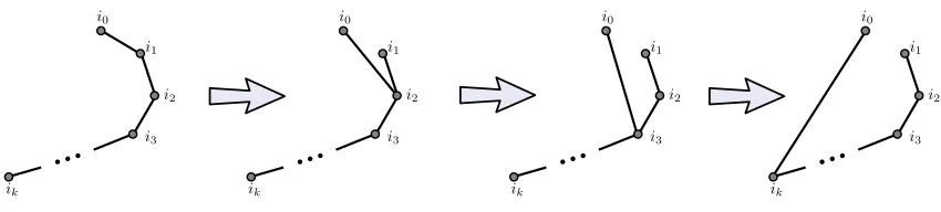
Using the sliding lemma iteratively on a pathp:=i0→i1→ · · · →ikthat is made of entangled rank-1
projectorsΠi0,i1, . . .Πik−1,ik, we can transform the first projectorΠi0,i1 to a projectorΠi0,i2, and then to
Πi0,i3, and so on until we obtainΠi0,ik, as illustrated inFigure 3. Let us denote the underlying 2-qubit
state inΠi0,ik, by|slide(p)i, i. e.,
Πi0,ik:=|slide(p)ihslide(p)|.
Then we reach the following corollary.
Corollary 4.5. Given a path p:=i0→i1→ · · · →ik of entangled rank-1 projectorsΠi0,i1, . . . ,Πik−1,ik,
apply the sliding lemma iteratively to obtain|slide(p)ii0,ik. Then the ground space of
Πi0,i1+Πi1,i2+· · ·+Πik−1,ik
is equal to the ground space of
Πi1,i2+· · ·+Πik−1,ik+|slide(p)ihslide(p)|.
Moreover, if|αii0is propagated to|βiik along p, then it is also propagated directly by|slide(p)ihslide(p)|.
Procedure 5ProbePropagation(i)
Propagation(s0,G0,i,|0i).
ifthe propagation is successfulthens1:=s0,G1:=G0 else
Let jsuch that|s0(j)|>1
findtwo pathsp1andp2inG0fromito jsuch thatprop(s0,p1,|0i)6=prop(s0,p2,|0i) finda product state|α⊥i ⊗ |β⊥iin the two-dimensional subspace span|slide(p1)i,|slide(p2)i undoPropagation(s0,G0,i,|0i)
ParallelPropagation(j,|αi,j,|βi)
Lemma 4.6. LetProbePropagationbe called when s0is closed, Hs0 has only rank-1entangled constraints,
G0=Gs0,s1=s0and G1=G0. Let s
0
0,s
0
1,G
0
0,G
0
1be the outcome of the procedure. Then the following holds:
1. IfProbePropagationdoes not output “H is unsatisfiable” then s00is a proper closed extension of s0, G00=Gs00,s01=s00and G01=G00. Moreover, if s is a pre-solution then s00is a pre-solution.
2. If the call toParallelPropagationoutputs “H is unsatisfiable” then H is unsatisfiable.
3. The complexity of the procedure is O(|Es0| − |Es00|).
Proof. If the procedure does not output “His unsatisfiable” then eitherPropagation(s0,G0,i,|0i)or one
of the parallel propagations (sayPropagation(s0,G0,i,|αi)) terminates successfully. Thuss00is a proper
extension ofs0becauses0is closed and therefores0(i) =. Obviouslys10 =s00 andG01=G00, and all
other claims follow from the Propagation Lemma.
Let us suppose that all three propagations are unsuccessful. ByCorollary 4.5, any solution forHs0
also satisfies the system obtained after sliding the constraints fromialong paths p1and p2, with the new
constraints|slide(p1)ihslide(p1)|i j and|slide(p2)ihslide(p2)|i j. UsingProposition 2.3, as|α⊥ii⊗ |β⊥ij
lies in span|slide(p1)i,|slide(p2)i , any state orthogonal to the latter subspace will also be orthogonal to
the former. Hence, any solution forHs0 should also satisfy the product constraint|α
⊥ih
α⊥|i⊗ |β⊥ihβ⊥|j.
Then,Lemma 4.3implies thatHs0, and by extensionHis unsatisfiable if the call toParallelPropagation,
made to satisfy|α⊥ihα⊥|i⊗ |β⊥ihβ⊥|j, fails.
For the complexity analysis the interesting case is when the first propagation, that we call
Propagationfailure, is unsuccessful but one of the two parallel propagations is successful. Let us
call this successful onePropagationsuccess. The main observation here is that every propagating edge
inPropagationfailurewill also be propagating inPropagationsuccess, because byLemma 3.2entangled
edges always propagate. The pathsp1andp2can be found in time proportional to the size of the subgraph visited byPropagationfailure. Indeed, observe that the edges of the two paths, except the last edge of
one of the two, are edges in the tree created by the breadth first search underlyingPropagationfailure.
The way from a vertex to the root of the tree can be found by maintaining, for each vertex in the tree, a pointer towards its parent. The product state|αi ⊗ |βican be found in constant time byProposition 2.3.
4.5 Analysis of the algorithm
Proof ofTheorem 4.1. If H is frustration free then by Lemma 4.2 MaxRankRemoval outputs a pre-solutions0that satisfies every maximal rank constraint. By the Propagation Lemma, at the end of Phase 2, s0is additionally a closed solution. ByLemma 4.3ParallelPropagationoutputss0such thatHscontains
only entangled constraints. ByLemma 4.6at the end of the algorithmHsis now empty, and thereforesis a solution.
If the algorithm does not output “His unsatisfiable” then byLemma 4.2, by the Propagation Lemma, and byLemma 4.3and Lemma 4.6it outputs an assignments such thatGs is the empty graph, and thereforesis a solution.
The complexity ofMaxRankRemovalbyLemma 4.2isO(|E|). After the second phase, the propa-gation of the assigned values duringMaxRankRemoval, the copying ofs0andG0into respectivelys1
andG1can be done by executing the same propagation steps this time withs1andG1. The complexity
of the rest of the algorithm by the Propagation Lemma,Lemma 4.3andLemma 4.6is a telescopic sum. Observe that the constants hidden in the big-O notation in the terms of this sum are all the same, they are equal to the absolute constant in the complexity analysis of the algorithmPropagationreferenced in the Propagation Lemma. Therefore the telescopic sum evaluates toO(|E|), and the overall complexity of the algorithm isO(|E|).
5
Bit complexity of
Q2SATSolver
As mentioned in the introduction, the algorithmQ2SATSolverhas been analyzed in the algebraic model of computation, where arithmetic operations on complex numbers are assumed to consume unit time. This was done mainly in order to simplify the presentation. However, in order to assess the running time of the algorithm in any realistic scenario, we must also take into account the actual cost of the arithmetic operations. This is not a completely trivial task: on the one hand, the continuous nature of a Q2SAT Hamiltonian implies that it should be represented using complex numbers with an exponentially high accuracy. But on the other hand, we also want the representation to be as efficient as possible, in order to minimize the total cost of each arithmetic operation. One way to approach this problem is to consider the input in the framework ofbounded algebraic numbersand analyze the complexity of the algorithm in this setting. Essentially, this would require calculating the bit-wise cost of representing the input in this framework and performing the arithmetic operations of the algorithm on it. In other words, we need to calculate thebit complexityof the algorithm. The techniques used in this section are based on standard methods in algebraic computational complexity, and further details can be found in [6].
Representing the input and the output
Definition 5.1(kQ-number). A rational numberuis akQ-number if there exists integersu1andu2of at
mostk-bits such thatu=u1/u2.
AkQ-numberu1/u2will be represented as the tuple(u1,u2)requiring 2kbits. As quantum projectors
and states use complex entries, we also require numbers fromQ(i), the extension field ofQwith i=
√ −1. This leads to the following definition of akQ(i)-number:
Definition 5.2(kQ(i)-number). A complex numbera+bi∈Q(i)is akQ(i)-number if its coefficientsa andbarekQ-numbers.
Ak
Q(i)-numbera+bi will be represented as the tuple(a,b)forkQ-numbersaandb, thereby requiring 4kbits in total. When the square root,√t, of a square-free integert(that is, an integer which is divisible by no perfect square other than 1) is generated during the course of the algorithm, we shall consider the field extensionQ(i,
√
t)ofQ(i)and the correspondingkQ(i,√t)-numbers, defined below.
Definition 5.3(k
Q(i, √
t)-number). The numbera1+a2
√
t+a3i+a4
√
ti∈Q(i,√t)is ak
Q(i, √
t)-number if its coefficients,a1,a2,a3anda4, arekQ-numbers.
Clearly, when the integertcan be represented as ak0-bit integer, ak
Q(i, √
t)-number can be represented using 8k+k0bits by the tuple(a1,a2,a3,a4,t)forkQ-numbersa1,a2,a3,a4.
The input Hamiltonian is a set ofmdifferent 2-qubit projectors whose non-trivial parts are 4×4 complex matrices. As mentioned inSection 2.2, for a 2-qubit projectorΠ=Πˆ ⊗Irest, the input specifies
the non-trivial part ˆΠwhich is uniquely determined by its image subspace,img(Πˆ). We consider each projector is given as akQ(i)-projectorwhich is defined below for some constantk>0.
Definition 5.4(kQ(i)-projector). Consider a 2-qubit projector ˆΠof rank-rto be specified byrindependent, but not necessarily orthogonal, 4×1 vectors{v1, . . . ,vr}such thatimg(Πˆ) =span{v1, . . . ,vr}. ˆΠis a
kQ(i)-projector ifv1,v2, . . . ,vrare given in the standard basis withkQ(i)-number coefficients.
Then, the Hamiltonian can be represented bymdifferentkQ(i)-projectors, leading to a total space consumption of at mostm×4×4×1×4k=64mkbits. The ground state output will be a tensor product of single qubit and 2-qubit states which are length 2 and 4 complex vectors, respectively. Each entry of these vectors could belong toQ,Q(i)orQ(i,
√
t), for different square free integerst. We will show below that there can be at mostn different integerst, and that the state assigned to each variable consumes
O(n)bits. Recall fromSection 2.4that the algorithm proceeds by assigning un-normalized states without affecting its accuracy. We also suppose that the basis vectors describing the image subspace of an input projector need not be normalized.
Cost of arithmetic operations
A useful fact on the bit complexity of basic arithmetic operations that will be used repeatedly is stated below. LetM(k,k0)be the time required to multiply ak-bit integer with ak0-bit integer and letM(k) = M(k,k). The currently known most efficient algorithm for integer multiplication uses Fourier transforms boundingM(k) =klogk8Θ(log∗k) [13] where
Fact 5.5. Let a be a kQ-number and b a k0
Q-number. Adding, subtracting, multiplying or dividing a and
b can be performed in time O(M(k,k0)), and the result is an O(k+k0)Q-number.
Now we consider the bit complexity incurred during the course of theQ2SATSolveralgorithm.
Theorem 5.6. Let H be aQ2SATHamiltonian on n qubits consisting of m projectors with complex entries, each given as two kQ(i)-numbers, for some constant k>0. Then the bit complexity ofQ2SATSolver(H) is O((n+m)M(n)).
Proof. The straightforward approach is to calculate the bit complexity of each operation that manipulates the projectors and assignments. In the first phase ofMaxRankRemoval, the unique state satisfying each 2-qubit projector of rank-3 can be found using Gaussian elimination which for anO(1)-sized matrix is equivalent to a constant number of multiplications. UsingFact 5.5, the 2-qubit state found will hence be anO(k)Q(i)-number.
The second and third phases of the algorithm repeatedly propagate values across rank-1 constraints. The bit complexity of propagation is now analyzed. Given a product constraint |αihα| ⊗ |βihβ|, it requires finding|α⊥i and|β⊥iusing complex conjugates. Given an entangled constraint and a state
assigned to one end of the constraint, the propagated state can be found by solving a system of linear equations. Assuming the initial state and the projector usekQ(i)-numbers, the propagated state will be represented using 2kQ(i)-numbers. To propagate`steps, each step usingkQ(i)-number projectors, starting with ak0
Q(i)-number state, the final propagated state will use(k
0+`k)
Q(i)-numbers. Hence, anO(n)step propagation will result in a final state represented withO(n)Q(i)-numbers whenk=O(1)andk0=O(n). This is linear in the number of qubits and takes at mostO(n)M(n,k)time. This covers the second and third phases of the algorithm.
The last phase withProbePropagationwill deal with one or more disconnected components, each made of only entangled constraints. The complexity of this phase is of interest when a contradiction arises during propagation in a component and a satisfying assignment has to be found by sliding constraints and usingProposition 2.3. Consider the way sliding across a constraint is done as described inLemma 4.4. Finding the transformation and its inverse both require a constant number of multiplications and the new constraint after sliding will be given using(ck)Q(i)-numbers for some constantc. Sliding alongO(n)
constraints will finally result in constraints represented byO(n)Q(i)-numbers and consumesO(n)M(n,k)
time.
Computing the product constraint in the resulting 2-dimensional subspace requires computing an eigenvector as per Proposition 2.3 leading to the possibility of an irrational square root √r being introduced into the representation, for some square-free integer r. This highlights the necessity of moving to the field extensionQ(i,
√
r). Assuming the two parallel rank-1 projectors were initially given usingk0
Q(i)-numbers, the product constraint will requireO(k
0)
Q(i,√r)-numbers to describe it. Also,
√
ris
generated as the irrational part of the eigenvalue of a 2×2 matrix whose entries areO(k0)Q(i)-numbers due to whichtwill be anO(k0)-bit integer. Hence, the representation of eachO(k0)
Q(i, √
t)-number will require
O(k0)bits. Any propagation after this point does not introduce new irrational square roots. The component, if satisfiable after`propagation steps, will have assignments given byO(k0+`k)
Q(i, √
t)-numbers. An
O(n)step propagation in this setting will result in this component usingO(n)
Q(i, √
Note that each disconnected component at the beginning of this phase may introduce different irrational square roots into their partial assignments.
Recall that since propagation is carried forward with unnormalised states, this is the only phase that may introduce square roots in the final assignment. The final output keeps all of these separate representations and does not homogenize them into a single representation. To conclude, each propagating, sliding or eigenvector finding step adds an overhead of at mostM(n,k)<M(n)where bit complexity is concerned. UsingTheorem 4.1, the bit complexity ofQ2SATSolveris thereforeO((n+m)M(n)).
Remark 5.7. The above explanation started by assuming the base representation field as that of the Gaussian rationals,Q(i), and extends to the appropriateQ(i,
√
r)field for some square-free integerr
when required. It is also possible to consider any algebraic number field as the base field and extend it appropriately using techniques from computational algebraic number theory [6]. Of course, any overheads in performing arithmetic operations and calculating field extensions will have to be accounted for accordingly.
References
[1] ITAI ARAD, MIKLOS SANTHA, AARTHI SUNDARAM, AND SHENGYU ZHANG: Linear time algorithm for quantum 2SAT. In Proc. 43rd Internat. Colloq. on Automata, Languages and Programming (ICALP’16), volume 55 of LIPIcs, pp. 15:1–15:14. Schloss Dagstuhl, 2016. [doi:10.4230/LIPIcs.ICALP.2016.15,arXiv:1508.06340] 1
[2] BENGTASPVALL, MICHAELF. PLASS,ANDROBERT ENDRETARJAN: A linear-time algorithm for testing the truth of certain quantified boolean formulas. Inf. Process. Lett., 8(3):121–123, 1979. [doi:10.1016/0020-0190(79)90002-4] 2
[3] NIEL DE BEAUDRAP AND SEVAG GHARIBIAN: A linear time algorithm for quantum 2-SAT. In Proc. 31st IEEE Conf. on Computational Complexity (CCC’16), volume 50 of LIPIcs, pp. 27:1–27:21. Schloss Dagstuhl, 2016. [doi:10.4230/LIPIcs.CCC.2016.27,arXiv:1508.07338] 5 [4] SERGEYBRAVYI: Efficient algorithm for a quantum analogue of 2-SAT. Contemporary
Mathemat-ics, 536:33–48, 2011. [doi:10.1090/conm/536,arXiv:quant-ph/0602108] 3,5
[5] JIANXINCHEN, XIE CHEN, RUANYAO DUAN, ZHENGFENGJI, AND BEI ZENG: No-go the-orem for one-way quantum computing on naturally occurring two-level systems. Phys. Rev. A, 83(5):050301, 2011. [doi:10.1103/PhysRevA.83.050301,arXiv:1004.3787] 8
[6] HENRICOHEN:A Course in Computational Algebraic Number Theory. Volume 138 ofGraduate Texts in Mathematics. Springer, 1993. [doi:10.1007/978-3-662-02945-9] 21,24
[7] STEPHEN A. COOK: The complexity of theorem-proving procedures. InProc. 3rd STOC, pp. 151–158. ACM Press, 1971. [doi:10.1145/800157.805047] 2
[9] MARTINDAVIS ANDHILARYPUTNAM: A computing procedure for quantification theory. J. ACM, 7(3):201–215, 1960. [doi:10.1145/321033.321034] 2,5
[10] JENSEISERT, MARCUSCRAMER,ANDMARTINB. PLENIO: Area laws for the entanglement en-tropy.Rev. Mod. Phys., 82(1):277–306, 2010. [doi:10.1103/RevModPhys.82.277,arXiv:0808.3773] 3
[11] SHIMON EVEN, ALONITAI,AND ADISHAMIR: On the complexity of timetable and multicom-modity flow problems. SIAM J. Comput., 5(4):691–703, 1976. Preliminary version inFOCS’75. [doi:10.1137/0205048] 2
[12] DAVID GOSSET AND DANIEL NAGAJ: Quantum 3-SAT is QMA1-complete. SIAM J. Com-put., 45(3):1080–1128, 2016. Preliminary version in FOCS’13. [doi:10.1137/140957056,
arXiv:1302.0290] 3
[13] DAVID HARVEY, JORIS VAN DER HOEVEN, AND GRÉGOIRE LECERF: Even faster integer multiplication. J. Complexity, 36:1–30, 2016. [doi:10.1016/j.jco.2016.03.001,arXiv:1407.3360] 22 [14] MICHAŁHORODECKI, PAWEŁ HORODECKI,ANDRYSZARDHORODECKI: Separability of mixed states: necessary and sufficient conditions. Phys. Lett. A, 223(1–2):1–8, 1996. [ doi:10.1016/S0375-9601(96)00706-2,arXiv:quant-ph/9605038] 6
[15] ZHENGFENGJI, ZHAOHUIWEI,ANDBEIZENG: Complete characterization of the ground-space structure of two-body frustration-free Hamiltonians for qubits. Phys. Rev. A, 84(4):042338, 2011. [doi:10.1103/PhysRevA.84.042338,arXiv:1010.2480] 4,18
[16] RICHARD M. KARP: Reducibility among combinatorial problems. InComplexity of Computer Computations, The IBM Research Symposia Series, pp. 85–103. Plenum Press, New York, 1972. [doi:10.1007/978-1-4684-2001-2_9] 2
[17] ALEXEIYU. KITAEV: Fault-tolerant quantum computation by anyons.Annals of Physics, 303(1):2– 30, 2003. [doi:10.1016/S0003-4916(02)00018-0,arXiv:quant-ph/9707021] 3
[18] ALEXEIYU. KITAEV, ALEXANDERSHEN,ANDMIKHAIL N. VYALYI:Classical and Quantum Computation. Amer. Math. Soc., 2002. [doi:10.1090/gsm/047] 3
[19] MELVENR. KROM: The decision problem for a class of first-order formulas in which all disjunctions are binary. Mathematical Logic Quarterly, 13(1–2):15–20, 1967. [doi:10.1002/malq.19670130104] 2
[20] CHRISTOPHERR. LAUMANN, RODERICHMOESSNER, ANTONELLOSCARDDICHIO,AND SHIV-AJIL. SONDHI: Random quantum satisfiability. Quantum Inf. Comput., 10(1):1–15, 2010. Link at
ACM DL. [arXiv:0903.1904] 5,11