Modelling infectious diseases with relapse: a case study of HSV-2

(1)

R E S E A R C H

Open Access

Modelling infectious diseases with

relapse: a case study of HSV-2

Jinliang Wang

1

, Xiaoqing Yu

1

, Heidi L. Tessmer

2

, Toshikazu Kuniya

3*

and Ryosuke Omori

2,4

*Correspondence: [email protected] 3_{Department of Applied} Mathematics, Graduate School of System Informatics, Kobe University, 1-1 Rokkodai-cho, Nada-ku, 657-8501 Kobe, Japan Full list of author information is available at the end of the article

Abstract

Background: Herpes Simplex Virus Type 2 (HSV-2) is one of the most common sexually transmitted diseases. Although there is still no licensed vaccine for HSV-2, a theoretical investigation of the potential effects of a vaccine is considered important and has recently been conducted by several researchers. Although compartmental mathematical models were considered for each special case in the previous studies, as yet there are few global stability results.

Results: In this paper, we formulate a multi-group SVIRI epidemic model for HSV-2, which enables us to consider the effects of vaccination, of waning vaccine immunity, and of infection relapse. Since the number of groups is arbitrary, our model can be applied to various structures such as risk, sex, and age group structures. For our model, we define the basic reproduction number0and prove that if0≤1, then the

disease-free equilibrium is globally asymptotically stable, whereas if0>1, then the

endemic equilibrium is so. Based on this global stability result, we estimate0for

HSV-2 by applying our model to the risk group structure and using US data from 2001 to 2014. Through sensitivity analysis, we find that0is approximately in the range of

2-3. Moreover, using the estimated parameters, we discuss the optimal vaccination strategy for the eradication of HSV-2.

Conclusions: Through discussion of the optimal vaccination strategy, we come to the following conclusions. (1) Improving vaccine efficacy is more effective than increasing the number of vaccines. (2) Although the transmission risk in female individuals is higher than that in male individuals, distributing the available vaccines almost equally between female and male individuals is more effective than concentrating them within the female population.

Keywords: Multi-group SVIRI epidemic model, Relapse, Basic reproduction number, Global asymptotic stability, Herpes Simplex Virus Type 2, Vaccination

Background

Herpes Simplex Virus Type 2 (HSV-2) is one of the most common sexually trans-mitted diseases, and has infected about 417 million people aged 15-49 worldwide [1]. Although there is still no licensed vaccine for HSV-2, a theoretical investigation of the potential effects of a vaccine is considered important and has recently been con-ducted by several researchers (see [2–4]). In [2, 3], compartmental epidemic models with vaccination for HSV-2 were considered and the effectiveness of the vaccina-tion was discussed in connecvaccina-tion with the basic reproducvaccina-tion number 0 (see [5])

(2)

through numerical simulations. However, there was little discussion about the stability of each equilibrium. As observed in several papers on epidemic models with vaccina-tion (see, for instance, [6–8]), backward bifurcavaccina-tion can occur at 0 = 1 for some special models and 0 < 1 does not necessarily imply the global asymptotic sta-bility of the disease-free equilibrium, that is, the eradication of the disease. In that case, the vaccination effort solely to make 0 < 1 has less significance. There-fore, a global stability analysis is critical for theoretically justifying the epidemiological discussion.

In [4], Lou et al. considered a compartmental epidemic model for HSV-2 with age and risk group structures and discussed the effectiveness of the vaccination together with the global stability analysis of each equilibrium. In their study, the vaccination was limited to female individuals, who are known to be the high-risk group for HSV-2, and it was concluded that such a vaccination strategy can reduce the total infections in both females and males. However, to support their conclusion, we need to consider a more general model in which male individuals can also benefit from the vaccina-tion and show that the optimal distribuvaccina-tion ratio of the vaccines is 1 to 0 for female and male individuals. In this paper, we consider such a general model and investi-gate the optimal distribution ratio of the vaccines. As opposed to their conclusion, our result shows that distributing the vaccines almost equally to females and males is more effective for the eradication of HSV-2 than concentrating them within the female population.

To consider the effect of vaccination with imperfect immunity, SVIR epidemic models are often formulated, in which the total population is subdivided into the suscepti-ble (S), vaccinated (V), infective (I) and recovered (R) populations (see, for instance, [2, 6–10]). However, to take into account the relapse of HSV-2 (see [2, 11]), it is necessary to also consider a direct transition from R to I. Thus, in this paper, we formulate a multi-group SVIRI epidemic model for HSV-2, which enables us to con-sider the effects of vaccination, of waning vaccine immunity, and of infection relapse. Since the number of groups is arbitrary, our model can be applied to various struc-tures such as risk, sex, and age group strucstruc-tures. In the empirical portion of this paper, we apply our model to the risk group structure and estimate the basic reproduc-tion number 0 for HSV-2 by using data from the US from 2001 to 2014. Since the infective population of HSV-2 seems to be in endemic equilibrium, the estimation of 0 must be carried out under the global asymptotic stability of the endemic equilib-rium. However, in general, the global asymptotic stability of the endemic equilibrium is not trivial.

(3)

estimated parameters, we discuss the optimal vaccination strategy for the eradication of HSV-2.

Methods

The general multi-group SVIRI epidemic model

Let n ∈ N be the number of groups and let N := {1, 2,· · ·,n}. Let Ni(t) be the

sexually active population in groupi ∈ N at timet. Let us divideNi(t)into four

sub-populations: susceptibleSi(t), vaccinatedVi(t), infectiveIi(t), and recoveredRi(t). Thus,

Ni(t)=Si(t)+Vi(t)+Ii(t)+Ri(t)for alli∈N. We make the following assumptions:

(A1) The number of individuals becoming sexually active in groupi ∈N per unit time isbi>0.

(A2) The per capita rate of removal from the sexual activity in groupi∈N isμi>0. (A3) The coefficient for disease transmission from infective individuals in groupj∈N

to uninfected (susceptible or vaccinated) individuals in groupi∈N isβij≥0. The

matrix(βij)i,j∈N is irreducible. The vaccine efficacy in groupi ∈ N isσi ∈[0, 1]

and the force of infection to vaccinated individuals in groupi∈ N is weakened by multiplyingσi. That is,

λS i(t):=

n

j=1 βij

Ij(t)

Nj(t)

and λV_i (t):=σi n

j=1 βij

Ij(t)

Nj(t)

, i∈N

are the forces of infection to susceptible and vaccinated individuals in groupi∈N at timet≥0, respectively. Here we assume standard incidence.

(A4) The per capita vaccination rate for susceptible individuals in groupi ∈ N isvi >

0. The per capita rate for the waning of vaccine-induced immunity for vaccinated individuals in groupi∈N isωi≥0.

(A5) The per capita recovery rate of infective individuals in groupi∈N isγi>0. (A6) The survival probability for recovered individuals in groupi∈N, who spent timet

in the recovered class, isPi(t):=exp(−

_t

0δi(η)dη), whereδi(η)denotes the relapse risk for individuals who spent timeη in the recovered class in groupi. For each i∈N,δi∈L1loc,+(0,+∞)and

+∞

0 δi(η)dη= +∞.

Under assumptions (A1)-(A2), we see that the time variation ofNi(t), i∈N is governed

by the following differential equation:

N_i(t)=bi−μiNi(t), i∈N. (1)

From the variation of constants formula, we easily see that limt→+∞Ni(t) = bi/μi =:

N_i∗, i ∈ N. Hence, without loss of generality, we can assume thatNi(t) ≡ Ni∗, i ∈ N.

Then, under assumptions (A1)-(A4), we obtain the differential equations forSi(t) and

Vi(t),i∈N as follows:

S_i(t)=bi−Si(t) n

j=1 βij

Ij(t)

N_j∗ −(μi+vi)Si(t)+ωiVi(t), (2)

V_i(t)=viSi(t)−σiVi(t) n

j=1 βij

Ij(t)

(4)

Under assumptions (A5)-(A6), the recovered population in groupi∈N at timetis given by

Ri(t)=

_+∞

0 γi

Ii(t−ξ)e−μiξe−

ξ

0δi(η)dη_dξ

=

t

−∞γiIi(ξ)e

−μi(t−ξ)_e−

t−ξ

0 δi(η)dη_dξ_, _i∈N_. ₍₄₎

By differentiating (4), we obtain the following integro-differential equation forRi(t),i∈N.

R_i(t)=γiIi(t)−μiRi(t)−

_t

−∞δi(t−ξ)γiIi(ξ)e

−μi(t−ξ)_e−

t−ξ

0 δi(η)dη_dξ

=γiIi(t)−μiRi(t)−

+∞

0 δi(ξ)γi

ξ

0δi(η)dη_dξ_. ₍₅₎

From (1)-(5) we obtain the integro-differential equation forIi(t),i∈N as follows.

I_i(t)=(Si(t)+σiVi(t)) n

j=1 βij

Ij(t)

N_j∗ −(μi+γi)Ii(t)

+

_+∞

0 δi(ξ)γi

_ξ

0 δi(η)dη_dξ_.

Under this setting, we arrive at the following main model in this paper. ⎧ ⎪ ⎪ ⎪ ⎪ ⎪ ⎪ ⎪ ⎪ ⎪ ⎪ ⎪ ⎪ ⎪ ⎪ ⎪ ⎪ ⎨ ⎪ ⎪ ⎪ ⎪ ⎪ ⎪ ⎪ ⎪ ⎪ ⎪ ⎪ ⎪ ⎪ ⎪ ⎪ ⎪ ⎩

S_i(t)=bi−Si(t) n

j=1 βij

Ij(t)

N_j∗ −(μi+vi)Si(t)+ωiVi(t),

V_i(t)=viSi(t)−σiVi(t) n

j=1 βij

Ij(t)

N_j∗ −(μi+ωi)Vi(t),

I_i(t)=(Si(t)+σiVi(t)) n

j=1 βij

Ij(t)

N_j∗ −(μi+γi)Ii(t)

+

+∞

0 δi(ξ)γi

ξ

0 δi(η)dη_dξ_, _i∈N_.

(6)

Note that the differential equation ofRi(t), i∈Ncan be omitted since it does not appear

in the above three equations.

The equilibria of system (6) can be obtained as the solution of the following algebraic equations. ⎧ ⎪ ⎪ ⎪ ⎪ ⎪ ⎪ ⎪ ⎨ ⎪ ⎪ ⎪ ⎪ ⎪ ⎪ ⎪ ⎩

0=bi−Si n

j=1 βij_NIj∗

j −(μi+vi)Si+ωiVi,

0=viSi−σiVi n

j=1βij Ij

Nj∗−(μi+ωi)Vi,

0=(Si+σiVi) n

j=1βij Ij

N_j∗ −(μi+γi−Qi)Ii, i∈N,

(7)

where

Qi:=

_+∞

0 δi(ξ)γi e−μiξ_e−

_ξ

0δi(η)dη_dξ_, _i∈N_.

Note that

Qi<γi

+∞

0 δi(ξ) e−

_ξ

0 δi(η)dη_dξ =γ i

−e−

_ζ

0 δi(η)dη+∞

(5)

It is easy to see that the trivial solution of (7) such thatIi = 0 for alli ∈ N always

exists. It is called the disease-free equilibrium of system (6) and we write it asE0 :=

S0₁,V₁0, 0,S0₂,V₂0, 0,· · ·,S0_n,V_n0, 0∈R3₊n, where

S0_i := bi

μi

μi+ωi μi+vi+ωi

, V_i0:= vi

μi+ωi

S_i0= bi μi

vi μi+vi+ωi

, i∈N.

Existence of the endemic equilibriumE∗ := S₁∗,V₁∗,I₁∗,· · ·,S_n∗,V_n∗,I_n∗ ∈ R3₊nsuch that I_i∗>0 for alli∈N will be discussed in connection with the basic reproduction number 0, which is defined as the expected number of secondary cases produced by a typical infected individual during its entire period of infectiousness at the initial invasion phase into a fully susceptible population, and given by the spectral radius of the next generation matrix (see [25]). Let

F:= ⎛ ⎜ ⎜ ⎝

S0₁+σ1v01

_β₁₁

N₁∗ · · ·

S0₁+σ1v01

_β₁_n

Nn∗

..

. . .. ...

S0_n+σnv0n

_β_n₁

N₁∗ · · ·

S0_n+σnv0n

_β_nn

Nn∗

⎞ ⎟ ⎟

⎠and V:=₁diag_≤_i_≤_n(μi+γi−Qi).

Then, according to [25], the next generation matrix is given by

K:=FV−1= ⎛ ⎜ ⎜ ⎜ ⎝

S0 1+σ1V10

β11

(μ1+γ1−Q1)N1∗ · · ·

S0 1+σ1V10

β1n

(μn+γn−Qn)Nn∗

..

. . .. ...

(S0n+σnVn0)βn1

(μ1+γ1−Q1)N1∗ · · ·

(Sn0+σnVn0)βnn

⎞ ⎟ ⎟ ⎟

⎠.

Hence, the basic reproduction number0is defined by

0:=ρ(K), (8)

where ρ(·) denotes the spectral radius of a matrix. We will obtain the global stability results for (6) in connection with0(see the “Results” section).

The special multi-group SVIRI epidemic model for HSV-2

The general model (6) can be applied to analyze the field data of HSV-2 epidemics. Sim-ilar to other sexually transmitted infections, the risk factor for HSV-2 infection is sexual behavior. To describe the heterogeneity of HSV-2 infection risk between host individu-als, we characterize the group as the combination of sex and their sexual behavior. We consider the following levels of sexual activity:x= 0, 1, 2,· · ·, 5 meaning the number of sexual partners within the last 12 months, wherex=5 implies the number of sexual part-ners is 5 or more. Lety∈ {1, 2}denote the sex, 1 denotes male and 2 denotes female. Then, the risk group is characterized byi ∈ {1, 2,· · ·, 12}in the following way:i = 2xi+yi,

where

(xi,yi)=

(m−1, 1) if i=2m−1,

(m−1, 2) if i=2m, m=1, 2,· · ·, 6.

For example,i= 2 corresponds to(xi,yi)= (0, 2)and implies the group of female

indi-viduals with no sexual partners andi = 11 corresponds to(xi,yi) = (5, 1)and implies

(6)

⎧ ⎪ ⎪ ⎪ ⎪ ⎪ ⎪ ⎪ ⎪ ⎪ ⎪ ⎪ ⎪ ⎪ ⎪ ⎪ ⎪ ⎪ ⎪ ⎪ ⎪ ⎨ ⎪ ⎪ ⎪ ⎪ ⎪ ⎪ ⎪ ⎪ ⎪ ⎪ ⎪ ⎪ ⎪ ⎪ ⎪ ⎪ ⎪ ⎪ ⎪ ⎪ ⎩

S_i(t)=bi−Si(t) 12

j=1 βij

Ij(t)

V_i(t)=viSi(t)−σiVi(t) 12

j=1 βij

Ij(t)

N_j∗ −(μi+ωi)Vi(t),

I_i(t)=(Si(t)+σiVi(t)) 12

j=1 βij

Ij(t)

N_j∗ −(μi+γi)Ii(t)

+

+∞

0 δi(ξ)γi

_ξ

0δi(η)dη_dξ_,

i∈ {1, 2,· · ·, 12}.

(9)

Note that (9) is a special case of (6). In this section, we assume thatδi(ξ)≡ δi>0 for all

i∈ {1, 2,· · ·, 12}. Note that the assumption (A6) is satisfied. In this case, we have:

_+∞

0 δi(ξ)γi

_ξ

0 δi(η)dη_dξ=δ i

_+∞

0 γi

Ii(t−ξ)e−μiξe−δiξdξ

=δiRi(t), i∈ {1, 2,· · ·, 12}.

Hence, together with the Eq. 5 ofRi(t), (9) can be simplified to the following multi-group

SVIRI epidemic model. ⎧ ⎪ ⎪ ⎪ ⎪ ⎪ ⎪ ⎪ ⎪ ⎪ ⎪ ⎪ ⎪ ⎪ ⎪ ⎪ ⎨ ⎪ ⎪ ⎪ ⎪ ⎪ ⎪ ⎪ ⎪ ⎪ ⎪ ⎪ ⎪ ⎪ ⎪ ⎪ ⎩

S_i(t)=bi−Si(t) 12

j=1 βij

Ij(t)

V_i(t)=viSi(t)−σiVi(t) 12

j=1 βij

Ij(t)

N_j∗ −(μi+ωi)Vi(t),

I_i(t)=(Si(t)+σiVi(t)) 12

j=1 βij

Ij(t)

N_j∗ −(μi+γi)Ii(t)+δiRi(t),

R_i(t)=γiIi(t)−(μi+δi)Ri(t), i∈ {1, 2,· · ·, 12}.

(10)

No vaccine against HSV-2 infection is currently available, so we ignore the vaccinated classVi,i∈ {1, 2,· · ·, 12}in the estimation of0. Then, (10) can be rewritten as follows.

⎧ ⎪ ⎪ ⎪ ⎪ ⎪ ⎪ ⎪ ⎪ ⎪ ⎨ ⎪ ⎪ ⎪ ⎪ ⎪ ⎪ ⎪ ⎪ ⎪ ⎩

S_i(t)=bi−Si(t) 12

j=1 βij

N_j∗Ij(t)−μiSi(t),

I_i(t)=Si(t) 12

j=1 βij

N_j∗Ij(t)−(μi+γi)Ii(t)+δiRi(t),

R_i(t)=γiIi(t)−(μi+δi)Ri(t), i∈ {1, 2,· · ·, 12}.

(11)

The basic reproduction number 0 for (11) is obtained as the spectral radius of the following matrix. ⎛ ⎜ ⎜ ⎜ ⎝ S0 1

μ1+γ1−Q1

β1,1 N₁∗ · · ·

S0 1

μ12+γ12−Q12

β1,12 N₁₂∗

..

. . .. ...

S0 12

μ1+γ1−Q1

β12,1 N₁∗ · · ·

S0 12

μ12+γ12−Q12

β12,12 N₁₂∗

⎞ ⎟ ⎟ ⎟

(7)

whereQi=δiγi/(μi+δi)and we writeβijasβi,jfor improved readability.

Transmission rates between the risk groupsiandj,βij, depend on sexual behavior and

sex. We modeledβijas follows;

βij=ρxiyiρxjyjRxixjSyiyj. (12)

The meaning of each symbol forβijis as follows.

• ρxiyidenotes the HSV-2 infection risk for the risk groupi. The risk group is stratified by sex and the number of partners within the last 12 months, the risk groupi denotes the individuals whose number of partners within the last 12 months isxiand sex isyi. ρxiyiis given by;

ρxiyi=cyi(xi+1)φ.

Here, similar to previous modelling studies of sexually transmitted infections, we modeled the relationship between infection risk and sexual behavior by a power law function [26].

• c denotes the sex specific HSV-2 transmission coefficient.

• φdenotes the exponent parameter describing the heterogeneity of the infection risk between different sexual behaviors.

• Rdenotes the mixing matrix between the risk groups defined by sexual behavior,x;

Rxixj =qδxixj +(1−q) y ρxyNxy

x yρxyNxy

.

This is the classical one-parameter ‘preferred mixing’ formulation, proposed by [27]. • δdenotes Kronecker’s delta.

• q denotes assortative coefficient. Whenq=0, the mixing between risk groups defined by sexual behavior is ‘proportionately mixing’, and the mixing is ‘fully assortative mixing’ whenq=1.

• Sdenotes the mixing matrix between sexes;

S=

a 1−a

1−a a

.

• a denotes the proportion of homosexual behavior.

We will use the special model (11) with transmission rate (12) to estimate the basic reproduction number0 for HSV-2 (see the “Results” section), and (10) with (12) to discuss the effectiveness of vaccination strategy (see the “Discussion” section).

Results

The main theorem

The main theorem of this paper is obtained for the general multi-group SVIRI epidemic model (6). Since (6) has an infinite time delay, we define the fading memory space (see, for instance, [28, 29]) as follows:

C:=φ ∈C((−∞, 0] ;R+):φ(s)esis uniformly continuous on(−∞, 0] , sup

s≤0|φ(

s)|es<+∞

(8)

whereis a positive constant such that 0< <mini∈N{μi}. Let us define the following

state space for system (6):

:=

ψ1,ψ2,· · ·,ψn,ψ˜1,ψ˜2,· · ·,ψ˜n,φ1(·),φ2(·),· · ·,φn(·)

∈R2n

+ ×Cn :

0< ψi<Si0, 0<ψ˜i <Vi0, φi(0) >0,

0< ψi+ ˜ψi+φi(0) <

bi μi

, i∈N

. (14)

The following proposition is proved:

Proposition 1is positively invariant for system(6).

The main theorem of this paper is as follows.

Theorem 1Let 0 and be defined by (8)and (14), respectively. Let ¯ denote the closure of.

(i) If 0 ≤ 1, then the disease-free equilibrium E0 ∈ ¯ of system (6) is globally asymptotically stable inand there exists no endemic equilibrium E∗in¯.

(ii) If0 >1, then the system(6)has the unique endemic equilibrium E∗inand it is globally asymptotically stable in.

For the proofs of Proposition 1 and Theorem 1, see the Appendix.

Theorem 1 still works for (10) since it is a special case of (6). In particular, although (10) does not include the integrated time delay, to our knowledge, there is no previous study on the global asymptotic stability of the endemic equilibrium of model (10). From this viewpoint, our main theorem can be regarded as valuable for the empirical study in the subsequent sections.

Estimation of0for HSV-2

Based on Theorem 1, we estimate the basic reproduction number 0 for HSV-2 in the US from 2001 to 2014. For the estimation of 0, we use the special model (11) with transmission rate (12). Note that (11) corresponds to the case where vi = σi = ωi = 0 for all i ∈ {1, 2,· · ·, 12}. Although the case where vi = 0 for

all i ∈ {1, 2,· · ·, 12} is excluded under assumption (A4), it is easy to check in a completely similar way as in the Appendix that the global stability result similar to Theorem 1 holds.

Previous study derived the value ofδiandγifrom empirical data,δiandγiare

param-eterized based on [30], 1/δi = 78.5 days and 1/γi = 13 days for alli ∈ {1, 2,· · ·, 12}.

Here note that we can regard μi as the removal rate from our system, which is given

by the sum of the sexual-inactivation rate and the mortality rate among those who are sexually active. We assume that the sexual life span is 50 years (15-65 years old) and parameterize the mortality rate by the national representative census data in the US [31], μi = 0.0231 per year for alli ∈ {1, 2,· · ·, 12}. Based on the previous

(9)

Table 1The model parameters and related estimates

Parameter Meaning Value Reference

δi(i=1, 2,· · ·, 12) Relapse risk 1/78.5 [30]

γi(i=1, 2,· · ·, 12) Recovery rate 1/13 [30]

μi(i=1, 2,· · ·, 12) Rate of removal from sexual activity 0.0231 [31]

q Assortative coefficient 0.3 [32]

a Proportion of homosexual behavior 0.02 [33] c1 Transmission coefficient for male 0.228 Estimated c2 Transmission coefficient for female 1.78 Estimated

φ Exponent parameter 0.700 Estimated

0 Basic reproduction number 2.07 Estimated

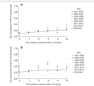
Using the observed data of sero-prevalence of HSV-2 in the US from 2001 to 2014 reported by [34], sex specific transmission coefficientcand the exponent parameterφ were estimated by maximum likelihood estimation. Since the antibody against HSV-2 infection (IgG) provides life-long immunity [35], we fittedI+Rto the observed data of the number of sero-positive cases for the estimation ofcandφ. To estimatecandφ, endemic equilibria ofIiandRiwere solved numerically with variedc1andc2andφ, and the set of c1andc2maximizing the likelihood function was explored. The likelihood function forc1 andc2is given by

L(c1,c2,φ)= Ti pmf

bin

N_idata_,_T , I

∗

i(ci,c2,φ)+R∗i(c1,c2,φ) N_i∗

,Pdata_i_,_T

.

Here pmf denotes the probability mass function, bin denotes a binomial distribution, N_idata_,_T denotes the observed data of the size of the risk groupiin sampling yearT, andPdata_i_,_T denotes the observed data of the number of HSV2-seropositive cases in the risk groupiin sampling yearT, respectively. For the confidence interval (CI) of the estimated parameter, profile likelihood-based confidence intervals were calculated. Using estimatedcandφthe basic reproduction number0for HSV-2 in the US was calculated. Figure 1 shows the comparison between the observed data of sero-prevalence of HSV-2 and the model esti-mates. The estimatedcare, transmission coefficient for male,c1 = 0.228 (95% CI 0.225 to 0.231), transmission coefficient for female,c2 =1.78 (95% CI 1.75 to 1.81), exponent parameterφ=0.700 (95% CI 0.693 to 0.707) and estimated0=2.07 (95% CI 2.03 to 2.11). Sexual behavior shows wide variation between host individuals. To assess the sensitivity of sexual behavior to0of HSV-2, we conducted a sensitivity analysis of the parameters describing sexual behavior, i.e., the proportion of homosexual partnershipaand assorta-tivity coefficient for the mixing between risk groupsq. Fig. 2 shows the relation ofaandq to estimated0,0increase if i)aincreases, and ii)qdecreases. The realistic variations ofaandq[36, 37] can induce the variation of0, which is approximately demonstrated in the range of 2-3.

Discussion

(10)

1.0

0.8

0.4

0.2

0.0 0.6

0 1 2 3 4 5+

The number of partner within 12 months

Sero-prevalence of HSV

-2 among male

1.0

0.8

0.4

0.2

0.0 0.6

Sero-prevalence of HSV

-2 among female

The number of partner within 12 months

0 1 2 3 4 5+

a

b

2001-2002 2003-2004 2005-2006 2007-2008 2009-2010 2011-2012 2013-2014

Year Year

Estimate

Fig. 1Comparison between the observed data of sero-prevalence of HSV-2 and the model estimates

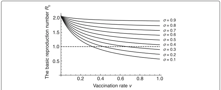
susceptible populationvand the vaccination efficacyσ. Here we have assumed that vac-cination is conducted with the same ratevfor the susceptible population over time. For simplicity, we assume that the efficacy of vaccineσis the same for all risk groups.

We first consider the case that vaccination rate v is the same between males and females. In this case, the basic reproduction number0with differentσ whenvvaries over (0, 1) is shown in Fig. 3. We see from Fig. 3 that, ifσ is 0.3 or smaller, 0 can be less than 1. On the other hand, if σ is 0.4 or larger, 0 cannot be less than 1 for anyv ∈ (0, 1). This implies that decreasing σ is more important than increasing

5

4

3

2

1

The basic reproduction number

R0

The proportion of homo-sexual partnerships a

0.02 0.04 0.06 0.08

0.0 0.1 0.2 0.3 0.4 0.5

5

4

3

2

1

The basic reproduction number

R0

Assortativity coefficient q

a

b

(11)

Fig. 3The relation ofvto estimated0with differentσ

v to reduce the basic reproduction number 0. That is, improving the vaccine effi-cacy is more important for the eradication of HSV-2 than increasing the number of vaccines.

We next discuss the optimal sex ratio of the vaccinated population to control HSV-2. HSV-2 infection is observed among females more frequently than males, “opportunistic” vaccination can induce higher vaccination coverage among females than males. To assess the optimal sex ratio of the vaccination rate, we expand the vaccination ratevas follows;

v1=pv, v2=(1−p)v, v: total vaccination rate.

Herepdenotes the sex ratio of vaccination. Figure 4 shows the relationship betweenp,

σ and0, we assumedv=0.9 as the representative value. Interestingly, small or largep increases0. This implies that vaccination biased to females (smallp) or males (largep) can result in persistence of the disease. In particular, it is noteworthy that the curves in Fig. 4 are almost symmetric with respect topand the minimum is attained near the center p=0.5. This implies that vaccination distributed equally to females and males is optimal for the eradication of the disease even though the transmission coefficient for males is lower than that for females.

(12)

Conclusion

In this paper, we have formulated the multi-group SVIRI epidemic model (6), which enables us to consider the effects of vaccination, the waning of vaccine-induced immunity, and relapse. We have defined the basic reproduction number0and proved Theorem 1, which states that if 0 ≤ 1, then the disease-free equilibrium E0 is globally asymp-totically stable, whereas if0 > 1, then the endemic equilibrium E∗ is so. Based on Theorem 1, we have estimated the basic reproduction number 0 for HSV-2 as 2.07 (95% CI 2.03 to 2.11) by using US HSV-2 data from 2001 to 2014. Through the sen-sitivity analysis for uncertain parameters on sexual behavior, we have found that 0 is approximately in the range of 2-3. Furthermore, using sensitivity analysis for vacci-nation parameters, we have discussed the effectiveness of the vaccivacci-nation. As a result, we have come to the following conclusions. (1) Improving vaccine efficacy is more effective than increasing the number of vaccines. (2) Although the transmission risk in female individuals is higher than that in male individuals, distributing vaccines almost equally to females and males is more effective than concentrating them within the female population.

Appendix

Proof of Proposition 1

We first show the positivity of the solution of system (6). Suppose that there existt1>0 and i∗ ∈ N such thatSi(t) > 0 and Vi(t) > 0 for all t ∈[ 0,t1) and i ∈ N and min(Si∗(t1),Vi∗(t1)) = 0. By the variation of constants formula, we have from the first equation in the system (6) that

Si∗(t1)=Si∗(0)e−

t₁

0 nj=1βi∗jIj(s)/Nj∗+μi∗+vi∗

ds

+

t1

0 (

bi∗+ωi∗Vi∗(s))e−

t₁

s n

j=1βi∗jIj(u)/Nj∗+μi∗+vi∗

du

ds >0.

Hence,Vi∗(t1) = 0. However, by the variation of constants formula, we have from the second equation in the system (6) that

Vi∗(t)=Vi∗(0)e−

t₁

0

σi∗ nj=1βi∗jIj(s)/Nj∗+μi∗+ωi∗

ds

+

t1

0

vi∗Si∗(s)e−

t₁

s

σi∗ nj=1βi∗jIj(u)/Nj∗+μi∗+ωi∗

du

ds >0,

which is a contradiction. Hence, we see thatSi(t) > 0 andVi(t) > 0 for allt > 0 and

i∈N.

Suppose that there existt2>0 and˜i∈N such thatIi(t) >0 for allt∈[ 0,t2)andi∈N andI_˜_i(t2)=0. By the variation of constants formula, we have from the third equation in the system (6) that

Ii(t)=Ii(0)e−(μi+γi)t+

t

0 ⎛

⎝₍Si(s)+σiVi(s))

n

j=1 βij

Ij(s)

N_j∗ +hi(s) ⎞

⎠e−(μi+γi)(t−s)_d_s_,

(15)

wherehi(t):=

_+∞

0 δi(ξ)γiIi(t−ξ)e−μiξe−

ξ

0δi(η)dη_dξ_{. We see that}_h

i(t)≥0 for alli∈N

andt∈[0,t1). Hence, from (15), we haveI˜i(t2) >0, which is a contradiction. Hence, we

(13)

The boundedness of the solution of system (6) immediately follows from the fact that N_i(t)=bi−μiNi(t),S_i(t)≤bi−(μi+vi)Si(t)+ωiVi(t)andV_i(t)≤viSi(t)−(μi+ωi)Vi(t)

for allt>0 andi∈N. This completes the proof.

Proof of (i) of Theorem 1

We define the following matrix, which corresponds to the next generation matrix:

M0:=V−1F = ⎛ ⎜ ⎜ ⎜ ⎝

S0₁+σ1V10

β11

(μ1+γ1−Q1)N1∗ · · ·

S0₁+σ1V10

β1n

(μ1+γ1−Q1)Nn∗

..

. . .. ...

(Sn0+σnVn0)βn1

(μn+γn−Qn)N₁∗ · · ·

(S0n+σnVn0)βnn

⎞ ⎟ ⎟ ⎟

⎠. (16)

In fact, it is easy to see thatρ(M0)=ρ(K)= 0.

First we show that system (6) has no endemic equilibriumE∗ ∈ ¯. Let us define the following matrix-valued function onR2n_{, which is equal to}_M0_if₍_S

1,V1,· · ·,Sn,Vn) = (S0₁,V₁0,· · ·S0

n,Vn0):

M(S1,V1,· · ·,Sn,Vn):=

⎛ ⎜ ⎜ ⎝

(S1+σ1V1)β11

(μ1+γ1−Q1)N1∗ · · ·

(S1+σ1V1)β1n

(μ1+γ1−Q1)Nn∗

..

. . .. ...

(Sn+σnVn)βn1

(μn+γn−Qn)N₁∗ · · ·

(Sn+σnVn)βnn

⎞ ⎟ ⎟

⎠.

Suppose that (S1,· · ·,Sn) = (S01,· · ·,Sn0). Then, from assumptions (A1)-(A6), we see

that 0 < M(S1,V1,· · ·,Sn,Vn) < M0, where 0 denotes the zero matrix and the

inequality implies that it holds for each element and each of the two matrices are not equal. Then, since it follows from assumptions (A1)-(A6) that matricesM0 _and_M0₊ M(S1,V1,· · ·,Sn,Vn)are nonnegative and irreducible, we can apply the Perron-Frobenius

theorem (see [38, Corollary 2.1.5]) to obtain thatρ (M(S1,V1,· · ·,Sn,Vn)) < ρ(M0)≤1.

This implies that the equationM(S1,V1,· · ·,Sn,Vn) (I1,· · ·In)T = (I1,· · ·In)T has only

the trivial solution(I1,· · ·,In)T = 0, whereT denotes the transpose of a vector. This

implies thatE∗does not exist in¯.

Next we show the global asymptotic stability of E0_{. It follows from the} Perron-Frobenius theorem (see [38, Theorem 2.1.4]) that M0 _{has a strictly positive left} eigenvector (1,· · ·,n), i > 0, i ∈ N corresponding to the eigenvalue ρ(M0): (1,· · ·,n) ρ(M0) = (1,· · ·,n)M0. Letci := i/ (μi+γi−Qi), i ∈ N andJi(t) :=

+∞

t δi(ξ)γie−μiξe−

_ξ

0 δi(η)dη_dξ_, _i∈N _{and consider the following Lyapunov function.}

LDFE(I1,· · ·,In):= n

i=1 ci

Ii(t)+

+∞

0

Ji(ξ)Ii(t−ξ)dξ

.

From assumption (A6),Ji(t)≥0,i∈Nfor allt≥0 and hence,LDFE≥0 and the equality

holds if and only if(I1,· · ·,In)≡0. Note that

+∞

0

Ji(ξ)Ii(t−ξ)dξ

=

_+∞

0

Ji(ξ)∂

∂tIi(t−ξ)dξ = −

_+∞

0

Ji(ξ)∂

∂ξIi(t−ξ)dξ = −[Ji(ξ)Ii(t−ξ)]+∞₀ +

_+∞

0 ∂

∂ξJi(ξ)Ii(t−ξ)dξ =QiIi(t)−

+∞

0 δi(ξ)γi

ξ

(14)

Hence, the derivative ofLDFEgives

LDFE= n

i=1 ci

⎛

⎝₍Si+σiVi)

n

j=1 βij

Ij

N_j∗−(μi+γi−Qi)Ii ⎞ ⎠

=

n

i=1 i

⎛ ⎜ ⎜ ⎜ ⎝

(Si+σiVi) n

j=1 βijIj

(μi+γi−Qi)Nj∗

−Ii

⎞ ⎟ ⎟ ⎟ ⎠

=(1,· · ·,n)·(M(S1,V1,· · ·,Sn,Vn)−En)·(I1,· · ·,In)T

≤(1,· · ·,n)·

MS₁0,V₁0,· · ·,S_n0,V_n0−En

·(I1,· · ·,In)T

=ρ(M0)−1(1,· · ·,n)·(I1,· · ·,In)T ≤ 0, (17)

whereEndenotes then-dimensional unit matrix and·denotes the product of vectors. It

is easy to see that when0<1,L_DFE=0 holds if and only ifIi=0 for alli∈N, that is,

the solution is in the disease-free equilibriumE0. When0 =1, from the third equality in (17), we see thatL_DFE=0 implies

(1,· · ·,n)·M(S1,V1,· · ·,Sn,Vn)·(I1,· · ·,In)T

=(1,· · ·,n)·(I1,· · ·,In)T. (18)

Suppose that (S1,V1,· · ·,Sn,Vn) =

S0₁,V₁0,· · ·,S0 n,Vn0

. Then (1,· · ·,n) ·

M(S1,V1,· · ·,Sn,Vn) < (1,· · ·,n)·M0 = ρ(M0) (1,· · ·,n) = (1,· · ·,n). Hence,

(18) has only the trivial solution such thatIi=0 for alli∈N. This implies thatL_DFE=0

holds only in the disease-free equilibrium E0 ∈ ¯. Consequently, from the LaSalle’s invariance principle (see [39]), we can conclude that the disease-free equilibriumE0is globally asymptotically stable.

Proof of (ii) of Theorem 1

If 0 > 1, then (1,· · ·,n) ·

MS0₁,V₁0,· · ·,S0_n,V_n0−En

· (I1,· · ·,In)T =

ρ(M0)−1(1,· · ·,n)·(I1,· · ·,In)T > 0. Hence, we see from the third equality in

(17) that in a neighborhood ofS0₁,V₁0,· · ·,S0 n,Vn0

,L_DFE>0. This implies the instability of the disease-free equilibriumE0.

Since the disease-free equilibrium ofE0of system (6) is unstable if0>1, we see from the uniform persistence result of [40] and an argument as in the proof of Proposition 3.3 of [41] that system (6) is uniformly persistent. That is, there exists a positive constantc>0 such that for any initial value, it holds that lim inft→+∞Si(t) ≥c, lim inft→+∞Vi(t)≥c

and lim inft→+∞Ii(t) ≥ cfor all i ∈ N. Since the uniform persistence together with

(15)

componentsS₁∗,V₁∗,I₁∗,· · ·,S∗_n,V_n∗,I_n∗ofE∗satisfy the following equations.

bi=S∗i n

j=1 βij

I_j∗

N_j∗ +(μi+vi)S

∗

i −ωiVi∗, (19)

viS∗i =σi n

j=1 βij

I_j∗

N_j∗ +(μi+ωi)V

∗

i , (20)

(μi+γi−Qi)I∗i =(Si∗+σiVi∗) n

j=1 βij

I_j∗

N_j∗, i∈N. (21)

As in [14], we defineθij:=

S_i∗+σiVi∗

βijIj∗/Nj∗,i,j∈N and

:= ⎛ ⎜ ⎜ ⎜ ⎜ ⎜ ⎜ ⎜ ⎜ ⎝

j=1θ1j −θ21 · · · −θn1 −θ12

j=2

θ2j · · · −θn2

..

. ... . .. ... −θ1n −θ2n · · ·

j=n θnj

⎞ ⎟ ⎟ ⎟ ⎟ ⎟ ⎟ ⎟ ⎟ ⎠ .

Letϕ := (ϕ1,· · ·,ϕn)T be a basis of the solution space of linear systemϕ = 0. Then,

from [14, Lemma 2.1], we see that the dimension of the solution space is 1 andϕi > 0,

i∈N. In particular, from the form of matrix, the following equality holds.

n

j=1 θijϕi=

n

j=1

θjiϕj, i∈N. (22)

Using thisϕandH(x):=x−1−lnx≥H(1)=0, we consider the following Lyapunov functional to prove the global asymptotic stability ofE∗.

LEE(S1,V1,I1,· · ·,Sn,Vn,In):= n

i=1 ϕi

S∗_iH

Si

S∗_i

+V_i∗H

Vi

V_i∗

+I_i∗H

Ii

I∗_i

+

_+∞

0

Ji(ξ)Ii∗H

Ii(t−ξ)

I_i∗

dξ

.

In order to make this function well-defined, without loss of generality, we can restrict our attention to the solution such thatIi(s) = ϕi(s), i ∈ N on(−∞, 0], whereϕi(0) =

Ii(0)and 0 < mi < ϕi(s) < Mi < +∞, s ∈ (−∞, 0] , i ∈ N for positive constantsmi

andMi,i∈ N. Then, from the positive invariance of setand the uniform persistence

(16)

Using (19), we can calculate the derivative ofLEEas follows.

L EE=

n

i=1

ϕi 1−

S∗_i Si

bi−Si n

j=1 βij

Ij

N_j∗ −(μi+vi)Si+ωiVi

+

1− V

∗ i

Vi

viSi−σiVi n

j=1 βij

Ij

N_j∗−(μi+ωi)Vi

+

1− I

∗ i

Ii (

Si+σiVi) n

j=1 βij

Ij

N_j∗ −(μi+γi)Ii

+

+∞

0 δi(ξ)γi

_ξ

0δi(η)dη_dξ

+

+∞

0

Ji(ξ)Ii∗ ∂ ∂tH

Ii(t−ξ)

I_i∗ dξ = n

i=1

ϕi 1−

S∗_i Si

S∗_i

n

j=1 βij

I_j∗

N_j∗ +(μi+vi)S

∗

i −ωiVi∗−Si n

j=1 βij

Ij

N_j∗

−(μi+vi)Si+ωiVi

+

1− V

∗ i

Vi

Si

S∗_iviS

∗ i −σiVi

n

j=1 βij

Ij

N_j∗ −(μi+ωi)Vi

+

1− I

∗ i

Ii (

Si+σiVi) n

j=1 βij

Ij

N_j∗ −(μi+γi)Ii

+

_+∞

0 δi(ξ)γi

_ξ

0δi(η)dη_dξ

−

_+∞

0

Ji(ξ)Ii∗ ∂ ∂ξH

Ii(t−ξ)

I_i∗ dξ = n

i=1 ϕi

μiS∗i

2− S

∗ i

Si −

Si

S∗_i

+viS∗i

2−S

∗ i

Si −

SiVi∗

S∗_iVi

+μiVi∗

1− Vi

V_i∗

+ωiVi∗

−1+S

∗ i

Si +

Vi

V_i∗− S∗_iVi

SiV_i∗+

1− Vi V_i∗

+S∗_i

n

j=1 βij

I_j∗

N_j∗

1−S

∗ i

Si

+S∗_i +σiVi∗

n

j=1 βij

Ii

N_j∗ −(Si+σiVi)

n

j=1 βij

I_j∗

N_j∗ I_i∗Ij

IiI_j∗

+(μi+γi)Ii∗

1− Ii

I∗_i

+

1− Ii I_i∗

+∞

0 δi(ξ)γi

_ξ

0 δi(η)dη_dξ

−

_+∞

0

Ji(ξ)Ii∗ ∂ ∂ξH

Ii(t−ξ)

I∗_i

dξ

.

(23)

Now it follows from integration by parts that

_+∞

0

Ji(ξ)Ii∗ ∂ ∂ξH

Ii(t−ξ)

I_i∗

dξ

= −Ji(0)Ii∗H

Ii

I_i∗

+ +∞

0

δi(ξ)γie−μiξe−

ξ

0 δi(η)dη_I∗ iH

Ii(t−ξ)

I_i∗

dξ

= −Qi

Ii−Ii∗−Ii∗ln

Ii(t)

I_i∗

+

+∞

0 δi(ξ)γi e−μiξ_e−

_ξ

0 δi(η)dη

Ii(t−ξ)−Ii∗−Ii∗ln

Ii(t−ξ)

I_i∗

(17)

Hence, (23) can be calculated as follows:

LEE

=

n

i=1 ϕi

μiS∗i

2−S

∗ i

Si −

Si

S∗_i

+viSi∗

2−S

∗ i

Si −

SiVi∗

S∗_iVi

+μiVi∗

1− Vi

V_i∗

+ωiVi∗

S∗_i Si −

S_i∗Vi

SiV_i∗

+S∗_i

n

j=1 βij

I_j∗

N_j∗

1− S

∗ i

Si

+S∗_i +σiVi∗

n

j=1 βij

Ii

N_j∗

−(Si+σiVi) n

j=1 βij

I_j∗

N_j∗ I_i∗Ij

IiI_j∗+(μi+γi−

Qi)Ii∗

1− Ii

I_i∗

−QiIi∗ln

Ii

I_i∗

−I∗_i

_+∞

0 δi(ξ)γi

Ii(t−ξ)

Ii −

1−lnIi(t−ξ) I_i∗

e−μiξ_e−₀ξδi(η)dη_dξ

. (24)

From (21) and (22), we have

n

i=1

ϕi(μi+γi−Qi)Ii= n

i=1

ϕi(μi+γi−Qi)Ii∗

Ii

I_i∗

=

n

i=1 ϕi

S_i∗+σiVi∗

n

j=1 βij

I∗_j N_j∗

Ii

I∗_i

=

n

i=1 Ii

I_i∗

n

j=1 θijϕi=

n

i=1 Ii

I_i∗

n

j=1 θjiϕj=

n

i=1 n

j=1 θji

Ii

I_i∗ϕj

=

n

i=1 n

j=1 θij

Ij

I_j∗ϕi=

n

i=1 ϕi

n

j=1 θij

Ij

I∗_j =

n

i=1 ϕi

S_i∗+σiVi∗

n

j=1 βij

Ij

N_j∗. (25)

Hence, using (20), (21) and (25), we can calculate (24) as follows:

LEE= n

i=1 ϕi

μiS∗i

2−S

∗ i

Si −

Si

S_i∗

+μiVi∗

3−S

∗ i

Si −

SiVi∗

S∗_iVi −

Vi

V_i∗

+ωiVi∗

2− SiV

∗ i

S∗_iVi −

S∗_iVi

SiVi∗

+S∗_i

n

j=1 βij

I_j∗ N_j∗

2−S

∗ i

Si −

SiIi∗Ij

S_i∗IiIj∗

+σiVi∗ n

j=1 βij

I_j∗

N_j∗

3− S

∗ i

Si −

SiVi∗

S∗_iVi −

ViI∗_iIj

V_i∗IiIj∗

−QiIi∗ln

Ii

I_i∗+QiI

∗ i ln

Ii

I_i∗−I

∗ i

+∞

0 δi(ξ)γi H

Ii(t−ξ)

Ii

e−μiξ_e−

ξ

0δi(η)dη_dξ

.

(26)

Using the inequality of arithmetic and geometric means, we see that the first three terms in the right-hand side of (26) are non-positive and equal to zero if and only if(Si,Vi) =

(18)

right-hand side of (26) is non-positive. Hence, taking the maximum as in [10] and using the graph-theoretic approach as in [14], we can evaluate (26) as follows:

L EE≤

n

i=1 ϕi

n

j=1

S_i∗+σiVi∗

βij

I_j∗ N_j∗

×max

2− S

∗ i

Si −

SiIi∗Ij

S∗_iIiIj∗

, 3−S

∗ i

Si −

SiVi∗

S∗_iVi −

ViIi∗Ij

V_i∗IiIj∗

=

n

i=1 ϕi

n

j=1 θijmax

2−S

∗ i

Si −

SiI∗_iIj

S∗_iIiIj∗

, 3− S

∗ i

Si −

SiVi∗

S∗_iVi −

ViI_i∗Ij

V_i∗IiIj∗

=

G∈

w(G)

(i,j)∈A(CG)

max

2− S

∗ i

Si −

SiI_i∗Ij

S∗_iIiIj∗

, 3−S

∗ i

Si −

SiVi∗

S∗_iVi −

ViI_i∗Ij

V_i∗IiIj∗

, (27)

wheredenotes the set of all unicyclic graphs included in directed graphs with vertices {1, 2,· · ·,n},Gdenotes the unicyclic graph included in,w(G) denotes the weight of graphG,CGdenotes the unicycle included inGandA(CG) denotes the set of all arcs included in CG. For instance, for a unicycle CG : 1 → 2 → 1, we have A(CG) = {(1, 2),(2, 1)}and thus,

(i,j)∈A(CG)

max

2−S

∗ i

Si −

SiI_i∗Ij

S_i∗IiIj∗

, 3− S

∗ i

Si −

SiVi∗

S∗_iVi −

ViI∗_iIj

V_i∗IiIj∗

=max

2−S

∗

1 S1−

S1I₁∗I2 S∗₁I1I₂∗

, 3− S

∗

1 S1 −

V₁∗S1 V1S₁∗ −

V1I₁∗I2 V₁∗I1I₂∗

+max

2−S

∗

2 S2−

S2I2∗I1 S∗₂I2I1∗

, 3− S

∗

2 S2 −

V₂∗S2 V2S2∗

− V2I2∗I1 V₂∗I2I1∗

=max

4−S

∗

1 S1−

S1I1∗I2 S∗₁I1I2∗

−S2∗ S2−

S2I2∗I1 S∗₂I2I1∗ ,

5− S

∗

1 S1 −

S1I1∗I2 S∗₁I1I2∗

− S∗2 S2 −

V₂∗S2 V2S2∗

− V2I2∗I1 V₂∗I2I1∗ ,

5− S

∗

1 S1 −

V₁∗S1 V1S∗₁ −

V1I₁∗I2 V₁∗I1I₂∗ −

S₂∗ S2−

S2I₂∗I1 S∗₂I2I₁∗ ,

6− S

∗

1 S1 −

V₁∗S1 V1S∗1

− V1I1∗I2 V₁∗I1I2∗

−S2∗ S2−

V₂∗S2 V2S∗2

− V2I2∗I1 V₂∗I2I1∗

.

We see that all elements in the max in the last expression of the above formula are non positive because of the inequality of arithmetic and geometric means. Similarly, we can easily check that for all unicycles CGwith at mostnvertices, the second sum in the last expression of (27) are non-positive (see [10, Proof of Theorem 4.1]). Hence, L_EE is non-positive and it is easy to check that the equality L_EE = 0 holds if and only if

(S1,V1,I1,· · ·,Sn,Vn,In) =

S₁∗,V₁∗,I₁∗,· · ·,S∗_n,V_n∗,I∗_n. This implies, from the LaSalle’s invariance principle, that the endemic equilibriumE∗is globally asymptotically stable.

Acknowledgements

We would like to thank the editor and anonymous reviewers for their helpful comments to the earlier version of this paper. We would like to thank Dr. Akihiro Ishii for helpful discussions regarding the serological test for HSV-2.

Funding

(19)

Medical Research and Development, AMED. RO was supported by Grant-in-Aid for Young Scientists (B) of Japan Society for the Promotion of Science (No. 15K19217) and Precursory Research for Embryonic Science and Technology (PRESTO) grant number JPMJPR15E1 from Japan Science and Technology Agency (JST). The authors were supported by JSPS Bilateral Joint Research Project (Open Partnership).

Availability of data and materials

The data that support the findings of this study are available in the National Health and Nutrition Examination Survey, “http://www.cdc.gov/nchs/nhanes/”.

Authors’ contributions

JW and XY formulated the model. HT improved the whole manuscript. TK carried out the theoretical analysis of the model. RO carried out the epidemiological study including the estimation of0for HSV-2. All authors read and approved

the final manuscript.

Ethics approval and consent to participate

Not applicable.

Consent for publication

Not applicable.

Competing interests

The authors declare that they have no competing interests.

Publisher’s Note

Springer Nature remains neutral with regard to jurisdictional claims in published maps and institutional affiliations.

Author details

1_{School of Mathematical Science, Heilongjiang University, 150080 Harbin, People’s Republic of China.}2_{Division of}

Bioinformatics, Research Center for Zoonosis Control, Hokkaido University, Sapporo, 001-0020 Hokkaido, Japan.

3_{Department of Applied Mathematics, Graduate School of System Informatics, Kobe University, 1-1 Rokkodai-cho,}

Nada-ku, 657-8501 Kobe, Japan.4_{JST, PRESTO, 4-1-8 Honcho, Kawaguchi, 332-0012 Saitama, Japan.}

Received: 9 April 2017 Accepted: 28 June 2017

References

1. World Health Organization. Media centre: Herpes simlex virus. 2017. Available from: http://www.who.int/. Accessed 25 Jan 2017.

2. Alsallaq RA, Schiffer JT, Longini IM, Wald A, Corey L, Abu-Raddad LJ. Population level impact of an imperfect prophylactic HSV-2 vaccine. Sex Transm Dis. 2010;37:290–7.

3. Blower S. Modelling the genital herpes epidemic. Herpes. 2004;3:138A–146A.

4. Lou Y, Qesmi R, Wang Q, Steben M, Wu J, Hefferman JM. Epidemiological impact of a genital herpes type 2 vaccine for young females. PLoS ONE. 2012;7:e46027.

5. Diekmann O, Heesterbeek JAP, Metz JAJ. On the definition and the computation of the basic reproduction ratio Ro in models for infectious diseases in heterogeneous populations. J Math Biol. 1990;28:365–82.

6. Kribs-Zaleta CM, Velasco-Hernández JX. A simple vaccination model with multiple endemic states. Math Biosci. 2000;164:183–201.

7. Arino J, McCluskey CC, van den Driessche P. Global results for an epidemic model with vaccination that exhbits backward bifurcation. SIAM J Appl Math. 2003;64:260–76.

8. Alexander ME, Bowman C, Moghadas SM, Summers R, Gumel AB, Sahai BM. A vaccination model for transmission dynamics of influenza. SIAM J Appl Dynam Syst. 2004;4:503–24.

9. Liu X, Takeuchi Y, Iwami S. SVIR epidemic model with vaccination strategies. J Theoret Biol. 2008;253:1–11. 10. Kuniya T. Global stability of a multi-group SVIR epidemic model. Nonlinear Anal RWA. 2013;14:1135–43. 11. van den Driessche P, Zou X. Modeling relapse in infectious diseases. Math Biosci. 2007;207:89–103.

12. Lajmanovich A, Yorke JA. A deterministic model for gonorrhea in a nonhomogeneous population. Math Biosci. 1976;28:221–36.

13. Feng Z, Huang W, Castillo-Chavez C. Global behavior of a multi-group SIS epidemic model with age structure. J Diff Equat. 2005;218:292–324.

14. Guo H, Li MY, Shuai Z. Global stability of the endemic equilibrium of multigroup SIR epidemic models. Canada Appl Math Quart. 2006;14:259–84.

15. Li MY, Shuai Z, Wang C. Global stability of multi-group epidemic models with distributed delays. J Math Anal Appl. 2010;361:38–47.

16. Ding D, Ding X. Global stability of multi-group vaccination epidemic models with delays. Nonlinear Anal RWA. 2011;12:1991–7.

17. Kuniya T. Global stability analysis with a discretization appraoch for an age-structured multigroup SIR epidemic model. Nonlinear Anal RWA. 2011;12:2640–55.

18. Shu H, Fan D, Wei J. Global stability of multi-group SEIR epidemic models with distributed delays and nonlinear transmission. Nonlinear Anal RWA. 2012;13:1581–92.

19. Yuan C, Jiang D, O’Regan D, Agarwal RP. Stochastically asymptotically stability of the multi-group SEIR and SIR models with random perturbation. Commun Nonlinear Sci Numer Simulat. 2012;17:2501–16.

(20)

21. Wang Z, Fan X, Han Q. Global stability of deterministic and stochastic multigroup SEIQR models in computer network. Appl Math Model. 2013;37:8673–86.

22. Zhang L, Pang J, Wang J. Stability analysis of a multigroup epidemic model with general exposed distribution and nonlinear incidence rates. Abstr Appl Math. 2013. 2013(Article ID .354287).

23. Wang J, Liu X, Pang J, Hou D. Global dynamics of a multi-group epidemic model with general exposed distribution and relapse. Osaka J Math. 2015;52:117–38.

24. Wang J, Pang J, Liu X. Modelling diseases with relapse and nonlinear incidence of infection: a multi-group epidemic model. J Biol Dynam. 2015;8:99–116.

25. van den Driessche P, Watmough J. Reproduction numbers and sub-threshold endemic equilibria for compartmental models of disease transmission. Math Biosci. 2002;180:29–48.

26. Liljeros F, Edling CR, Amaral LAN, Stanly HE, Aberg Y. The web of human sexual contacts. Nature. 2001;411:907–8. 27. Jacquez JA, Simon CP, Koopman J, Sattenspiel L, Perry T. Modelling and analyzing HIV transmission: the effect of

contact patterns. Math Biosci. 1988;92:119–99.

28. Hino Y, Murakami S, Naito T. Functional differential equations with infinite delay. vol. 1473 of Lecture Notes in Mathematics. Berlin: Springer-Verlag Berlin Heidelberg; 1991.

29. Röst G, Wu J. SEIR epidemiological model with varying infectivity and infinite delay. Math Biosci Eng. 2008;5:389–402. 30. Abu-Raddad LJ, Schiffer JT, Ashley R, Mumtaz G, Alsallaw RA, Akala FA, et al. HSV-2 serology can be predictive of HIV epidemic potential and hidden sexual risk behavior in the Middle East and North Africa. Epidemics. 2010;2:173–82. 31. Kochanek KD, Murphy SL, Xu J, Tejada-Vera B. Deaths: Final data for 2014. Natl Vital Stat Rep. 2016;65:1–122. 32. Abu-Raddad LJ, Jr IML. No HIV stage is dominant in driving the HIV epidemic in sub-Saharan Africa. AIDS. 2008;22:

1055–61.

33. Mumtaz G, Hilmi N, McFarland W, Kaplan RL, Akala FA, Semini I, et al. Are HIV epidemics among men who have sex with men emerging in the Middle East and North Africa?: a systematic review and data synthesis. PLoS Med. 2011;8:e1000444.

34. The National Health and Nutrition Examination Survey (NHANES). 2016. Available from:http://www.cdc.gov/nchs/ nhanes/. Accessed 25 July 2016.

35. van Wagoner NJ, III EWH. Herpes diagnostic tests and their use. Curr Infect Dis Rep. 2012;14:175–84. 36. Garnett GP, Anderson RM. Contact tracing and the estimation of sexual mixing patterns: the epidemiology of

gonococcal infections. Sex Trans Dis. 1993;20:181–91.

37. Sell RL, Wells JA, Wypij D. The prevalence of homosexual behavior and attraction in the United States, the United Kingdom and France: Results of national population-based samples. Arch Sex Behav. 1995;24:235–48.

38. Berman A, Plemmons RJ. Nonnegative matrices in the mathematical sciences. New York: Academic Press; 1979. 39. LaSalle JP. The Stability of Dynamical Systems. Philadelphia: SIAM; 1976.

40. Freedman HI, Ruan S, Tang M. Uniform persistence and flows near a closed positively invariant set. J Dynam Diff Equat. 1994;6:583–600.

41. Li MY, Graef JR, Wang L, Karsai J. Global dynamics of a SEIR model with varying total population size. Math Biosci. 1999;160:191–213.

42. Bhatia NP, Szego GP. Dynamical systems: stability theory and applications. Springer-Verlag; 1967.

43. Smith HL, Waltman P. The Theory of the Chemostat: Dynamics of Microbial Competition. Cambridge: Cambridge University Press; 1995.

• We accept pre-submission inquiries

• Our selector tool helps you to find the most relevant journal

• We provide round the clock customer support

• Convenient online submission

• Thorough peer review

• Inclusion in PubMed and all major indexing services

• Maximum visibility for your research

Submit your manuscript at www.biomedcentral.com/submit