A Numerical Comparison of Three Procedures Used in Failure Model Discrimination

A Numerical Comparison of Three Procedures

Used in Failure Model Discrimination

Samir Kamel Ashour

Institute of Statistical Studies & Research, Cairo University [email protected]

Ahmed Mortada Hashish

College of Business and Economics Qassim University

[email protected]

Abstract

Three different selection procedures namely RML, S and F-procedure are reviewed with application to exponential, Weibull, Pareto, and Finite range models. Some inaccurate results were discovered in the article of Pandy et al. (1991), it will be illustrated and modified. A simulation study is developed to numerically compare between the three procedures by obtaining the probability of correct selection.

Keywords: Discrimination; RML Procedure; S-Procedure; F-Procedure; PCS.

1. Introduction

To model the time to failure data for estimating reliability, several families of probability distributions are commonly used. In this paper, two pairs of distributions are considered: firstly, the Weibull and exponential distributions; secondly, the finite range and Pareto distributions. The problem that we consider in this article may be described as follows:

Suppose that we have a complete random sample T T₁, ₂,...,T_n as a life time data on a parent random variable T with distribution function F . It is required to decide that F is a member of one of a set of separate families of distribution functions say F F1, 2,...,Fk ,

without specifying the actual values of all or some parameters of the model. Consequently, we require a selection rule for deciding which of these k families best fits the sample. Practically, if k 2, we would like to choose between the two hypotheses

0: , ,...,1 2 n

H t t t was sampled from F₁

Versus H₁: , ,...,t t_{1 2} t_n was sampled from F₂.

the asymptotic distributions of the RML statistic under null hypotheses in discriminating between generalized exponential and Weibull models and between generalized exponential and gamma models. Kundu et al. (2005) derived the asymptotic distributions of the RML statistic in discriminating between generalized exponential and log-normal models. In addition, S-procedure has been proposed by Quesenberry and Kent (1982) to choose among exponential, gamma, Weibull, and lognormal models. Also, Pandey et al.

(1991) derived F-procedure to choose between exponential and Weibull models; and between finite range and Pareto models.

The present paper deals exclusively with discrimination between exponential and Weibull distributions; and between finite range and Pareto distributions. Their densities are given in table I where  and



are the scale and shape parameters of each model respectively.

It is necessary to point out that the exponential and Weibull models are two important failure models used frequently in reliability. Since the exponential distribution is a special case of the Weibull distribution, then we need to develop a method to discriminate between them. In our case of study, the exponential model has only a scale parameter, but the Weibull model has a scale and a shape parameter. Thus, the Weibull model is more powerful to fit any data drawn from the exponential model in case of unknown Weibull shape parameter. In other words, it isn't useful to discriminate between exponential and Weibull models in case of unknown Weibull shape parameter.

The finite range and Pareto models have a common property that the domain of their random variables depends on the scale parameters. This common property makes discriminating between the two models so difficult, therefore many methods were developed to discriminate between them.

A comparison among different selection procedures is done numerically by obtaining probability of correct selection (PCS), which is defined as the probability that a selection procedure leads to select the correct distribution.

2. Ratio of Maximized Likelihoods (RML)-Procedure

Dumonceaux et al. (1973) proposed the ratio of the maximized likelihoods (RML) statistic, which is given by

 

 

 

 

1 1

2 2

ˆ max

ˆ max

L L

RML

L L

 

 

 

 

 

 

 

 

,

where L₁ and L₂ are the likelihood functions for F₁ and F₂ with vectors of parameters  and  respectively and ˆ and ˆ are vectors of the maximum likelihood estimators for the parameters. This formula can be modified easily to be on the form of

 

 

 

 

1

1 2

2

ˆ

ˆ ˆ

( )

ˆ

L

n RML n nL nL

L



  



 

 

   

 

 

.

models, where the acceptance or rejection of any hypothesis depends only on the value of the RML statistic. In practice, F₁ best fits data if the RML statistic is greater than one (equivalent to  0), otherwise F₂ best fits data.

To discriminate between exponential and Weibull models using RML-procedure, suppose that the unknown scale parameter of exponential distribution is denoted by _e. Also, the unknown scale and known shape parameters of the Weibull distribution are denoted by

w

 and *

w

 ; respectively. Pandey et al. (1991) obtained the following natural logarithm of the ratio of the maximized likelihoods

 









 

* * *

1

ˆ ˆ ₁ n

w w e w w i

i

n n n n n t

     



   



, (1)

where ˆe and ˆw are the maximum likelihood estimators of e and w , respectively.

Using equation (1) the exponential model is selected if  0, otherwise if  0 the Weibull model is selected.

To discriminate between the Finite range and Pareto models using RML-procedure, suppose that the unknown scale parameter and unknown shape parameter of finite range distribution are denoted by _fr and _fr respectively. Also, the unknown scale and unknown shape parameters of the Pareto probability distribution are denoted by _p and

p

 respectively. Pandey et al. (1991) obtained the following natural logarithm of the ratio of the maximized likelihoods

 

 





 

1

ˆ _{ˆ ˆ}

ˆ ˆ ˆ ˆ

ˆ

n fr

fr fr p p fr p i

i p

n n  n n n n t

      

 

  _{ }

 _ _ _  _ 

 



, (2)

where, ˆ_fr, ˆ_fr, ˆ_p, and ˆ_p are the maximum likelihood estimators of the parameters

fr

 , _fr, _p, and _p respectively. Using equation (2) the finite range model is selected if 0

  , otherwise if  0 the Pareto model is selected.

3. S-Procedure

Quesenberry and Kent (1982) used a selection procedure based on statistics that are invariant under scale transformations of the data for choosing between the hypotheses mentioned in section 1. They found that their statistic has the property of being independent of the actual values of the scale parameter. The proposed selection rule is to select a distribution family Fi by obtaining the S statistic for each family. The S statistic

is given by

1

1 2

( , ,..., ) n

i i n

t

S 



f  t t  t d .

If k 2; the distribution family of F₁ is selected when n S( ₁) n S( ₂), otherwise the

To discriminate between the exponential and Weibull models using S-procedure, Quesenberry and Kent (1982) obtained the natural logarithm of S statistic for the exponential distribution as





1 ( ) ( ) n e i i

n S n n n n t



 

   _{ }





,

and for the Weibull distribution as

  

_{* *}



 





*

1 1

( ) ( 1) 1 ( ) w

n n

w w w i i

i i

n S n n   n t n n n n t 

 

 

       _{ }

 





.

Thus the exponential model is selected if n S( e) n S( w), otherwise the Weibull model

is selected.

To discriminate between the Finite range and Pareto models using S-procedure, Pandey

et al. (1991) obtained the natural logarithm of S statistic for the Pareto distribution as

 





 

1

ˆ ˆ

( ) ( 1) ( ) 1

n

p p p i

i

n S n n  n n  n t



    



.

Pandey et al. (1991) gave the following incorrect formula of the logarithm of the S statistic of Finite range distribution at page 1379





 

1

ˆ

( ) ( 1) ( ) 1

n

fr fr i

i

n S n n n  n t



    



.

But the correct formula is

 





 

1

ˆ ˆ

( ) ( 1) ( ) 1

n

fr fr fr i

i

n S n n  n n  n t



    



.

That can be proved as follows:

Proof :-

Using the Finite range pdf given in table I

( ; , ) , 0, 0

fr

fr

fr fr fr fr fr

fr t

f t t

t            _{ }     

The joint pdf of t t₁, ,...,₂ t_n is

1

1 2

1

( , ,..., ) fr fr

n n fr

n n i

i fr

f t t t _ t 











the S statistic will be

1

1 2

( , ,..., ) n

fr fr n

t

S 



f  t t t  d

( 1) 1 1

6 1 0 fr fr fr fr n n n n fr i n i fr

S t d

1 1 1 0 fr fr fr fr n n n fr

fr n i

i fr

S t d

     _{ }     





1 1 ₀ fr fr fr fr n n n fr

fr n i

i fr fr S t n              _{ }  



1 1 fr fr fr n n n fr fr

fr n i

i fr fr S t n          



1 1 1 fr n n fr fr i i S t n      



,

then, the logarithm of S is

 





 

1

ˆ ˆ

( ) ( 1) ( ) 1

n

fr fr fr i

i

n S n n  n n  n t



    



.

which proves our formula.

Thus the Pareto model is selected if n S( _p) n S( _fr), otherwise the finite range model is selected.

4. F-Procedure

Pandey et al. (1991) proposed the F-procedure for choosing between the hypotheses mentioned in section 1. The distribution families F₁ and F₂ are fitted using the regression equation of the form

y  a bx ,

as follows:

Try to obtain a linear function in t , n t( ) or n n t( ( )) using the reliability function

( )

R t , the cumulative hazard rate function H t( ) or their logarithmic transformations. This linear function is equated by the right hand side of the regression equation, a bx , to define X as some function of failure time T (i.e. X ( )T ) and a and b are functions in parameters. As a result, values of dependent variable x x₁, ₂,...,x_n are

calculated from the sample observations t t₁, ,...,₂ t_n [hint: use x_i ( )t_i ]. After that, equating the left hand side, y , by the corresponding empirical estimation of the right hand side which is a function of R t( ) or H t( ). Then, calculate the corresponding

1, 2,..., n

y y y . Finally, the F-statistic is computed according to the following formula:

1

2 ( 2)

i

Q

Q n

 

 , (3)

where 2 1 1 2 2 1 n i i i n i i

x y nxy Q x nx    _       





and

2 2 1 1 ( ) n i i

Q y y Q



Practically, both F₁ and F₂ are fitted to the sample data by calculated F-statistics of ₁ and ₂ respectively. Then F-procedure is proposed as: select F_i if _i max( , _{1 2}),

1, 2

i  . Practically, distribution family of F₁ is selected when  ₁ ₂ otherwise distribution family of F₂ is selected.

To discriminate between exponential and Weibull models using F-procedure, Pandey et al. (1991) formulated their regression equation to get with exponential x_j t_j, and the



( )



j n

n j

y n R t n

n



 

  _{   }

 , and with Weibull xj  n t( )j , and



( )



j n

n j

y n H t n n

n

   

  _{  }

 

  for j 1,...,n. By using equation (3) to obtain e

and _w the exponential model is selected if _e _w , while the Weibull model is selected otherwise.

To discriminate between Finite range and Pareto models using F-procedure, Pandey et al.

(1991) formulated their regression equation to get with finite range x_j  n t( )_j , and



( )



j n

j

y n F t n

n

 

  _{ }

 , and with Pareto xj  n t( )j , and n( )

n j

y H t n

n



 

 _{   }

 

for j 1,...,n. By using equation (3) to obtain _fr and _p the finite range model is selected if _fr _p, while the Pareto model is selected otherwise.

5. A Numerical Comparison

In our case of study, we consider two sets of two pairs of failure models, exponential versus Weibull and Pareto versus Finite Range. To carry out comparison, programs used to calculate the probability of correct selection (PCS) for each of the three selection procedures. In comparison, we have two cases:

Case 1: Exponential versus Weibull Model

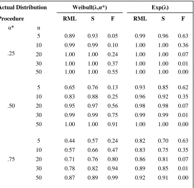
PCS values for exponential versus Weibull are computed and reported in table II. Numerical comparison in this case is carried out as follows:

When the data are coming from an exponential distribution, we consider

5,10, 20,30,50

But when the data are coming from a Weibull distribution, we consider

5,10, 20,30,50

n  and  .25,.5,.75,1.25,1.5,1.75, 2,5,10. Then, for different values of

n and  we generated a random sample of size n from Weibull distribution with shape parameter



and scale parameter  1 and check whether a given procedure correctly select the distribution or not. This process is replicated 10,000 times to obtain the PCS value for different values of n and



with each procedure. We notice that, when the data are drawn from a Weibull distribution, as the shape parameter



increases the PCS values for RML or S-procedure decrease until become near from  1 then switch to increase until reach the certainty with  greater than or equal 10. But in respect to F-procedure, we notice that its PCS values increase as



increases until reach the certainty with



greater than or equal 5.

Case 2: Finite Range versus Pareto Model

PCS values for finite range versus Pareto are computed and reported in table III. Similarly, numerical comparison in this case is carried out as follows:

When the data are coming from a Finite range distribution, we consider

5,10, 20,30,50

n  and  .25,.5,.75,1,1.25,1.5,1.75, 2,5,10. Then, for different values of n and  we generated a random sample of size n from Finite range distribution with shape parameter



and scale parameter 1 and check whether a given procedure correctly select the distribution or not. This process is replicated 10,000 times to obtain the PCS value for different values of n and  with each procedure. We notice that when the data are drawn from a Finite range distribution, as the shape parameter  increases the PCS values for RML or S or F-procedure remain constant.

But when the data are coming from a Pareto distribution, we consider n 5,10, 20,30,50

and .25,.5,.75,1,1.25,1.5,1.75, 2,5,10. Then, for different values of n and



we generated a random sample of size n from Pareto distribution with shape parameter



and scale parameter 1 and check whether a given procedure correctly select the distribution or not. This process is replicated 10,000 times to obtain the PCS value for different values of n and



with each procedure. We notice that when the data are drawn from a Pareto distribution, as the shape parameter



increases the PCS values for RML or S or F-procedure remain constant.

6. Notes on the Work of Pandey et al. (1991)

Pandey et al. (1991) carried out a numerical investigation to compute PCS values for the RML, S and F procedures in discriminating between exponential and Weibull models and between finite range and Pareto. They generated 5000 samples of size n 5,10 and 20

The problem which Pandey et al. (1991) faced were solved now. We could use a sample of size n 50 since the recent IBM machine has the ability to evaluate the gamma function ( )n for n 171. In addition, we generated 10,000 samples in all cases and that led to essentially different results. The reason behind choosing exactly 10,000 generated samples is the stationarity of results for the number of generated samples more than 10,000. On the other hand, Pandey et al. (1991) neither fixed the number of generated samples nor stated an acceptable reason behind generating varied number of samples changes from sample size to another.

7. Conclusions

Comparing RML with S with F-procedure in case of discriminating between exponential and Weibull models, we have the following two situations:

1. The actual distribution is exponential: using graph I when data are drawn from exponential, we notice that RML is more efficient for  1 while S is more efficient for 1  5, but for  5 the RML and S are equivalent.

2. The actual distribution is Weibull: using graph II when data are drawn from Weibull, we notice that S may be preferred to others procedures for  1 while RML may be preferred to others procedures for 1  5 but for  5 the RML, S and F are equivalent.

Similarly, comparing RML with S with F-procedure in case of discriminating between Finite range and Pareto models, we have the following two situations:

1. The actual distribution is Finite Range: using graph III when data are drawn from Finite Range, we notice that RML and F-procedure are preferred to S procedure for all



since they are equivalent.

2. The actual distribution is Pareto: When data are drawn from Pareto, we notice that RML is preferred to others procedures.

8. Appendix

Table I: Probability Densities functions used

Name Density

Exponential f t( )  1exp t  0, t 0.



  

 _ _  

 

Weibull

1

( ) t exp t , 0, 0.

f t t

 

 _{ }

  

 _{ }

   

 _{ } __{ } _  

  _   _

Finite range

1

( ) t 0, 0 .

f t t

t



 _{ }





 

 _{ }   

 

Pareto

1

( ) 0, .

f t t

t



  _{ }





 

 _{ }  

 

Table II: PCS of Exponential Distribution versus Weibull Distribution with unknown scale parameter 10,000 Generated Samples

Actual Distribution Weibull(λ,α*) Exp(λ)

Procedure RML S F RML S F

α* n

.25

5 0.89 0.93 0.05 0.99 0.96 0.63

10 0.99 0.99 0.10 1.00 1.00 0.36

20 1.00 1.00 0.24 1.00 1.00 0.07

30 1.00 1.00 0.37 1.00 1.00 0.01

50 1.00 1.00 0.55 1.00 1.00 0.00

.50

5 0.65 0.76 0.13 0.93 0.85 0.62

10 0.83 0.88 0.25 0.96 0.92 0.35

20 0.95 0.97 0.56 0.98 0.98 0.07

30 0.99 0.99 0.75 0.99 0.99 0.01

50 1.00 1.00 0.91 1.00 1.00 0.00

.75

5 0.44 0.57 0.24 0.82 0.70 0.63

10 0.57 0.66 0.47 0.83 0.75 0.35

20 0.71 0.76 0.80 0.86 0.81 0.07

30 0.78 0.82 0.94 0.89 0.85 0.01

50 0.87 0.89 0.99 0.92 0.91 0.00

1.25

5 0.80 0.67 0.50 0.40 0.54 0.62

10 0.79 0.71 0.79 0.52 0.61 0.36

20 0.82 0.76 0.98 0.65 0.71 0.06

30 0.83 0.79 1.00 0.71 0.76 0.01

50 0.88 0.86 1.00 0.80 0.83 0.00

1.50

5 0.86 0.75 0.62 0.50 0.63 0.62

10 0.88 0.82 0.89 0.66 0.74 0.35

20 0.92 0.89 1.00 0.81 0.85 0.06

30 0.95 0.92 1.00 0.88 0.90 0.01

50 0.97 0.97 1.00 0.95 0.96 0.00

1.75

5 0.90 0.81 0.71 0.57 0.69 0.62

10 0.92 0.88 0.94 0.76 0.83 0.36

20 0.97 0.95 1.00 0.90 0.92 0.06

30 0.99 0.98 1.00 0.95 0.97 0.01

50 1.00 0.99 1.00 0.99 0.99 0.00

2.00

5 0.93 0.85 0.79 0.64 0.75 0.63

10 0.95 0.92 0.97 0.83 0.88 0.36

20 0.99 0.98 1.00 0.96 0.97 0.07

30 0.99 0.99 1.00 0.98 0.99 0.01

50 1.00 1.00 1.00 1.00 1.00 0.00

5.00

5 0.99 0.98 1.00 0.93 0.96 0.63

10 1.00 1.00 1.00 1.00 1.00 0.35

20 1.00 1.00 1.00 1.00 1.00 0.06

30 1.00 1.00 1.00 1.00 1.00 0.01

50 1.00 1.00 1.00 1.00 1.00 0.00

10.00

5 1.00 1.00 1.00 0.99 0.99 0.63

10 1.00 1.00 1.00 1.00 1.00 0.35

20 1.00 1.00 1.00 1.00 1.00 0.06

30 1.00 1.00 1.00 1.00 1.00 0.01

Table II: PCS of Finite Range Distribution versus Pareto Distribution with unknown Shape and Scale parameters 10,000 Generated Samples

Actual Distribution Finite Range (λ,α) Pareto (λ,α)

Procedure RML S F RML S F

α n

.25

5 0.81 0.00 0.97 0.82 0.00 0.42

10 0.96 0.02 1.00 0.96 0.02 0.34

20 1.00 0.11 1.00 1.00 0.11 0.27

30 1.00 0.20 1.00 1.00 0.20 0.19

50 1.00 0.37 1.00 1.00 0.37 0.11

.50

5 0.81 0.00 0.98 0.81 0.00 0.43

10 0.96 0.02 1.00 0.96 0.02 0.35

20 1.00 0.11 1.00 1.00 0.11 0.25

30 1.00 0.20 1.00 1.00 0.20 0.20

50 1.00 0.36 1.00 1.00 0.36 0.12

.75

5 0.82 0.00 0.97 0.82 0.00 0.41

10 0.96 0.02 1.00 0.96 0.02 0.35

20 1.00 0.11 1.00 1.00 0.11 0.26

30 1.00 0.20 1.00 1.00 0.20 0.20

50 1.00 0.37 1.00 1.00 0.36 0.12

1.25

5 0.81 0.00 0.97 0.81 0.00 0.43

10 0.96 0.02 1.00 0.96 0.02 0.35

20 1.00 0.11 1.00 1.00 0.11 0.26

30 1.00 0.21 1.00 1.00 0.20 0.20

50 1.00 0.36 1.00 1.00 0.36 0.12

1.50

5 0.82 0.00 0.98 0.81 0.00 0.41

10 0.96 0.02 1.00 0.96 0.02 0.35

20 1.00 0.11 1.00 1.00 0.11 0.26

30 1.00 0.21 1.00 1.00 0.20 0.20

50 1.00 0.37 1.00 1.00 0.36 0.12

1.75

5 0.82 0.00 0.97 0.81 0.00 0.43

10 0.96 0.02 1.00 0.96 0.02 0.35

20 1.00 0.11 1.00 1.00 0.11 0.26

30 1.00 0.20 1.00 1.00 0.20 0.19

50 1.00 0.36 1.00 1.00 0.37 0.11

2.00

5 0.82 0.00 0.97 0.81 0.00 0.42

10 0.96 0.02 1.00 0.96 0.02 0.35

20 1.00 0.11 1.00 1.00 0.11 0.26

30 1.00 0.21 1.00 1.00 0.20 0.19

50 1.00 0.36 1.00 1.00 0.36 0.12

5.00

5 0.81 0.00 0.98 0.81 0.00 0.42

10 0.96 0.02 1.00 0.96 0.02 0.35

20 1.00 0.11 1.00 1.00 0.11 0.26

30 1.00 0.19 1.00 1.00 0.20 0.20

50 1.00 0.37 1.00 1.00 0.37 0.11

10.00

5 0.82 0.00 0.97 0.82 0.00 0.42

10 0.96 0.02 1.00 0.96 0.02 0.36

20 1.00 0.11 1.00 1.00 0.11 0.26

30 1.00 0.20 1.00 1.00 0.20 0.20

50 1.00 0.37 1.00 1.00 0.36 0.12

Table V: Overall Percentage of Correct Selection

Actual Distribution

Exponential Versus Weibull

Weibull(λ,α*) Exp(λ)

RML S F RML S F

91% 90% 78% 88% 89% 21%

Finite Range Versus Pareto

Finite Range(λ,α) Pareto(λ,α)

RML S F RML S F

95% 14% 99% 95% 14% 27%

9. References

1. Atkinson, A. C. (1970). A method for discriminating between models, Journal of the Royal Statistical Society, Ser. B, 32, 323-45.

3. Cox, D. R. (1961). Tests of separate families of hypotheses, Proc. 4th Berkeley Symp., 1, 105-123.

4. Cox, D. R. (1962). Further results on tests of separate families of hypotheses,

Journal of the Royal Statistical Society, Ser. B, 24, 406-424.

5. Dumonceaux, R. and Antle, C. (1973). Discrimination between the log-normal and the Weibull distributions, Technometrics, 5, 923-926.

6. Dumonceaux, R., Antle, C., and Haas, G. (1973). Likelihood ratio test for discrimination between two models with unknown location and scale parameters,

Technometrics, 15, 19-27.

7. Gupta, R. D. and Kundu, D. (2003). Discriminating between the Weibull and generalized exponential distributions, Comput. Statist. Data Anal., 43, 179-196. 8. Gupta, R. D. and Kundu, D. (2004). Discriminating between the gamma and

generalized exponential distributions, J. Statist. Comput. Simulation, 74(2), 107-121.

9. Jackson, O. A. Y. (1968). Some results on tests of separate families of hypotheses, Biometrika, 55, 2, 355-363.

10. Kundu, D., Gupta, R. D. and Manglick, A. (2005). Discriminating between the log-normal and generalized exponential distributions, Journal of the Statistical Planning and Inference, 127, 213-227.

11. Pandey, M., Ferdous, J. and Uddin, M. B. (1991). Selection of probability distributions for life testing data, Commun. Statist.-Theory Meth., 20(4), 1373-1388.