Random Intercept and Random Slope 2-Level Multilevel Models
Rehan Ahmad Khan
College of Statistical and Actuarial Sciences University of the Punjab Lahore, Pakistan [email protected]
Shahid Kamal
College of Statistical and Actuarial Sciences University of the Punjab Lahore, Pakistan [email protected]
Abstract
Random intercept model and random intercept & random slope model carrying two-levels of hierarchy in the population are presented and compared with the traditional regression approach. The impact of students’ satisfaction on their grade point average (GPA) was explored with and without controlling teachers influence. The variation at level-1 can be controlled by introducing the higher levels of hierarchy in the model. The fanny movement of the fitted lines proves variation of student grades around teachers.
Keywords: Random Intercept, Random Slope, Multilevel Models, Iterative Generalized Least Square.
1. Introduction
The contextual or group effects are common in social, educational and health sciences, for example, drug users use drugs mostly due to social imbalance in their lives, means factors at community or society level are influencing them to take drugs. The depression is greatly developed by social and environmental stressors. Early childhood development is strongly affected by many environmental conditions (nature of diet, impurity in the environment, care given by mother, amount of stimulation in the environment etc). The likelihood of teenagers in risky behavior is associated with frequently accompanying the adults company. On many occasions, people avoid divorce in our society due to social or religious constraints.
The common phenomena in all the examples stated above is the influence of group or upper level characteristics on the individual or lower level traits. So there exist a natural hierarchy in all the said problems (multilevel problems) and for the proper exploration, specialized analytical tools are required. Multilevel analytical tools provide the proper estimation of such type of problems.
problematic data set. As we study and collect the data at different natural stages of the population, we should use techniques, methods, tools that indulge the variation at each stage of the hierarchy i.e., use multilevel techniques.
A substantial advancement has been made both in methodological and applied divisions of the multilevel models due to its wide range of applicability in every field of science. Earlier development of methodology of multilevel model is based on Junior School Project (JSP) data (Goldstein, 1986, 1989, 1995, 1997, Longford, 1987, 1993 Mortimore et al., 1988, Woodhouse, 1995). Webster et al. (1996) identify school and teacher effects on student’s performance by using hierarchical linear models. Residential neighborhood has an effect on education (Benabou, 1993, Durlauf, 1996, Fernandez and Rogerson, 1997, Akerlof, 1997, Anselin, 2002). High school tracking characteristics such as selectivity, electivity, inclusiveness and scope on students have an effect on student performance (Gamoran, 1992). Extensive literature is available to study the application of multilevel models in education. Interested reader may see, Aitkin and Longford (1986), Nuttall et al. (1989), Willms (1992), Entwisle and Marton 1994), Gray et al. (1995), Goldstein and Spiegelhalter (1996), Roscigno (1998), Fielding (1999, 2004), Fraine et al. (2007, 2005). In this study, random intercept and random intercept & random slope two-level models are presented and compared with the traditional regression approach. The impact of students’ satisfaction on their grade point average (GPA) was explored with and without controlling teachers influence.
The basic simple linear regression model describing the relation of response variable y
and the explanatory variable x (both measured on level 1 of hierarchy) is defined as
0 1 (1.1)
y x
where, 0represents intercept and 1 is the slope of the line. Also the random term is
assumed to follow a normal distribution with mean 0 and constant variance 2. If the
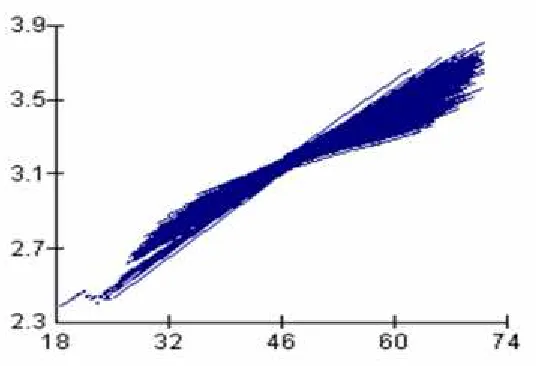
same variables y and x are measured for k groups and for each group regression line is fitted then we have k regression lines. Figure 1 is a display of such regression lines.
The fanny movement of the fitted lines suggests a variation of level-1 units across level-2 units. This means the characteristics measured at level-1 of hierarchy differ from level-2 unit to unit and if our attention is to consider the variation of all the variables measured at level 2 in a broader spectrum (population) then we need to build a single model accounting both level variables.
2. Random Intercept and Random Slope Model.
Let yijbe the ijth observation of a response variable y measured at level 1 and the
corresponding explanatory variable x observation xij ( j refers to level 2 unit and i
represents level 1 unit), then the basic simple linear regression model describing a simple linear relation between the response variable y and the explanatory variable x is,
0 1 1, 2,..., 1, 2,..., (2.1)
ij j j ij ij
y x i n j k
by fitting such k regression models we estimate 2k1 parameters, namely
2 0 1
( , )
j j j1,2,..., &k
e. Let 0j and 1j are the random variables as their magnitudevaries in k linear regression lines and assume that
0 0 0
1 1 1
(2.2) (2.3)
j j
j j
u u
where, u0jand u1j are the unexplained parts of ( , ) 0j 1j with parameters
2 2 2
0 1 0 0 1 1 0 1 01
( )j ( ) 0,var( )j j u ,var( )j u , cov( , )j j u
E u E u u
u
and u u
.The terms 0and1 are the average intercept and average slope of the k regression lines
respectively and the random variables u0j&u1j referred to as residuals are the random
departure of level-2 units from 0and1respectively. In addition, u0j N(0,
u20) and 21j (0, )u1
u N
. Also the residual term ij introduced at level-1 represents a randomvariation within level-1 units.
By considering (2.2) and (2.3), model (2.1) can be written as
0 0 1 1
0 1 0 1 (2.4)
ij j ij j ij ij
ij ij j j ij ij Fixed Part RandomPart
y u x u x
or
y x u u x
The presence of two residuals in the model separates it from the simple linear regression model (1) and for the estimation of the model we need to estimate two fixed parameters
0and 1
, and four random parameters 2 2 2
0, 1, 01 , 0
u u u and e
where
e20var( )
ij . Themodel (2.4) can also be described in matrices forms as:
(2.5)
where
1 1
11 1 12 2
2 2
21 1 22 2
1 1 2 2
1 1 2 2
(2.7)
j j k k
j j k k
ij j
i i ik k
nj j
n n nk k
e u e u
e u e u
e u e u
e u e u
e u
e u e u e u
e u
e u e u e u
R 1 1
11 12 1 2
2 2
21 22 1 2
1 2 1 2
1 2 1 2
(2.8)
j k j k
j k j k
ij j
i i ik k
nj j
n n nk k
e e u u
e e u u
e e u u
e e u u
e u
e e e u u u
e u
e e e u u u
R 1 (2.9)
2
R R R Where,
(1) (2)
1eij eij & 2 ej uj (2.10)
R R
also, the matrices of residuals have the following assumptions:
(2.11)( ) , ( ) (2.12)
( ) 0, (2.13)
T T T E E E E E 1 2
1 1 2(1) 2 2 2(2)
1 2 2 2(1) 2(2)
R R 0
R R V R R V
R R V V V
It is also assumed that the residuals at level-1 are independent to each other, so V2(1)is a
diagonal with ijthelement. Thus,
2 2
1 1 0
var( ) ij T , (2.14)
ij e e
e
2(1) j j
V X X
Similarly by assuming independence of residuals at level- 2, we gain V2(2) block diagonal
with jth elements
2
0 01 2 01 1
var( ) T , u u (2.15)
j
u u
u
2(2) j 2 j 2
V X Ω X Ω
11 11
21 21 0
1
1 1
, , (2.6)
1
k k
n k n k
y x y x y x
Y X τ
The jthblock of
2
V is therefore given by,
2 2
0 0 2
2(2) 2 2 0 0 0 (2.16) 0 ij u e
i e j
u e V (n) (n) 2j (n-1) (n-1) J I V V J I
where, I(n)is an (n n )identity matrix and J(n)is a (n n )matrix of ones. Furthermore,
is a direct sum operator.
The Generalized Least Square (GLS) estimates of τ can be obtained by using the relation:
-1
1 -1ˆ T T (2.17)
τ X V X X V Y
with variance-covariance matrix
X V XT -1
-1. For known τ one can estimate theresiduals as Y Y - Xτ E + E 1 2 with covariance matrix Y = YY* Tand E( )Y* V.
This is an iterative procedure by starting some reasonable estimates of fixed parameters and setting 2
0 0
u
. The estimates obtained from (2.17) are known as iterative generalized least square estimates as the procedure continues until the estimates converge (Goldstein, 1995).
Model (1.1) and (2.1) are estimated by using a real educational data collected by the researcher for PhD work. The data was collected from 40000 university students nested within 1000 university teachers. Students were considered as level-1 units and teachers as level-2. The response variable y was recorded as students grade point average score (GPA) and the explanatory variable x was student satisfaction with the university. Suppose we want to investigate whether the student grades vary from teacher to teacher and the impact of student satisfaction on their grades. We treat student satisfaction variable as a random variable across the teachers i.e., the coefficient of student satisfaction will vary across the teachers. We now assume a model which includes the possibility that the teachers have different slopes. This implies that the coefficient of explanatory variable will vary from teacher to teacher. Model (2.1) may be re-write by relating grade point average and student satisfaction (Stu_Sat) as,
0 1
0 0
1 1 1
_ (2.18)
(2.19) (2.20)
ij j j ij ij j oj
j j
GPA Stu Sat e
u u
20 0
2
1 01 1
2
0, : (2.21)
(0, ) (2.22)
j u
u
j u u
ij e u N u e N
Ωu
Now both the intercept and the slope vary randomly across teachers. Hence both the parameters 0j and 1j have a subscript j. Equation (2.19) describe that the intercept for
the jth teacher (0j) is given by0, the average intercept across all the teachers, plus a
random departure u0j. In the same way, equation (2.20) states that the slope for the jth
teacher (1j) is given by 1 , the average intercept across all the teachers, plus a random
departure u1j. The parameters 0 and 1 are the fixed intercept and slope of (2.18) and
jointly give the average line across all students nested in all teachers. The term u0jand
1j
u represent the random departures from 0and 1, or residuals at the teachers level i.e.,
they allow the jth teacher summary line to differ from the average line in both its slope and its intercept. The term u0jand u1jfollows a bivariate Normal distribution with mean
vector 0and covariance matrix Ωu. Here the covariance matrix Ωuis a 2 2 matrix
having 2 2
0, 1
u u
and u01its elements. The term u20 represents the variation in the
intercepts across the teachers summary line, 2 1
u
represent the variation in the slopes across the teachers summary line and the term u01shows the covariance between the
teachers intercepts and slopes. Finally, student’s grades depart from their teachers summary line by an amounteij, which is assumed to be normally distributed with mean 0
and variance 2
e
. Least square estimates of parameters under model 1.1 are available in table 1 and the iterative generalized least square estimates under model (2.18) are available in table 2.
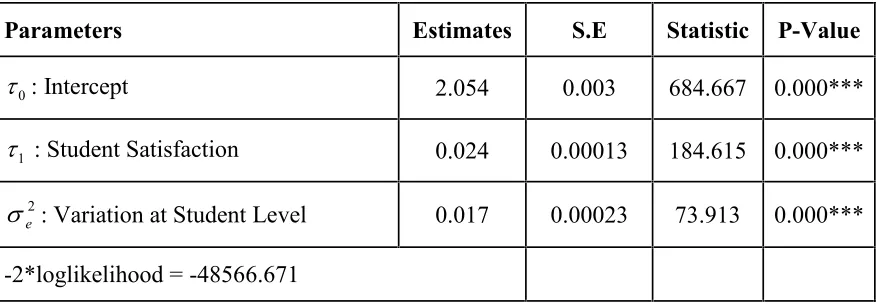
Table 1: Estimates of Parameters of Simple Linear Regression Model
Parameters Estimates S.E Statistic P-Value
0
: Intercept 2.054 0.003 684.667 0.000***
1
: Student Satisfaction 0.024 0.00013 184.615 0.000***
2
e
: Variation at Student Level 0.017 0.00023 73.913 0.000***-2*loglikelihood = -48566.671
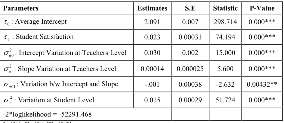
Table 2: Estimates of Parameters of Random Intercept and Random Slope Model
Parameters Estimates S.E Statistic P-Value
0
: Average Intercept 2.091 0.007 298.714 0.000***
1
: Student Satisfaction 0.023 0.00031 74.194 0.000***
2 0
u
: Intercept Variation at Teachers Level 0.030 0.002 15.000 0.000***
2 1
u
: Slope Variation at Teachers Level 0.00014 0.000025 5.600 0.000***
01
u
: Variation b/w Intercept and Slope -.001 0.00038 -2.632 0.00432**
2
e
: Variation at Student Level 0.015 0.00029 51.724 0.000***-2*loglikelihood = -52291.468
* p<0.05 ** p<0.01 *** p<0.001
The estimated coefficient of 1 is close to the estimate obtained from the model with a
simple slope. However, the individual teacher slopes vary about this mean with a estimated variance
0.00014( . 0.000025)
se
. The intercepts of the individual teacher lines also differ. Their mean is2.091( . 0.007)
se
and their variance is0.030( . 0.002)
se
. In addition, there is a negative covariance between intercepts andslopes estimated as
.001( . 0.00038)
se
suggesting that teachers with lower intercepts tend to have steeper slopes. This can also be confirmed with the correlation between intercepts and slopes across teachers estimated as 0.488. This negative correlation will lead to a fanning pattern of teachers lines. The variance for level-1 residuals (eij) is0.015 with standard error 0.00029 . The goodness of fit of a model may be explored through graphs of residuals and predicted values. The residuals estimated at any level can be used to test the assumption of normality i.e., at each level of hierarchy, it is assumed that the residuals should follow a normal distribution and this assumption may be checked by using a Normal probability plot, in which the ranked residuals are plotted against corresponding points on a Normal distribution curve and a straight line of points on a Normal plot indicate normality in residuals.
Graph 2(a). Normal Probability Plot
of Residuals at Level-1 Graph 2(b). Caterpillar Plot of Residuals atLevel-2 Graph 2(c). Normal Probability Plots ofResiduals at Level-2
Graph 2(d). Normal Probability Plot of Residuals Under Model 1.1
3. Random Intercept Model
Suppose we wish to examine the relationship between grade point average (response variable) and the teachers. The population is considered to have a two-level hierarchical structure with student’s grade point average (GPA) " "yij at 1 and teachers at
level-2. The random effect model with no explanatory variable can be described as,
2
0 ~ (0, ) (3.1)
ij j ij ij e
y e e N
2
0j 0 uoj u0j~ (0,N u0) (3.2)
from (3.2), (3.1) becomes,
0 (3.3)
ij ij oj y e u
Where eijand u0j are level-1 and level-2 residuals respectively. In this model u0j, the
teacher’s effect is assumed to be random variable having a normal distribution with variance 2
0
u
.
Model (3.1) is also known as variance components model because it partitions the residual variance into two components, level-2 variance (Between groups variance 2
0
u
) and level-1 variance (Within a group variance 2
e
Table 3: Estimated values of parameters of Random Intercept Model
Parameters Estimates S.E Statistic P-Value
0j
3.049 0.006 508.167 0.000***
2 0
u
0.030 0.001 30.0 0.000***
2
e
0.043 0.00023 186.96 0.000***
-2*loglikelihood = -9282.89
* p<0.05 ** p<0.01 *** p<0.001
The overall mean of GPA is estimated as ˆ0j 3.049. The means for the different
teachers are distributed about their overall mean with an estimated variance of 0.030. The variance among students within teachers is estimated as 2 0.043
e
and among teachers
variance is estimated as 2
0 0.030
u
. In order to test 2
0: u0 0
H (analogues to testing
0: 1 2 3... 1000 0
H in the fixed effect model), this variance appears significantly
different from zero (z30.0,p0.001).
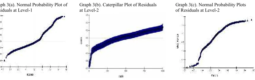
Graph 3(a) & 3(c) are normal probability plots of residuals at level-1 and level-2 respectively. Both graphs showed a fairly linear pattern of points indicating no worry about violation of normality assumption. In addition, points on graph 3(a) are linear as our response variable is normally distributed. Graph 3(c) is a caterpillar plot showing the residuals of 1000 level-2 units (teachers) with the 95% confidence intervals around them. Clearly, there is no considerable overlap of intervals indicating teachers have significant different means of student’s grades. These residuals also represent the departure of level-2 units (teachers) from the overall average predicted by the fixed parameter, this means that these are the teachers that differ significantly from the average at 5% level.
Graph 3(a). Normal Probability Plot of
Residuals at Level-1 Graph 3(b). Caterpillar Plot of Residualsat Level-2 Graph 3(c). Normal Probability Plotsof Residuals at Level-2
Discussion
variation may be controlled by introducing higher levels of hierarchy in the model. The reduction in the students’ grades variation under two-level model from the one-level model confirms the teachers influence over students grades.
The goodness of fit of model (3.1) may be tested through a compact test named likelihood ratio test. In a likelihood ratio test of 2
0: u0 0
H , we compare the model (3.1) with a model where 2
0
u
is constrained to equal to zero, i.e., the single level model with only an intercept term (y 0 e). The value of the likelihood ratio statistic is the
difference between the likelihood ratio of model (3.1) and the likelihood of the single level model (y 0 e) which is compared to a chi-squared distribution with 1 degree of
freedom i.e.,
2
8705.819 ( 9282.89) 17988.709
– 2
likelihood ratio of single level model likelihood ratio of level model
We conclude that there is a significant variation among teachers
2
( 17988.709,p0.001). The variance partition coefficient
2 0 2 2
0
0.030 0.411
0.030 0.043
u
u e
VPC
is showing 41%of the total variance in students grade point average is due to the differences among the teachers.
Similarly, model (1.1) is compared with a random slope model (2.1) and noticed that the value of 2*loglikelihood has decreased from
48566.671
to
52291.468
, a difference of 3724.797 . Since the model (2.1) involves two additional parameters, the variance of slope residuals 21
u
, and the covariance between intercepts and slopes u01, so
this difference follows a 2 distribution with
2 .
d f
. Under the null hypothesis thatthe extra parameters have population values of zero the change is highly significant, confirming the better fit of the model. In addition, about
65%(
VPC
0.653)
variation in students’ grades is due to the variation among teachers. Finally, it is concluded that a model may be predicted more efficiently by considering higher levels of hierarchy in a hierarchical population.References
1. Aitkin, M. and Longford, N. (1986). Statistical Modelling in School Effectiveness studies (with discussion).Journal of the Royal Statistical Society, A149, 1-43. 2. Akerlof, G.A. (1997). Social Distance and Social Decisions. Econometrica,
Econometric Society, 65, 5,1005-1028.
4. Bénabou, R. (1993). Workings of a City: Location, Education and Production.
Quavlerly Journal of Economics, 108, 619-652.
5. Bryk, A.S. and Raudenbush, S.W. (1992). Hierarchical Linear Models. Newbury Park, CA: Sage.
6. De Fraine, B., Van Damme, J., &Onghena, P. (2007). A Longitudinal analysis of gender differences in academic self-concept and language achievement: A multivariate latent growth curve approach. Contemporary Educational Psychology, 32, 132-150.
7. De Fraine, B., Van Landeghem, G., Van Damme, J., &Onghena, P. (2005). An analysis of well-being in secondary school with multilevel growth curve models and multilevel multivariate models.Quality and Quantity, 39, 297-316.
8. De Leeuw, J. and Kreft, Ita G.G. (1986). Random Coefficient Models. Journal of Educational Statistics, 11, 1, 55-85.
9. Durlauf, S.N. (1996). Statistical Mechanics Approaches to Socioeconomic Behavior.NBER Technical Working Papers 0203, National Bureau of Economic Research, Inc.
10. Entwistle, N.J. and Marton, F. (1994). Knowledge objects: understandings constituted through intensive academic study. British Journal of Educational Psychology, 64,161-78.
11. Fielding, M. (1999). Radical collegiality: Affirming teaching as an inclusive professional practice.Australian Educational Researcher, 26, 2, 1–34.
12. Fielding, M. (2004). Transformative approaches to student voice: Theoretical underpinnings, recalcitrant realities. British Educational Research Journal, 30, 2, 295–311.
13. Gelman, A. and Jennifer, H. (2007). Data Analysis Using Regression and Multilevel/Hierarchical Models. New York: Cambridge University Press.
14. Goldstein, H. (1986). Multilevel mixed linear model analysis using iterative generalised least squares. Biometrika, 73, 43-56.
15. Goldstein, H. (1989a). Restricted unbiased iterative generalised least squares estimation.Biometrika, 76, 622-623.
16. Goldstein, H. (1995). Multilevel Statistical Models, 2nd edition. London, Edward Arnold: New York, Wiley.
17. Goldstein, H. (2003). Multilevel Statistical Models, 3rd edition. London, Edward Arnold: New York, Wiley.
18. Goldstein, H. (1997). Methods in school effectiveness research. School Effectiveness and School Improvement, 8, 369-395.
19. Goldstein, H. and Spiegelhalter, D.J. (1996). League tables and their limitations: statistical issues in comparisons of institutional performance.Journal of the Royal Statistical Society, A159, 505-513.
20. Gray, J., Jesson, D., Goldstein, H., Hedger, K. and Rasbash, J. (1995). A multi-level analysis of school improvement: Changes in school performance over time.
21. Longford, N.T. (1987). A fast scoring algorithm for maximum likelihood estimation in unbalanced mixed models with nested random effects. Biometrika, 74, 817-827.
22. Longford, N.T. (1993).Random Coefficient Models. Oxford: Clarendon Press. 23. Mortimore, P., Sammons, P., Stoll, L., Lewis, D. and Ecob, R. (1988). School
Matters. Wells, Open Books.
24. Nuttall, D.L., Goldstein, H., Prosser, R. and Rasbash, J. (1989). Differential school effectiveness.International Journal of Educational Research, 13, 769-776. 25. Raudenbush, S.W. and Bryk, A.S. (1986). A hierarchical model for studying
school effects.Sociology of Education, 12, 241-269.
26. Raudenbush, S.W. and Bryk, A.S. (2002). Hierarchical Linear Models: Applications and Data Analysis Methods. 2nd ed. Newbury Park, CA: Sage. 27. Reise, S.P. and Duan, N. (2003).Multilevel Modeling: Methodological Advances,
Issues, and Applications. Lawrence Erlbaum Associate, Inc.
28. Roscigno, V.J. (1998). Race and Reproduction of Educational Disadvantages.Social Forces,76, 1033-1060.
29. Skrondal, A. and Hesketh, S.R. (2004). Generalized Latent Variable Models: Multilevel, longitudinal, and structural equation models. Boca Raton: Chapman & Hall.
30. Smith, R.B. (2011). Multilevel Modeling of Social Problems: A Causal Perspective. New York, Springer.
31. Snijders, T and Bosker, R. (1999).Multilevel Analysis. London, Sage.
32. Webster, W., Mendro, R., Orsak, T. and Weerasinghe, D. (1998). An application of hierarchical linear modeling to the estimation of school and teacher effect.
Paper presented at the Annual Meeting of the American Educational Research Association, San Diego, CA, April 13-17.
33. Willms, J.D. (1992). Monitoring school performance: A guide for educators. Lewes: Falmer Press.