Cluster Size and Aggregated Level 2
Variables in Multilevel Models.
A Cautionary Note
Reinhard Schunck
GESIS – Leibniz Institute for the Social Sciences
Abstract
This paper explores the consequences of small cluster size for parameter estimation in mul-tilevel models. In particular, the interest lies in parameter estimates (regression weights) in linear multilevel models of level 2 variables that are functions of level 1 variables, as for instance the cluster-mean of a certain property, e.g. the average income or the proportion of certain people in a neighborhood. To this end, a simulation study is used to determine the effect of varying cluster sizes and number of clusters. The results show that small cluster sizes can cause severe downward bias in estimated regression weights of aggregated level 2 variables. Bias does not decrease if the number of clusters (i.e. the level 2 units) increases.
Keywords: multilevel modeling, hierarchical linear model, sample size, survey research, cluster sampling
Direct correspondence to
Reinhard Schunck, GESIS – Leibniz Institute for the Social Sciences, Unter Sachsenhausen 6-8, 50667 Köln, Germany
E-Mail: [email protected]
Acknowledgements: I would like to thank Carsten Sauer and three anonymous reviewers for the helpful and critical comments.
1 Introduction
Multilevel models (also known as hierarchical linear models and mixed models) are a common statistical tool for the analysis of clustered data (De Leeuw, Meijer, & Goldstein, 2008; Langer, 2010; Rabe-Hesketh & Skrondal, 2012; Raudenbush & Bryk, 2002; Snijders & Bosker, 2012). Their advantages are obvious: instead of treating observations incorrectly as unrelated, they explicitly take the clustering of observations into account and allow for modeling how characteristics of the higher level impact units at the lower level – for example, how neighborhood characteris-tics affect residents or how school characterischaracteris-tics affect students.
It is common in multilevel modeling to aggregate level 1 information to gener-ate level 2 information, i.e. to characterize the clusters in which the lower level units are nested. For instance, the proportion of immigrant children in schools, the proportion of unemployed respondents in neighborhoods, the average income in neighborhoods and similar measures are frequently used in multilevel analysis (Fauth, Roth, & Brooks-Gunn, 2007; Gross & Kriwy, 2013; Pong & Hao, 2007; Schunck & Windzio, 2009; Windzio, 2004; Windzio & Teltemann, 2013).
In multilevel analysis cluster means are frequently assumed to have a meaning-ful interpretation, which is substantively different from the level 1 variables from which they are calculated. For instance, the mean household income in a neigh-borhood may be seen as a measure of neighneigh-borhood quality.1 This paper
investi-gates how level 1 sparseness, that is having few observations per cluster, affects the estimation of the regression weights of such aggregated level 2 variables in linear multilevel models.
Level 1 sparseness is not uncommon in empirical research. Research is often confronted with data that is of a hierarchical nature but contains only few observa-tions per cluster. This is common in surveys that follow stratified sampling designs, where only few respondents are clustered in geographical units (Clarke & Whea-ton, 2007; Schunck & Windzio, 2009).
Questions regarding adequate sample sizes at each level in multilevel analysis have been discussed before (Bell, Ferron, & Kromrey, 2008; Clarke, 2008; Clarke
& Wheaton, 2007; Hox, 1998; Kreft, 1996; Maas & Hox, 1999, 2005). Prior research suggests that level 1 sparseness does not lead to serious bias in parameter estimates (Bell et al., 2008; Clarke, 2008; Clarke & Wheaton, 2007; Maas & Hox, 2005). The number of clusters (level 2 units) seems to be more important than the number of observations per cluster. However, previous research has not systematically investi-gated how small sample sizes at level 1 impacts the estimates in multilevel models if these models include aggregated level 2 variables that are a function of the level 1 variables. In this case, small cluster size may cause noisy and unreliable aggrega-tions. This becomes obvious if we consider the reliability of aggregated variables in multilevel models. For an aggregated indicator the reliability of the group mean can be expressed by
(1)
where 2
B
σ is the between group-variance of the indicator, 2
W
σ is the within-group
variance, and ni is the common cluster size (Snijders & Bosker, 2004, pp. 25-26). Reliability increases if the number of level 1 units per cluster increases and reli-ability decreases when the number of observations per cluster decreases.2 In linear
models, low reliability will create an error-in-variables problem and will cause an attenuation bias (Wooldridge, 2010, p. 81). This study therefore considers the effects of very small cluster sizes in linear two-level multilevel models on parameter esti-mates of regression weights of level 2 variables that are a function of level 1 vari-ables.
2 Methods
To this end, this study uses Monte Carlo simulations, varying a) the cluster size, i.e. the number of level 1 units per cluster (ni = 5, 10, 20, 40, 80) and b) the number of
level 2 units (nj = 20, 40, 100, 1000). The number and size of clusters is chosen to include the range of cluster sizes and numbers of clusters typically encountered in multilevel modeling – ranging from data with few clusters and relatively large clus-ter sizes to data with a large number of clusclus-ters but very few observations within clusters. Very large clusters as in country data are not considered, since the inter-est lies on level 1 sparseness. Data were generated based on a two-level multilevel model specified as
2 Obviously, reliability also depends on the amount of variance between and within clus-ters. Reliability is also high when there are large differences between clusclus-ters.
2
2 B2 /
j
B W ni
σ λ
σ σ
1 2 3
ij ij j j j ij
y = +α βx +β c +βx u+ +ε (2)
withi indicating level 1 and j indicating level 2. xij was generated as continuous
level 1 covariate from a normal distribution with a mean of 0 and a variance of 1 (xij ~ 0,1N
( )
), xj is the level 2 covariate that is a function (the cluster mean) of the level 1 covariate xij, and cj was generated as continuous level 2 covariate from anormal distribution with a mean of 0 and a variance of 1 (cj ~ 0,1N
( )
)3. The level 1error was generated from a normal distribution with a mean of 0 and a variance of 1 (εij ~ 0,1N
( )
) and the level 2 error similarly as uj ~ 0,1N( )
. The constant was speci-fied as α = 1 and the regression weights as β1 = 1, β2 = 1, and β3 = 1.To simulate the data generating process more realistically, the data were gener-ated by assuming that the cluster size (ni) is 100 in the population. The different
cluster sizes (ni = 5, 10, 20, 40, 80) were realized by drawing random samples
out of the population clusters. This corresponds for instance to drawing random samples of residents out of larger neighborhoods or students out of schools. This has important and intended consequences of the cluster mean. While the true clus-ter mean xj is used to generate the data (2), the multilevel model used to analyze the data relies on the estimate '
j
x from the cluster samples.
For each of the 20 conditions (5 cluster sizes * 4 different numbers of level 2 units), 1,000 data sets were simulated using Stata 13.1 (StataCorp, 2013). After data generation, the simulated samples were analyzed using a linear two-level multi-level model. The examined outcomes were the estimated fixed effects, that is the regression coefficients βˆ1, ˆβ2, and ˆβ3 under the specified conditions. Bias in
param-eter estimates is indicated by the percentage relative bias, which is assessed as (
( )
β β βˆ− / * 100) (Maas & Hox, 1999). For instance, if the true parameter is β = 1and the estimated parameter is βˆ = 1.5, this leads to (1.5 – 1)/1 * 100 = 50,
indi-cating the estimated parameter is upward biased by 50%. If βˆ = 0.5, this leads to
(0.5 – 1)/1 * 100 = -50, indicating that the estimated parameter is biased downward by 50%.
3 Results
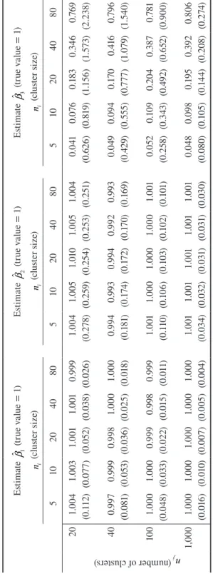
The results of the simulation for the linear two-level multilevel model are presented in Table 1 and in Figures 1, 2, and 3.
The results show that there are very low levels of bias in the estimates of βˆ1,
the regression weight associated with the level 1 variable
x
ij (Table 1). Even underextreme conditions (ni = 5 and nj = 20), the estimated regression weights were
very close to the true value. This is also apparent from Figure 1, which displays the mean percentage relative bias in βˆ1. In all conditions, the percentage relative bias
is below +/- 1%. Bias decreases on average if the cluster size or if the number of clusters increases, as can be seen from Figure 1. As regards the estimate βˆ2 – the
regression weight associated with the level 2 variable cj– the results similarly show only insubstantial bias in the estimates (Table 1). Again, the percentage relative bias does not exceed +/- 1% in any condition (Figure 2). Bias decreases further when the number of level 2 units increases (Figure 2). Accordingly, for both βˆ1 and
2
ˆ
β bias caused by level 1 sparseness appears negligible.
However, the results show a strikingly different picture when it comes to the estimate of βˆ3, the regression weight associated with the cluster mean
'
j
x . Again, the true value for the parameter was set to equal 1. If the cluster size is very small (ni = 5), the estimated regression weights show an extreme downward bias being
close to zero (Table 1). Bias decreases when the size of the clusters increases – from an average percentage relative bias of -95.25% in the condition of extreme level 1 sparseness (ni = 5) to -21.20% if the clusters comprise 80 level 1 observations
(ni = 80) (Figure 3). Even with moderate cluster sizes, i.e. ni = 40, the average
per-centage relative bias is still -59.94. Importantly, bias does not decrease if the num-ber of clusters increases. The numnum-ber of level 2 units (nj = 20, 40, 100, 1000) is not
statistically significantly related to the size of the bias (ni = 5: F (3, 3996) = 0.15,
p<0.932;
n
i = 10: F (3, 3996) = 0.65, p<0.582; ni = 20: F (3, 3996) = 0.39, p<0.759; iTa bl e 1 Es tim at ed r eg re ss io n w eig ht s ( me an s a nd s ta nd ar d d ev iat io ns ) Es tima te 1
ˆ (tβ
ru
e v
al
ue = 1
)
i
n (c
lus ter si ze ) Es tima te 2
ˆ (tβ
ru
e v
al
ue = 1
)
i
n (c
lus ter si ze ) Es tima te 3
ˆ (tβ
ru
e v
al
ue = 1
)
i
n (c
-2 -1.5 -1 -.5 0 .5 1
R
el
at
iv
e bi
as
(%
)
0 20 40 60 80
Size of clusters / groups 20 40 100 1,000 Number level 2 units (clusters)
Figure 1 Percentage relative bias in βˆ1
-2 -1.5 -1 -.5 0 .5 1
R
el
at
iv
e bi
as
(%
)
0 20 40 60 80
Size of clusters / groups 20 40 100 1,000 Number level 2 units (clusters)
Figure 2 Percentage relative bias in βˆ2
-100 -80 -60 -40 -20 0
R
el
at
iv
e bi
as
(%
)
0 20 40 60 80
Size of clusters / group size 20 40 100 1,000 Number level 2 units (clusters)
4 Conclusions
The results of this study show that level 1 sparseness (i.e. small cluster size) in multilevel models can cause large bias in estimated regression weights of level 2 variables that are aggregated from level 1 variables.
To assess the effect of level 1 sparseness, this study simulated multilevel data varying the number and the size of clusters and analyzed the data to evaluate the impact of level 1 sparseness on the estimated regression weights. The number and size of clusters had relatively little impact on the estimated effect of regression weights of normal level 1 and level 2 variables. In this respect, this study links up with previous research (Bell et al., 2008; Clarke, 2008; Clarke & Wheaton, 2007; Maas & Hox, 1999, 2005).
However, if multilevel models include level 2 variables that are a function of the level 1 variables, e.g. the average income or the proportion of unemployed people in a neighborhood, the study found severe downward bias in estimated regression weights. In situation of extreme level 1 sparseness, that is if the clusters comprise only 5 or 10 observations, the average percentage relative bias was more than 93%. Importantly, bias does not decrease if the number of level 2 units increases. Bias reduces if the number of observations within each cluster increases. However, even with moderate cluster sizes (20 or 40 observations per cluster), bias is still substan-tial.
What is the reason for such bias? Reliability of aggregated variables depend on cluster size (Snijders & Bosker, 2004, pp. 25-26). If very few level 1 units are used to generate the level 2 characteristic, we are dealing with measurement error: The (aggregated) level 2 characteristic is a noisy estimate of the true level 2 characteris-tic. It is a well-known fact that error-in-variables causes attenuation (i.e. downward) bias in estimated regression weights in linear models (Wooldridge, 2010, p. 81). The problem we are therefore facing is a measurement error or error-in-variables problem, respectively.
We have to assume that this is a prevalent problem. Most multilevel data comprise samples of level 1 units drawn out of a population of level 2 units, e.g. respondents living in larger neighborhoods, students attending different schools, or employees working in different establishments. In all these data, estimated effects of aggregated level 2 variables will be biased downward.
Obviously, the problem only applies if the clusters are samples. If the multilevel data comprises the full clusters, i.e. if all observations within a cluster are included, such as all students nested in a class, the problem will not apply – even if the clus-ters are small.
aggregated level 2 characteristics. For instance, administrative data may be used to complement survey data with the level 2 variables of interest. A third remedy lies in methods that adjust for measurement error. Measurement error can, for instance, be accommodated by using a latent variable approach (Bollen, 1989; Reinecke & Pöge, 2010; Skrondal & Rabe-Hesketh, 2003). This would require using multiple level 1 indicators to model the (latent) level 2 characteristic. For instance, neighbor-hood characteristics could be assessed by relying on several measures, e.g. (mean) income, (mean) education, (proportion of) unemployment, etc. While these three potential remedies appear promising, one may still encounter situations in which none is applicable and should therefore treat aggregated variables in multilevel models with caution.
References
Allison, P. D. (2009). Fixed effects regression models. Los Angeles: SAGE.
Bell, B. A., Ferron, J. M., & Kromrey, J. D. (2008). Cluster size in multilevel models: the impact of sparse data structures on point and interval estimates in two-level models.
JSM Proceedings, Section on Survey Research Methods, 1122-1129. Bollen, K. A. (1989). Structural equations with latent variables. New York: Wiley.
Clarke, P. (2008). When can group level clustering be ignored? Multilevel models versus single-level models with sparse data. Journal of Epidemiology and Community Health, 62(8), 752-758.
Clarke, P., & Wheaton, B. (2007). Addressing data sparseness in contextual population re-search using cluster analysis to create synthetic neighborhoods. Sociological Methods & Research, 35(3), 311-351.
De Leeuw, J., Meijer, E., & Goldstein, H. (2008). Handbook of multilevel analysis: Springer. Fauth, R. C., Roth, J. L., & Brooks-Gunn, J. (2007). Does the neighborhood context alter
the link between youth’s after-school time activities and developmental outcomes? A multilevel analysis. Developmental Psychology, 43(3), 760.
Gross, C., & Kriwy, P. (2013). Einfluss regionaler sozialer Ungleichheits- und Arbeitsmarkt-merkmale auf die Gesundheit.
Hox, J. (1998). Multilevel modeling: When and why Classification, data analysis, and data highways (pp. 147-154): Springer.
Kreft, I. G. (1996). Are multilevel techniques necessary? An overview, including simulation studies: California State University Press, Los Angeles.
Langer, W. (2010). Mehrebenenanalyse mit Querschnittsdaten. In C. Wolf & H. Best (Eds.),
Handbuch der sozialwissenschaftlichen Datenanalyse (pp. 741-774). Wiesbaden: Springer.
Maas, C. J., & Hox, J. J. (1999). Sample sizes for multilevel modeling. American Journal of Public Health, 89, 1181-1186.
Maas, C. J., & Hox, J. J. (2005). Sufficient sample sizes for multilevel modeling. Methodo-logy, 1(3), 86-92.
Rabe-Hesketh, S., & Skrondal, A. (2012). Multilevel and longitudinal modeling using Stata
(3rd ed.). College Station, Tex.: Stata Press Publication.
Raudenbush, S. W., & Bryk, A. S. (2002). Hierarchical Linear Models. Applications and Data Analysis Methods. Thousand Oaks: Sage.
Reinecke, J., & Pöge, A. (2010). Strukturgleichungsmodelle. In H. Best & C. Wolf (Eds.),
Handbuch der sozialwissenschaftlichen Datenanalyse (pp. 775-804). Wiesbaden: VS. Schunck, R. (2013). Within- and Between-Estimates in Random Effects Models.
Advanta-ges and Drawbacks of Correlated Random Effects and Hybrid Models. Stata Journal, 13(1), 65-76.
Schunck, R., & Windzio, M. (2009). Ökonomische Selbstständigkeit von Migranten in Deutschland: Effekte der sozialen Einbettung in Nachbarschaft und Haushalt. Zeit-schrift für Soziologie, 38(2), 111-128.
Skrondal, A., & Rabe-Hesketh, S. (2003). Some applications of generalized linear latent and mixed models in epidemiology: repeated measures, measurement error and multilevel modeling. Norsk epidemiologi, 13(2).
Snijders, T. A., & Bosker, R. J. (2004). Multilevel Analysis. An Introduction to Basic and Advanced Multilevel Modeling. London: Sage.
Snijders, T. A., & Bosker, R. J. (2012). Multilevel analysis. An introduction to basic and advanced multilevel modeling (2nd ed.). Los Angeles: Sage.
StataCorp. (2013). Stata: Release 13. Statistical Software. College Station, TX: StataCorp LP.
Windzio, M. (2004). Kann der regionale Kontext zur „Arbeitslosenfalle “werden? KZfSS Kölner Zeitschrift für Soziologie und Sozialpsychologie, 56(2), 257-278.
Windzio, M., & Teltemann, J. (2013). Empirische Methoden zur Analyse kontextueller Fak-toren in der Bildungsforschung Bildungskontexte (pp. 31-60): Springer.
Appendix
// Stata code
clear all version 13.1
global data "..." // define file path here
// #1
// define program
capture program drop l2linear program define l2linear clear
drop _ all args i j set obs 'j' gen j = _ n
gen c _ j = rnormal(0,1) gen u _ j = rnormal(0,1) expand 100
bysort j: gen i = _ n gen x _ ij = rnormal(0,1)
bysort j: egen x _ j = mean(x _ ij) gen e _ ij = rnormal(0,1)
gen y _ ij = 1 + 1*x _ ij + 1*c _ j + 1*x _ j + u _ j + e _ ij bysort j: sample 'i', count
bysort j: egen x _ j _ noise = mean(x _ ij) xtreg y _ ij x _ ij x _ j _ noise c _ j, i(j) re end
// #2 // simulate
foreach j of numlist 20 40 100 1000 { foreach i of numlist 5 10 20 40 80 {
simulate _ b, seed(12345) reps(1000): l2linear 'i' 'j' gen n _ j = 'j'
gen n _ i = 'i' sum
if ('j'==20 & 'i'==5) save "${data}\sim _ linear.dta", replace else {
append using "${data}\sim _ linear.dta" save "${data}\sim _ linear.dta", replace }