www.clim-past.net/12/151/2016/ doi:10.5194/cp-12-151-2016
© Author(s) 2016. CC Attribution 3.0 License.
The effect of a dynamic soil scheme on the climate of the
mid-Holocene and the Last Glacial Maximum
M. Stärz1,2,3, G. Lohmann1,4, and G. Knorr1
1Alfred Wegener Institute Helmholtz Centre for Polar and Marine Research, Bremerhaven, Germany
2Senckenberg Research Institute and Natural History Museum, Frankfurt am Main, Germany
3Biodiversity and Climate Research Centre (LOEWE BiK-F), Frankfurt am Main, Germany
4University of Bremen, Bremen, Germany
Correspondence to: M. Stärz ([email protected])
Received: 7 May 2013 – Published in Clim. Past Discuss.: 24 May 2013
Revised: 13 December 2015 – Accepted: 17 December 2015 – Published: 29 January 2016
Abstract.In order to account for coupled climate–soil pro-cesses, we have developed a soil scheme which is asyn-chronously coupled to a comprehensive climate model with dynamic vegetation. This scheme considers vegetation as the primary control of changes in physical soil characteristics. We test the scheme for a warmer (mid-Holocene) and colder (Last Glacial Maximum) climate relative to the preindustrial climate. We find that the computed changes in physical soil characteristics lead to significant amplification of global cli-mate anomalies, representing a positive feedback. The in-clusion of the soil feedback yields an extra surface warm-ing of 0.24◦C for the mid-Holocene and an additional global cooling of 1.07◦C for the Last Glacial Maximum. Transi-tion zones such as desert–savannah and taiga–tundra exhibit a pronounced response in the model version with dynamic soil properties. Energy balance model analyses reveal that our soil scheme amplifies the temperature anomalies in the mid-to-high northern latitudes via changes in the planetary albedo and the effective longwave emissivity. As a result of the modified soil treatment and the positive feedback to cli-mate, part of the underestimated mid-Holocene temperature response to orbital forcing can be reconciled in the model.
1 Introduction
The signature of climate variability on orbital timescales (i.e. mid-Holocene, 6 kyr ago, and Last Glacial Maximum, 21 kyr ago) as derived from proxy archives serves as a test bed for a critical evaluation of general circulation models
type had changed. The integrated vegetation–soil feedback reinforced glacial cooling to some extent (Jiang, 2008). Fur-ther progress is shown in Vamborg et al. (2011), in which the authors implemented a dynamic background albedo scheme within a comprehensive fully coupled GCM with vegetation dynamics (earth system model, ESM). In this model, the model additionally accounts for land surface albedo changes based on the calculation of carbon fluxes between terrestrial carbon pools (vegetation, litter and phytomass, and soil).
So far, various studies have focused on the climate effect of physical soil parameter changes. However, the combined impact and feedback of soil albedo, texture, and total water-holding field capacity within the fully coupled atmosphere– vegetation–ocean system remains to be addressed. The cur-rent inability of comprehensive state-of-the-art ESMs to compute the dynamics of physical soil characteristics reveals a potential failure to represent paleoclimate dynamics and quantifying paleoclimate sensitivity.
Here, we investigate the impact of dynamic soils on the cli-mate of the mid-Holocene and the Last Glacial Maximum by means of the comprehensive ESM with vegetation dynamics, COSMOS (Community of Earth System Models; Jungclaus et al., 2006; Raddatz et al., 2007). We develop a simple soil scheme which incorporates the computation of soil albedo, soil texture, and total water-holding field capacity and cou-ple this asynchronously to the ESM. The coucou-pled version of COSMOS allows us to examine the potential soil feedback in the atmosphere–vegetation–ocean system.
The model approach utilizes boundary conditions of the preindustrial period, the mid-Holocene, and the Last Glacial Maximum (LGM). The simulations of the extended model set-up are further compared to the respective standard time-slice studies (Wei and Lohmann, 2012; Zhang et al., 2013) to show that dynamic soils drive significant positive feedbacks in the coupled climate system for past climate states.
2 Methods
We use the ESM configuration presented by Jungclaus et al. (2006) and describe the design of the soil scheme and the asynchronous coupling procedure. The experimental design includes a short description of the applied model boundary conditions that are representative of the mid-Holocene and LGM (Wei and Lohmann, 2012; Zhang et al., 2013). Further-more, a forcing factor separation method (Stein and Alpert, 1993; Zhang et al., 2015) has been applied to isolate the po-tential soil feedback in the climate system.
2.1 Model description
In the current ESM set-up, three model components (at-mosphere, sea-ice–ocean, land surface) are coupled to each other within the COSMOS model suite. The atmospheric component of COSMOS is ECHAM5 (Roeckner et al., 2003), with a spectral resolution of T31L19 (3.75×3.75◦
horizontal grid-space resolution and 19 vertical layers), which enables a direct comparison with previous studies of the mid-Holocene and LGM (Wei and Lohmann, 2012; Zhang et al., 2013). The ocean model MPIOM uses an or-thogonal curvilinear grid (3◦×1.5◦lateral resolution) with a higher resolution at the grid poles (Greenland, Antarc-tica) and 40 unevenly spaced vertical layers (Marsland et al., 2003). The transfer of fluxes and momentum between atmo-sphere and ocean is handled by the coupler OASIS3 with-out any flux corrections (Jungclaus et al., 2006). The mod-ular land surface scheme JSBACH (Raddatz et al., 2007) with vegetation dynamics (Brovkin et al., 2009) is embed-ded in the ECHAM5 atmosphere model. JSBACH is based on the semiempirical terrestrial ecosystem model BETHY, which incorporates an energy and water balance, photosyn-thesis, phenology, and a carbon balance compartment (Knorr, 2000). JSBACH employs a subgrid-scale tiling approach in which the actual cover fraction of each plant functional type (PFT) is associated with a tile within each grid cell. In our study, JSBACH uses the standard model configuration of eight PFTs. The land surface energy balance considers soil albedo, leaf area index of the actual PFT, the albedo of stems, snow fraction on the ground and on the canopy, and the mask-ing effect of snow under the canopy. Further background in-formation on COSMOS and its components can be found in Jungclaus et al. (2006). So far, COSMOS has been applied to various palaeo set-ups such as the Holocene (Wei et al., 2012; Wei and Lohmann, 2012; Varma et al., 2012; Lohmann et al., 2013), Last Glacial Maximum and Marine Isotope Stage 3 (Gong et al., 2013; Zhang et al., 2013, 2014), last interglacial (Lunt et al., 2013), Pliocene (Stepanek and Lohmann, 2012), and Miocene (Knorr et al., 2011; Knorr and Lohmann, 2014).
2.2 Design of the soil scheme
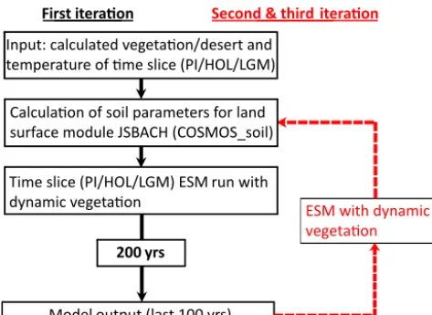
The design of the soil scheme is based on the concept that an organism actively regulates and transforms its abiotic envi-ronment (Lovelock, 1979). We therefore specify soil types that correspond to PFTs. Applying this concept, the soil scheme diagnoses soil types by the composition of computed PFTs for each grid cell. The computed PFTs are derived from the land surface model JSBACH (Fig. 1; see Sect. 2.4). This procedure does not explicitly capture all pedogenic factors (e.g. parent rock; Targulian and Krasilnikov, 2007); however, some may be indirectly considered by vegetation demands (e.g. plant water accessibility, viable temperature limits). The aim of the soil type classification is to provide constraints of physical characteristics (total water-holding field capacity, albedo, and texture) for the land surface scheme of COSMOS and therefore does not refer to the pedologic nomenclature.
Model output (last 100 yrs)
ESM with dynamic vegetation FFFF
First iteration Second & third iteration
200 yrs
Input: calculated vegetation/desert and temperature of time slice (PI/HOL/LGM)
Time slice (PI/HOL/LGM) ESM run with dynamic vegetation
Calculation of soil parameters for land surface module JSBACH (COSMOS_soil)
Figure 1.Flowchart of the asynchronous coupling procedure
be-tween the earth system model (ESM) and the soil scheme (COS-MOS_soil). (PI: preindustrial period; HOL: mid-Holocene.)
including an asynchronous coupling time step of 200 years between COSMOS and the soil scheme. Thus, for a model integration period of 600 years, the soil scheme iterates three times in total. The asynchronous coupling is defined by us-ing the previous 100-model-year mean of COSMOS as in-put for the soil scheme (Fig. 1). Within this study, the cou-pled version of the ESM with the soil scheme is called COS-MOS_soil. At the end of the model simulation, the final 100 years of model integration, including the physical soil char-acteristics of the third iteration are used for analysis.
2.3 Deriving physical soil characteristics
The physical soil characteristics of JSBACH comprise snow-free soil albedo (α) in the visible (αvis, 0.3–0.7 µm) and near-infrared (αnir, 0.7–3 µm) light spectrum, total water-holding field capacity of soil (hcws), and soil data flags (soil texture) from the United Nations Food and Agriculture Organiza-tion (FAO) soil classificaOrganiza-tion (Hagemann et al., 1999; Hage-mann, 2002; Rechid et al., 2009). The original data set of the snow-free soil albedo is derived from modified satellite measurements of the Moderate Resolution Imaging Spectro-radiometer (MODIS; Rechid et al., 2009). The FAO soil data flags (refer to Gildea and Moore in Henderson-Sellers et al., 1986) represent a general grain size classification ranging from sand to clay. The assessment of the total water-holding field capacity of soils (hcws) reveals considerable uncertain-ties and is estimated by a data set of the parameterhpwp (per-manent wilting point) andhava (maximum amount of water that plants may extract from the soil before they start to wilt), which is based on optimised rooting depths (Hagemann et al., 1999).
To derive physical soil characteristics that agree with veg-etation changes, we use calculated PFTs from the final 100-year mean of a preindustrial model output (Wei et al., 2012;
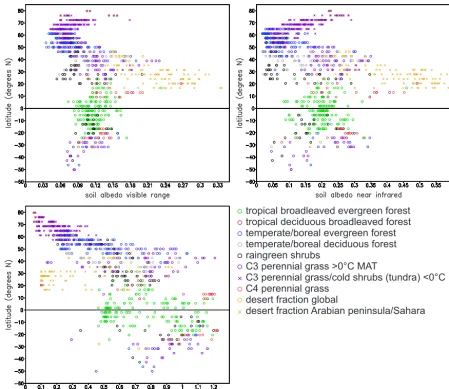
Fig. 2). Physical soil characteristics are specified for all dom-inant PFTs (defined by a cover fraction > 50 % of the grid cell) by global mean calculation (Table 1). Additionally, we define a soil type that represents global desert areas (de-fined by the cover fraction that lacks vegetation cover for > 50 model years) and a subgroup specifying the Arabian Peninsula–Sahara desert region (defined by < 50 % vegeta-tion cover within a zonal belt of 13–35.26◦N). The desert subgroup is mandatory when considering extremes ofhcws and soil albedo values of bare soils (Fig. 2, yellow crosses). Further, we subdivide C3 grass into “warm-tolerance” (de-fined by the mean annual temperature, MAT, > 0◦C) and “cold-tolerance grass” (MAT < 0◦C). In total, the adjusted classification consists of 10 soil types (Fig. 2, Table 1). The FAO soil data flags constitute a coarse-soil texture classifica-tion, ranging from 1 (sand) to 5 (clay), and are rather insen-sitive to the specified soil types (Table 1). Though calculated by the soil scheme, we do not further consider this variable in our study.
2.4 Soil scheme
The soil scheme computes grid-cell-specific soil character-istics soln (n refers to hcws, fao, αs,vis,αs,nir) according to the soil classification described in Sect. 2.3. The soil char-acteristic soln is calculated by a soil index. The soil index
includes the cover fraction of the soil types (fi), which are
generally derived by PFT-specific cover fractions (Table 1). The soil index weights the soil characteristic of a specific soil type (fisoli) by the cumulative cover fraction of all soil types
P10
i=1fiper grid cell:
soln=
P10
i=1(fisoli)
P10
i=1fi
. (1)
IfP10
i=1fi does not occupy the full grid cell space, the
residual is interpreted as desert (see Sect. 2.3, Table 1). The weighted soil characteristics are summed to a grid cell av-erage of soil characteristics and thereafter transferred to the atmospheric component of COSMOS.
2.5 Experimental design
We investigate the soil feedback for three different time slices: the preindustrial period (PI_ctl; Wei et al., 2012), the mid-Holocene (HOL_ctl, 6 kyr before present; Wei and Lohmann, 2012), and the LGM (LGM_ctl;∼21 kyr before present, Zhang et al., 2013). All time-slice model simulations are performed by the standard COSMOS configuration. The model simulations utilise background conditions and forcing parameters described by the PMIP3 protocol (Paleoclimate Modelling Intercomparison Project; Braconnot et al., 2012) and are run until they reach equilibrium.
tropical broadleaved evergreen forest tropical deciduous broadleaved forest temperate/boreal evergreen forest temperate/boreal deciduous forest raingreen shrubs
C3 perennial grass >0°C MAT
C3 perennial grass/cold shrubs (tundra) <0°C MAT C4 perennial grass
desert fraction global
desert fraction Arabian peninsula/Sahara
Figure 2.Physical soil properties (abscissa) used in the dynamical vegetation module JSBACH associated with plant functional types along latitudes. Albedo values are derived from modified satellite measurements of the Moderate Resolution Imaging Spectroradiometer (MODIS; Rechid et al., 2009), and total water-holding field capacity of soils are taken from Hagemann et al. (1999).
gases as compared to the preindustrial period (Wei et al., 2012). Adjustments of LGM boundary conditions include or-bital parameter settings, greenhouse gases, sea-level and ice sheet changes, and an initial salinity change in the glacial ocean by+1 ‰ (Zhang et al., 2013). The length of the sim-ulations PI_ctl, HOL_ctl, and LGM_ctl amounts to at least 3000 years for each model run (Wei et al., 2012; Zhang et al., 2013). The model simulations, including dynamic soils, refer to the respective time-slice model simulation (PI_ctl, HOL_ctl, LGM_ctl) and continue the integration for another 600 years in total. All model output shows mean climate con-ditions for the final 100 years of the simulations.
2.6 Analysis of the soil feedback to the climate system The respective soil feedback to the climate of the mid-Holocene and the LGM is analysed by using a factor
sepa-ration method for identifying synergies in numerical mod-els (Stein and Alpert, 1993; Lunt et al., 2012; Zhang et al., 2015). The method calculates the effect between ap-plied changes to a reference state with respect to an unper-turbed reference state (f0,0), e.g. the calculated single effect of changing two forcing factorsf1,0andf0,1separately, as well as the combination of both factorsf1,1. Thereafter, the synergetic effectfˆ1,1between both factors can be calculated (Stein and Alpert, 1993). To isolate the synergetic effectfˆ1,1 between the two factors, the anomaly term of their linear combinations is calculated:
ˆ
f1,1=f1,1−f1,0−f0,1+f0,0. (2)
Devi-T ab le 1. Specified soil types and associated ph ysical soil characteristics. (VIS: visible spectrum; NIR: nea r-infrared spectrum.) Soil types based on calculated PFTs Ph ysical soil characteristics (sol n ) hcws , total w ater -holding soil te xture, F A O soil αvis , soil albedo VIS αnir , soil albedo NIR field capacity of soil (metres) data flags (0.3–0.7 µm) (0.7–3 µm) T ropical broadlea v ed ev er green forest 0.77 loam and clay 0.12 0.20 T ropical deciduous broadlea v ed forest 0.73 loam 0.18 0.34 T emper . or boreal ev er green forest 0.50 loam 0.08 0.10 T emper . or boreal deciduous forest 0.58 loam 0.09 0.11 Raingreen shrubs 0.68 loam 0.12 0.17 C3 perennial grass C3 perennial grass > 0 ◦C MA T 0.77 loam 0.12 0.21 C3 perennial grass or cold shrubs (tundra) < 0 ◦C MA T 0.23 loam 0.08 0.13 C4 perennial grass 1.07 loam 0.14 0.26 Desert fraction global desert fraction 0–100 % 0.17 loam 0.20 0.37 Sahara–Arabian Peninsula desert fraction > 50 % (13–35.26 ◦N) 0.11 loam 0.25 0.49
ations from 0 indicate nonlinearities (climate feedbacks) in the system.
By means of the factor separation method, the model simulations are factorised representing the background cli-mate (fclimate,0) and dynamic soils (f0,soil). Thereafter, we disentangle the joint effect of climate and dynamic soils
(fclimate,soil), which we call soil feedback. The soil feedback
is indicated byfˆclimate,soil:
ˆ
fclimate,soil=fclimate,soil−fclimate,0−f0,soil+f0,0. (3)
The factorsf0,0 andf0,soil refer to the preindustrial model run without (PI_ctl) and with dynamic soils (PI_sol), re-spectively. The defined background climate of the model run
fclimate,0represents several changes in the boundary
condi-tions with respect to the preindustrial period that are applied for each time slice (mid-Holocene, LGM; see Sect. 2.5), and the “dynamic soils” factorf0,soilrefers to model runs, which have been performed including the interactive soil scheme (COSMOS_soil). The combination of both factors is given
byfclimate,soil.
The forcing of the mid-Holocene model run is mainly driven by insolation anomalies as compared to the prein-dustrial period; therefore, the soil feedback is largely at-tributed to changes in orbital forcing. However, the multitude of changes in the LGM boundary conditions that is represen-tative of the LGM background climate (see Sect. 2.5) does not allow the identification of a monocausal relationship. The calculated soil feedback of the respective model studies is presented in Sects. 3.1 and 3.2.
3 Results
This section gives a brief presentation on the climate anoma-lies, which are introduced by coupling of the soil scheme and the ESM for the preindustrial period. In the next step, the simulated mid-Holocene and LGM climate that are de-rived from the extended model set-up including dynamic soils (COSMOS_soil) are described, and, thereafter the soil feedback to the respective climate state is shown.
3.1 Preindustrial simulation (PI_sol – PI_ctl)
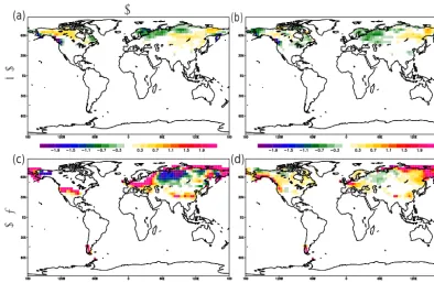
The preindustrial mean surface air temperature (SAT), precipitation, and evaporation anomalies between COS-MOS_soil and COSMOS (PI_sol – PI_ctl) show the effect of coupling the soil scheme to the ESM (Fig. 3). In general, the global mean SAT increases by 0.27◦C. High northern lat-itude SATs locally increase by about 1◦C at the Canadian Arctic Archipelago, and Baffin Bay is affected by reduced sea-ice cover as a consequence of changes in the soil charac-teristics. Regional warming in remote areas like the Southern Ocean is sensitive to sea-ice changes as a function of anoma-lous wind fields and ocean current shifts.
(a)
(b)
(c)
(d)
(e)
(f)
PI_sol - PI_ctl
Figure 3.Differences in 100-year annual mean of the preindustrial climate state with dynamic soils and fixed soil characteristics (PI_sol – PI_ctl) included for (a) surface air temperature in degrees Celsius, (b) total precipitation in millimetres per day, (c) evaporation in kilograms per square metre per day, (d) forest fraction, (e) grass fraction, and (f) desert fraction. Hatched areas identify non-significant values, calculated by means of a Studentttest with 0.05 levels of significance.
latitudes (60–90◦N). The Arabian Peninsula and Sahara re-gion exhibit relatively strong temperature anomalies caused by the threshold parameterization (see Sect. 2.3) and the ab-sence of vegetation covering the ground. Precipitation and evaporation anomalies in the low latitudes are typically af-fected by anomalous changes in the inner tropical conver-gence zone (Fig. 3b, c). On a global scale, the total water-holding field capacity of soils increases (+0.06 m) with re-spect to PI_ctl (0.63 m), but the global soil water budget is
slightly reduced (−0.008 m). In PI_sol the simulated for-est cover slightly increases in high latitudes and decreases in subtropical regions where it is replaced by grass cover (Fig. 3d, e). In the subtropical areas (30◦S–30◦N), grass cover increases at the expense of forest cover, likely due to a reduction in the total water-holding field capacity.
(a)
(c)
(b)
(d)
ΔT
fˆLGM
HOL
Figure 4.Surface air temperature (◦C) anomalies of a 100-year annual mean climate state with respect to the preindustrial period for (a) mid-Holocene (HOL_sol – PI_sol), (b) mid-Holocene soil feedback (fˆ
HOL,soil), (c) Last Glacial Maximum (LGM_sol – PI_sol), (d) Last
Glacial Maximum soil feedback (fˆ
LGM,soil). A nonlinear scaling is used for the colour bar displayed in panel (c). Hatched areas identify
non-significant values, calculated by means of a Studentttest with 0.05 levels of significance.
steady-state conditions. Therefore, soil characteristics in a fi-nal state may not reflect the same status of present soil char-acteristics. For a more detailed discussion, the reader is re-ferred to the beginning of Sect. 4.
3.2 Mid-Holocene climate (HOL_sol – PI_sol)
The application of Holocene boundary conditions to COS-MOS_soil (HOL_sol) leads to a global surface air tem-perature (SAT) warming of 0.34◦C with respect to PI_sol. The anomalous SAT warming of the standard Holocene model simulation (HOL_ctl – PI_ctl: +0.1◦C) undergoes a substantial temperature rise by including the soil feed-back (fˆ
HOL,soil= +0.24◦C). High northern latitudes exhibit
largest amplitudes, i.e. the Barents Sea is affected by sea-ice retreats (Fig. 4). Hatched areas shown in Fig. 4 and the sub-sequent Figs. 5 and 6 mark anomalies in regions with no sig-nificant climate change (significance level: 0.05). A general feature of the mid-Holocene climate pattern is given by nega-tive temperature anomalies, accompanied by significant pre-cipitation (Fig. 5) and evaporation anomalies (Fig. 6), which arise especially in regions that are sensitive to the African and Asian monsoon. In principle, the mid-Holocene land
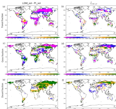
surface is basically characterised by higher forest (+2.3 %) and grass abundance (+1.2 %) at the expense of desert frac-tion (−3.9 %). More specifically, the forest cover expands in northern Canada, northern Siberia and at the Sahara– Sahel transition; this expansion is accompanied by anoma-lous warming (Fig. 4) and increasing precipitation (Fig. 5), respectively, or a combination of these two factors. Simul-taneously, decreased forest fraction is simulated in regions exhibiting negative precipitation anomalies with respect to PI_sol, as can be exemplarily seen in the South America trop-ical rainforests (Fig. 7).
(a)
(c)
(b)
(d)
LGM
HOL
ΔT
fˆFigure 5.As Fig. 4 but for total precipitation (mm day−1).
which in turn contributes to elevated land surface runoff and drainage (+3.35 kg m−2yr−1).
Globally, the land surface albedo decreases by 0.011, with maximum temperature anomalies at the transition zone of the Sahara–Sahel region. This is accompanied by changes in soil characteristics and a northward migration of vegetation to-wards the Sahara desert (Fig. 4). The high northern latitudes, in particular, undergo a “darkening” of the land surface due to the integrated effect of lowered soil albedo (Fig. 8), albedo effects caused by the expansion of forest cover (Fig. 7), and regional snow depth changes (given in millimetres of wa-ter equivalent) in the continental realm of the Barents Sea (Fig. 10). The replacement of C3 grass by forest in these lo-cations increases vegetation canopy and governs associated changes in soil characteristics: a higher abundance of bo-real evergreen forests in the high northern latitudes leads to a decreased soil albedo and to an increase in the total water-holding field capacity relative to soils that are associated with C3 grasses.
3.3 LGM climate (LGM_sol – PI_sol)
The LGM climate, as calculated in COSMOS_soil (LGM_sol), reveals an overall global SAT cooling of 7.03◦C. The impact of the implemented soil scheme
(fˆLGM,soil) yields an additional cooling of 1.07◦C with
(a)
(c)
(b)
(d)
ΔT
fˆLGM
HOL
Figure 6.As Fig. 4 but for evaporation (kilograms per square metre per day).
in the high northern latitudes (Fig. 10). Interestingly, forest cover increases slightly along ∼30◦S most likely as a response to greater precipitation there. Tropical forest cover is drastically reduced by 59 % compared to PI_sol. In most areas grasses replace forests, and deserts (e.g. in the Arabian Peninsula, Sahara–Sahel borderline, and northern Siberia) expand at the expense of grasses.
The computed change in physical soil characteristics shows a general decrease inhcws(−8.3 cm; Fig. 8b) as a re-sponse to climate and vegetation change. However, this effect is mainly compensated for (global meanhcws, including sub-aerial shelf regions:−0.4 cm) by considering additional soil processes in subaerial regions, as an effect of the sea level drop (Fig. 8b). The strongest decline in total water-holding field capacities of soils is localised at the southern border-line of the Eurasian and Laurentide ice sheets and the Sa-hara desert. This responds to a decrease in surface tempera-tures and precipitation, which is in line with a reduction in the forest fraction and a parallel expansion of the desert area (Fig. 11a, e).
Comparing Figs. 8b and 9b, the total water-holding field capacity of soils constitutes a direct soil wetness control. Thereby, elevated soil wetness along the∼30◦S latitudinal band (Fig. 9b) is not directly linked tohcwsbut rather reflects a change in atmospheric circulation that is associated with
in-creased precipitation, evaporation, and forest cover (Figs. 5c, 6c, 11a).
(a)
(c)
(e)
(b)
(d)
(f)
HOL_sol - PI_sol fˆHOL,soil
Desert fraction
Grass fraction
Forest fraction
Figure 7.Vegetation differences in 100-year mean of the mid-Holocene and preindustrial climate state with dynamic soils (HOL_sol –
PI_sol) and enclosed soil feedback (fˆHOL,soil) included for (a) forest fraction and (b) soil impact on forest fraction, (c) grass fraction and (d)
soil impact on grass fraction, (e) desert fraction and (f) soil impact on desert fraction.
3.4 Energy balance model
To separate the effect of radiative components of the iso-lated soil feedback on the respective climate, we additionally present results of a zero-dimensional energy balance model. The radiative balance of the soil feedback is quantified by applying a zero-dimensional energy balance model (0-dim EBM) for a grey atmosphere (Sellers, 1969):
(1−α)S/4=εσ T4. (4)
The 0-dim EBM comprises the total irradiance (S=1367 Wm−2), the Stefan–Boltzmann constant (σ =5.67×10⁻⁸Wm−2K−4), the planetary albedo α, and the effective longwave emissivity ε. The planetary albedo is calculated by the ratio of incoming and outgoing shortwave radiation at the top of the atmosphere, and the effective longwave emissivity is given by the fraction of outgoing longwave radiation at the top of the atmosphere and the surface – all radiative fluxes are provided by the
globally and regionally averaged model output. Thereafter, the radiative equilibrium temperature T is derived by the 0-dim EBM.
For the preindustrial period (PI_ctl) the 0-dim EBM con-stitutes a planetary albedo of 0.32 and an effective longwave emissivity of 0.584, which equals a radiative equilibrium temperature of 289.4 K, in line with previous EBM consid-erations (Heinemann et al., 2009). To compare the radiative contributions in the prevailing model studies,αandεare ex-pressed in terms of temperature anomalies with respect to the preindustrial period (Fig. 12). Motivated by the 0-dim EBM, we apply radiation diagnostics at the surface on a regional scale comprising the tropics (30◦S–30◦N) and mid-to-high northern latitudes (30–90◦N).
For the mid-Holocene and LGM (without dynamic soils), the 0-dim EBM calculates a similar warming (+0.1◦C) and cooling (−5.4◦C), respectively, as for the global SAT changes in the model simulations (HOL_ctl – PI_ctl:
(a)
(b)
/and surface albedo
6oil albedo near-infrared
6oil albedo visible range
LGM
HOL
Field capacity of soil (m)
Figure 8. Changes in water-holding field capacities (metres) in soils and zonally averaged land surface albedo and soil albedo for (a) mid-Holocene (HOL_sol – PI_sol) and (b) Last Glacial Maximum (LGM_sol – PI_sol).
(a)
(c)
(b)
(d)
LGM HOL
(a)
(b)
(c)
(d)
LGM
HOL
ΔT
fˆFigure 10.As Fig. 4 but for snow depth (water equivalent in millimetres).
albedo and effective longwave emissivity contribute to an amplification of the original temperature anomaly, taking dy-namic soils into account. The anomaly of COSMOS_soil and COSMOS with respect to the preindustrial period (PI_sol – PI_ctl: +0.1◦C) shows the error of procedure by includ-ing the soil scheme in the model set-up (see Sect. 3.1). This anomaly accounts for the offset between model runs with and without dynamic soils and should be considered in the com-parison of the two model versions. As a reference, the re-gional and global deviations regarding the error of procedure (PIsol) are displayed as well (Fig. 12). Nevertheless, we state that anomalies between model studies with (COSMOS_soil) and without the interactive dynamic soil component (COS-MOS) consistently reveal stronger soil effects as compared to the error of procedure (PIsol).
Interestingly, based on the 0-dim EBM analysis the Holocene temperature rise without dynamic soils (+0.1◦C) is solely attributed to a reduction in the effective longwave emissivity, corroborated by an increase in the water vapour content in the atmosphere (+0.28 kg m−2). Dynamic soils in the mid-Holocene simulation additionally amplify the Holocene warming by changes in both α (+0.14◦C) and
ε (+0.19◦C). The EBM, which is applied to low latitudes (30◦S–30◦N) of the Holocene, calculates minor temperature reductions (HOL_ctl – PI_ctl: −0.1◦C). Moderate cooling in the low latitudes is largely associated with orbital forcing during the mid-Holocene, by insolation redistribution from low to the high latitudes (Berger and Loutre, 1991; Laep-ple and Lohmann, 2009). Instead, including dynamic soils in
the climate system, the EBM calculates a change in temper-ature that overcompensates for the initial cooling of the stan-dard model set-up (HOL_sol – PI_ctl:+0.3◦C, Fig. 12b). In the mid-to-high northern latitudes (30–90◦N), the surface radiation diagnostics exerts amplified temperature changes throughout all of the model studies as compared to the global climate signature (Fig. 12c). The boreal temperature change (30–90◦N) is further corroborated by dynamic soils reinforc-ing the trend of the original signal in HOL_ctl and LGM_ctl by changes inα(HOL:+27 %; LGM:+21 %) andε(HOL:
+51 %; LGM:+9 %).
Generally, changes in the planetary albedo of the model are caused by the integrated albedo changes in cloud cover, snow, sea ice, vegetation, and the effect of dynamic soils shown. Interestingly, additional boreal planetary albedo changes (Fig. 12c) that are associated with the soil feedback are relatively weak for the mid-Holocene but much stronger for the Last Glacial Maximum. This fact may be best ex-plained by the limited changes in the vegetation canopy for the Holocene (Fig. 7) as compared to the combined effect of vegetation reductions and the exposition of relatively high albedo soils during the LGM (Fig. 11).
atmo-Figure 11.As Fig. 7 but for the Last Glacial Maximum.
sphere. In turn, additional temperature anomalies that are re-lated to soil albedo changes feed back to the total capacity of water vapour in the atmosphere. However, the present set of model studies does not allow a quantification of the sepa-rated feedbacks between the atmosphere and the total water-holding field capacity of soils and soil albedo. For the LGM temperature, the effective longwave emissivity change that is induced by dynamic soils is weaker than compared to the effect of soil albedo changes. A likely explanation for the dominance of the albedo effect is given by additional regional soil formation in subaerial shelf seas that dampens the over-all reduction in total water-holding field capacities of soils (Fig. 8b). Instead, the additional mid-Holocene temperature rise that is related to a reduced effective longwave emissiv-ity as a consequence of soil processes is stronger than the temperature effect which is associated with planetary albedo changes. Especially in the low latitudes, dynamic soils may even reverse a conservative regional cooling trend towards a warming signal via radiative effects of increased atmospheric
water vapour as shown by changes in the effective longwave emissivity (Fig. 12b).
4 Discussion
Figure 12. Application of a zero-dimensional energy balance model (EBM) on model studies of the preindustrial period (includ-ing dynamic soils, PI_sol), mid-Holocene (HOL) and Last Glacial Maximum (LGM). Panel (a) Global EBM and surface radiation di-agnostics that are used for (b) low latitudes (30◦S–30◦N) and (c) high northern latitudes (30–90◦N). Investigations of the EBM and surface radiation diagnostics refer to model results with (blank bars) and without (hatched bars) dynamic soils with respect to the prein-dustrial period (PI_ctl). The effect of planetary albedo and effective longwave emissivity is expressed in terms of temperature changes.
in the north-eastern part of North America, prescribed soil properties (PI_ctl) as derived by the MODIS satellite mea-surement product (Rechid et al., 2009) are characterised by relatively high soil albedos and low total water-holding field capacities (Hagemann et al., 1999). This is typical for soils at an early stage of development. Harden et al. (1992) show that over the past 18 kyr, the age and development of ex-posed soils in North America have been directly controlled by the Laurentide ice sheet retreat. Such time-dependent lag-ging processes are not captured by the present equilibrium soil scheme; therefore, anomalous SAT warming in north-ern North America reflects the temperature response of more developed soil types. Nevertheless, as shown for the mid-Holocene model runs, the soil scheme is not sensitive at lo-cations which have been covered by the Laurentide ice sheet (Fig. 4b).
Given the timescales of various pedogenic processes, spe-cific soil processes can be categorised as rapid (101−2years, e.g. litter formation), medium-rate (103−4 years, e.g. mol-lic, umbric humification), and slow (105−6years, e.g. ferral-litisation, saprolitisation) (Targulian and Krasilnikov, 2007). Zones in which soils are associated with a low climatic po-tential of pedogenesis (e.g. in cold and hot deserts) reveal rapid pedogenic processes and are considered to be young soils. More developed soils can be found in humid boreal and temperate regions, whereas the humid tropics with the most developed soils have the highest climate potential of pe-dogenesis and are characterised by slow specific pedogenic processes (Targulian and Krasilnikov, 2007).
So far, the scheme does not account for the potential evo-lution of soil types, and therefore any transient effects, in-cluding lag effects, are currently not considered in the sim-ulated climate–soil feedback. Future transient GCM studies may utilise more sophisticated soil schemes, which should have the aim of deriving time-dependent variables in terms of nonlinear progressive and regressive soil development, act-ing on different timescales (Johnson et al., 1990; Hoosbeek and Bryant, 1992).
global SAT rise of 0.34◦C, similar to the study of O’ishi and Abe-Ouchi (2011) showing a global SAT anomaly of
+0.36◦C by applying a general climate model with slab– ocean–atmosphere–vegetation dynamics (dynamic soils not included). O’ishi and Abe-Ouchi (2011) find a mid-Holocene warming in their model which is mainly attributed to veg-etation changes (+0.23◦C). However, our model simula-tions (with vegetation and without dynamic soils) result in a moderate SAT rise (HOL_ctl – PI_ctl:+0.10◦C), whereas the synergy analysis suggests a relatively strong soil feed-back (+0.24◦C) that leads to most of the mid-Holocene warming (+71 % of the overall temperature change). Fur-ther, the EBM analysis suggests that mid-Holocene warming (HOL_ctl; Wei et al., 2012) is likely attributed to a decrease in the effective longwave emissivity (Fig. 12) as a result of increased water vapour in the atmosphere (+0.28 kg m−2). However, the additional consideration of dynamic soils in the model can significantly corroborate the global temper-ature response by changes in both the planetary albedo and the effective longwave emissivity (Fig. 12).
Sundqvist et al. (2010a, b) reconstruct the mid-Holocene climate north of 60◦N as being 2◦C warmer than the prein-dustrial climate, with seasonal variations of+1◦C in summer and +1.7◦C in winter. They conclude that the year-round warming in the high northern latitudes is mainly attributed to warming during spring and/or autumn. We find that north of 60◦ N, polar amplification leads to+1.15 and+1.83◦C of warming without and with dynamic soils, respectively. The highest seasonal warming peaks occur in winter (+2.37◦C) and autumn (+2.35◦C), which can be attributed to changes in insolation; however, these changes are much stronger in magnitude than other studies have estimated (e.g. Sundqvist et al., 2010a, b). Due to a lack of spatial sampling het-erogeneity in proxy sample availability (a majority of the data are found in terrestrial European climate archives; Otto et al., 2009a, b), the multiproxy approach of Sundqvist et al. (2010a, b) may be biased (Sundqvist et al., 2010a, b; Otto et al., 2009a, b). Nevertheless, Holocene winter warming in high latitudes seems to be essential for the northward mi-gration of trees and the expansion of temperate deciduous forests in Europe by reducing the limiting effect of the tem-perature of the coldest month (Prentice et al., 2000).
Climate reconstructions of the mid-Holocene that en-compass the high northern latitudes indicate an anomalous spring warming (Sundqvist et al., 2010a, b), though inso-lation during this season was reduced. Otto et al. (2009a, b) address this discrepancy by means of an atmosphere– vegetation model study, in which they test the sensitiv-ity of increased forest canopy masking snow cover. The atmosphere–vegetation feedback reveals a spring warming of 0.34◦C together with a forest cover expansion of 13 %, which helps to reduce part of the model–proxy data mis-match (Otto et al., 2009a, b). Despite lower spring insolation, HOL_sol warms up by about 0.98◦C, strongly amplified by the soil feedback (+0.72◦C). HOL_sol exhibits an increase
in forest cover (+11%) in high latitudes (60–90◦N) but does not show strong forest cover changes (+0.7 %) in midlat-itudes (35–60◦ N), as also indicated by the pollen record (Prentice et al., 2000). Midlatitude temperature anomalies during spring are close to PI_sol (−0.07◦C), compensated for by the soil feedback (+0.4◦C) and reducing the effect of low insolation forcing during spring.
In principle, physical soil characteristics of the mid-Holocene climate provide year-round elevated soil moisture, as a first-order effect of increased total water-holding field capacities of soils, and lower soil albedo as compared to the preindustrial period. However, depending on the seasonal variation, both soil characteristics may respond differently: for example, the local insolation increase at the transition from boreal winter to spring triggers increased snowmelt due to the presence of relatively dark soils in the high north-ern latitudes (60–90◦N), which accounts for an amplified spring warming. The model simulations show that the ef-fect of darker soils, in particular, increases spring snowmelt (+0.15 mm day−1) in the high northern latitudes (60–90◦N) during the Holocene as compared to the standard model study without dynamic soils (+0.05 mm day−1).
In addition to this, the general effect of increased total water-holding field capacity of soils in the midlatitudes (35– 60◦N) develops in parallel with increased water vapour in the atmosphere as a result of higher soil moisture throughout the year. Nevertheless, especially for the comparison of the mid-Holocene and preindustrial model simulations with dynamic soils (HOL_sol – PI_sol), atmospheric water vapour shows a lesser decrease during spring (−0.07 kg m−2) and a stronger summer increase (+3.04 kg m−2) compared to the spring (−0.44 kg m−2) and summer response (+2.22 kg m−2) of the standard model simulations (HOL_ctl – PI_ctl). This re-sponse reflects the interaction between higher availability of soil moisture, evaporation processes, and anomalies in sea-sonal insolation changes in the mid-Holocene as compared to the preindustrial period. For the mid-Holocene, elevated soil moisture provides additional evaporation fluxes, which in turn increases water vapour in the atmosphere. This pro-cess counterbalances lower local spring insolation as com-pared to the preindustrial period by reducing the effective longwave emissivity (see EBM analysis, Sect. 3.4).
Though spring insolation is reduced compared to the preindustrial period, the soil and vegetation feedback (Wohlfahrt et al., 2004) potentially provide a fundamen-tal mechanism to explain this anomalous spring warming (Sundqvist et al., 2010a, b; Otto et al., 2009a, b).
4.2 Dynamic soil feedback to the Last Glacial Maximum climate
Annan and Hargreaves, 2013). As previously shown (Schnei-der von Deimling et al., 2006a, b), most model studies do not take additional negative radiative forcings into account (e.g. dust content; Jansen et al., 2007), which may amplify glacial cooling. By applying an ensemble of simulations with vary-ing forcvary-ing parameters, performed by a model of interme-diate complexity, Schneider von Deimling et al. (2006a, b) constrain LGM cooling estimates to 5.8±1.4◦C. They in-fer that atmospheric dust forcing and vegetation dynamics support additional cooling of 1.0 to 1.7◦C. Here, the syn-ergy term ensures that the soil feedback in our model yields an additional cooling of 1.07◦C, revealing the capability of dynamic soils to shift LGM temperature constraints further towards cold extremes. Thereby, additional cooling in re-sponse to the soil feedback is governed by changes in plan-etary albedo and effective longwave emissivity, as shown by the 0-dim EBM analysis. Braconnot et al. (2012) suggest that part of the spread of cooling among the PMIP2 mod-els arises from changes in surface albedo parameterisations, highlighting the importance of key physical land surface characteristics. Jiang (2008) utilised an atmosphere GCM asynchronously coupled to the BIOME3 terrestrial vegeta-tion equilibrium model and changed soil characteristics iter-atively, an approach similar to ours. However, this approach considers a change in soil characteristics only if the grid-cell-related dominant vegetation type has changed. Instead, our soil scheme calculates physical soil characteristics by as-sessing all plant functional types. Applying LGM boundary conditions, the study of Jiang (2008) shows some additional SAT cooling (−0.05◦C) and polar amplification (−0.42◦C) as calculated over the ice-free continental area (60–90◦N). The additional cooling presented in Jiang (2008) confirms the trend of the positive soil feedback of our findings, but its magnitude does not reflect it. Such discrepancies may be attributed to different climate sensitivities of the mod-els, diverging set-ups of glacial boundary conditions, lacking feedbacks in the atmosphere GCM, or methodological differ-ences in defining soil characteristics.
Using a model of intermediate complexity, Jahn et al. (2005) quantified the single effects of lowering atmo-spheric CO2, ice sheets, and vegetation dynamics for the LGM time period. They constrained additional global mean cooling to 0.6◦C with a pronounced response in the high latitudes, which is induced by the consideration of vegeta-tion dynamics. The amplified polar cooling, as seen in their model, can be partly inferred from a southward shift of the boreal treeline, i.e. the taiga–tundra transition, which ac-counts for 2◦C of cooling over Eurasia. More specifically, the southward migration of the taiga–tundra transition rein-forces an initial cooling by replacing comparably low-albedo forests with high-albedo grass cover. Especially during the spring season, the retreat of forest cover exposes the snow-covered ground that results in a late start of the snowmelt as a consequence of the radiative effects (e.g. Jahn et al., 2005; Brovkin et al., 2003). The climate response of the taiga–
tundra feedback largely agrees with pollen-based biome re-constructions for the LGM; this requires strong amplified high-latitude cooling in order to infer an extensive equator-ward regression of the boreal treeline to∼55◦N (e.g. Pren-tice et al., 2000; Bigelow et al., 2003; Kaplan et al., 2003). Referring to the combination of vegetation and soil dynam-ics within our model simulations, an overall decline in for-est cover is shown in the mid-to-high northern latitudes as a response of amplified cooling (Fig. 11a). The soil feedback analysis suggests the interplay between soil processes and the taiga–tundra feedback that results in an additional southward retreat of the boreal forest cover from∼61.2 to∼57.5◦N (Fig. 11b). Moreover, the temperature response to changes in physical soil characteristics north of the taiga–tundra transi-tion also reinforces the replacement of cold deserts at the ex-pense of grass cover (Fig. 11d, f). As suggested by the EBM analysis, the dominant effect of soil processes, cooling the mid-to-high latitudes, is the result of (soil) albedo changes. However, reduced atmospheric water vapour that is associ-ated with changes in the total water-holding field capacity of soils is also important (see EBM analysis, Sect. 3.4). The additive interaction of climate feedbacks, e.g. vegetation dy-namics, with dynamic soil changes in the high northern lati-tudes provides part of an explanation for an increased ampli-fication of the temperature response (more than−3◦C). This is stronger as compared to the effect of vegetation dynamics without soil dynamics (−2◦C), shown by Jahn et al. (2005). The integrative and mutual effect of, in particular, sea-ice, snow, vegetation, and soil changes may provide sufficient cooling in the high northern latitudes to explain the exten-sive southward regression of the boreal treeline that has been reconstructed for the LGM (Prentice et al., 2000; Bigelow et al., 2003).
5 Conclusions
Various studies provide ample evidence that terrestrial vegetation dynamics positively feed back to climate changes. As shown herein, the consideration of dynamic soils on cli-mate change undergoes the same trend of direction. Claussen et al. (2006) show that only the fully integrated interaction of atmosphere, ocean, and vegetation dynamics provides the strongest amplitude of climate variation by precessional forc-ing. In addition to and by analogy with vegetation dynamics (Claussen, 2009), we have shown that the soil feedback may also reinforce the climate response during the late Quater-nary.
For the pre-Quaternary, climate reconstructions reveal par-ticularly strong warming in the polar regions (e.g. Jenkyns et al., 2004; Moran et al., 2006; Huber and Caballero, 2011). The simulation of this polar amplification is a key challenge for current model approaches (e.g. Knorr et al., 2011; Krapp and Jungclaus, 2011; Fedorov et al., 2013; Salzmann et al., 2013). To provide a potential solution for the model–data dis-crepancy, numerous studies provoke processes for polar am-plification, dealing with energy balance and heat transport changes (e.g. Sloan et al., 1995; Otto-Bliesner and Upchurch, 1997; Sloan and Pollard, 1998). Alternatively, we suggest that the positive climate feedback due to soil dynamics of-fers a testable alternative contribution towards understanding polar amplification of greenhouse climate states in the geo-logical past.
Acknowledgements. The authors are grateful to Xu Zhang
and Wei Wei for the model set-up of Holocene and Last Glacial Maximum boundaries. The reviewers and the editor are acknowl-edged for constructive comments that improved the manuscript. The present work is supported through funding from projects of the Deutsche Forschungsgemeinschaft, i.e. UCCC, PACES, REKLIM, as well as the federal state Hessen (Germany) within the LOEWE initiative. Further we are thankful to Johann Jungclaus and Victor Brovkin at the Max Planck Institute for Meteorology in Hamburg (Germany) for providing the model code of COSMOS. We also wish to thank our former colleague Arne Micheels for his collaboration.
Edited by: P. Braconnot
References
Annan, J. D. and Hargreaves, J. C.: A new global reconstruction of temperature changes at the Last Glacial Maximum, Clim. Past, 9, 367–376, doi:10.5194/cp-9-367-2013, 2013.
Berger, A. and Loutre, M.: Insolation values for the climate of the last 10 million years, Quaternary Sci. Rev., 10, 297–317, doi:10.1016/0277-3791(91)90033-Q, 1991.
Bigelow, N. H., Brubaker, L. B., Edwards, M. E., Harrison, S. P., Prentice, I. C., Anderson, P. M., Andreev, A. A., Bartlein, P. J., Christensen, T. R., Cramer, W., Kaplan, J. O., Lozhkin, A. V., Matveyeva, N. V., Murray, D. F., McGuire, A. D., Razzhivin, V. Y., Ritchie, J. C., Smith, B., Walker, D. A., Gajewski, K., Wolf,
V., Holmqvist, B. H., Igarashi, Y., Kremenetskii, K., Paus, A., Pisaric, M. F. J., and Volkova, V. S.: Climate change and Arctic ecosystems: 1. Vegetation changes north of 55◦N between the last glacial maximum, mid-Holocene, and present, J. Geophys. Res.-Atmos., 108, 8170, doi:10.1029/2002JD002558, 2003. Bonfils, C., Noblet-Ducoure, N. D., Braconnot, P., and
Jous-saume, S.: Hot desert albedo and climate change: Mid-Holocene monsoon in North Africa, J. Climate, 14, 3724–3737, doi:10.1175/1520-0442(2001)014<3724:HDAACC>2.0.CO;2, 2001.
Braconnot, P., Joussaume, S., Marti, O., and Noblet, N. D.: Syner-gistic feedbacks from ocean and vegetation on the African mon-soon response to mid-Holocene insolation, Geophys. Res. Lett., 26, 2481–2484, doi:10.1029/1999GL006047, 1999.
Braconnot, P., Otto-Bliesner, B., Harrison, S., Joussaume, S., Pe-terchmitt, J.-Y., Abe-Ouchi, A., Crucifix, M., Driesschaert, E., Fichefet, Th., Hewitt, C. D., Kageyama, M., Kitoh, A., Loutre, M.-F., Marti, O., Merkel, U., Ramstein, G., Valdes, P., Weber, L., Yu, Y., and Zhao, Y.: Results of PMIP2 coupled simula-tions of the Mid-Holocene and Last Glacial Maximum – Part 2: feedbacks with emphasis on the location of the ITCZ and mid- and high latitudes heat budget, Clim. Past, 3, 279–296, doi:10.5194/cp-3-279-2007, 2007.
Braconnot, P., Harrison, S. P., Kageyama, M., Bartlein, P.
J., Masson-Delmotte, V., Abe-Ouchi, A., Otto-Bliesner,
B., and Zhao, Y.: Evaluation of climate models using palaeoclimatic data, Nature Climate Change, 2, 417–424, doi:10.1038/NCLIMATE1456, 2012.
Brovkin, V., Levis, S., Loutre, M.-F., Crucifix, M., Claussen, M., Ganopolski, A., Kubatzki, C., and Petoukhov, V.: Sta-bility Analysis of the Climate-Vegetation System in the Northern High Latitudes, Climatic Change, 57, 119–138, doi:10.1023/A3A1022168609525, 2003.
Brovkin, V., Raddatz, T., Reick, C. H., Claussen, M., and Gayler, V.: Global biogeophysical interactions between forest and climate, Geophys. Res. Lett., 36, L07405, doi:10.1029/2009GL037543, 2009.
Claussen, M.: Modeling bio-geophysical feedback in the African and Indian monsoon region, Clim. Dynam., 13, 247–257, doi:10.1007/s003820050164, 1997.
Claussen, M.: Late Quaternary vegetation-climate feedbacks, Clim. Past, 5, 203–216, doi:10.5194/cp-5-203-2009, 2009.
Claussen, M. and Gayler, V.: The Greening of the Sa-hara during the Mid-Holocene: Results of an Interactive Atmosphere-Biome Model, Global Ecol. Biogeogr., 6, 369–377, doi:10.2307/2997337, 1997.
Claussen, M., Fohlmeister, J., Ganopolski, A., and Brovkin, V.: Veg-etation dynamics amplifies precessional forcing, Geophys. Res. Lett., 33, L09709, doi:10.1029/2006GL026111, 2006.
Doherty, R., Kutzbach, J., Foley, J., and Pollard, D.: Fully coupled climate/dynamical vegetation model simulations over Northern Africa during the mid-Holocene, Clim. Dynam., 16, 561–573, doi:10.1007/s003820000065, 2000.
Fairbanks, R. G., Charles, C. D., and Wright, J. D.: Origin of global meltwater pulses, Radiocarbon after four decades, Springer, New York, 473–500, 1992.
Foley, J. A., Levis, S., Prentice, I. C., Pollard, D., and Thompson, S. L.: Coupling dynamic models of climate and vegetation, Glob. Change Biol., 4, 561–579, doi:10.1046/j.1365-2486.1998.t01-1-00168.x, 1998.
Foley, J. A., Levis, S., Costa, M. H., Cramer, W., and Pollard, D.: Incorporating dynamic vegetation cover within global cli-mate models, Ecol. Appl., 10, 1620–1632, doi:10.2307/2641227, 2000.
Gallimore, R., Jacob, R., and Kutzbach, J.: Coupled atmosphere-ocean-vegetation simulations for modern and mid-Holocene cli-mates: role of extratropical vegetation cover feedbacks, Clim. Dynam., 25, 755–776, doi:10.1007/s00382-005-0054-z, 2005. Gong, X., Knorr, G., Lohmann, G., and Zhang, X.: Dependence
of abrupt Atlantic meridional ocean circulation changes on cli-mate background states, Geophys. Res. Lett., 40, 3698–3704, doi:10.1002/grl.50701, 2013.
Hagemann, S.: An Improved Land Surface Parameter Dataset for Global and Regional Climate Models, Max-Planck-Institut für Meteorologie, Hamburg, Report 336, 2002.
Hagemann, S., Botzet, M., Dümenil, L., and Machenhauer, B.: Derivation of global GCM boundary conditions from 1 km land use satellite data, Max-Planck-Institut für Meteorologie, Ham-burg, Report 289, 1999.
Harden, J. W., Sundquist, E. T., Stallard, R. F., and Mark,
R. K.: Dynamics of soil carbon during deglaciation
of the Laurentide ice-sheet, Science, 258, 1921–1924,
doi:10.1126/science.258.5090.1921, 1992.
Hargreaves, J. C., Annan, J. D., Ohgaito, R., Paul, A., and Abe-Ouchi, A.: Skill and reliability of climate model ensembles at the Last Glacial Maximum and mid-Holocene, Clim. Past, 9, 811– 823, doi:10.5194/cp-9-811-2013, 2013.
Harrison, S., Bartlein, P., Brewer, S., Prentice, I., Boyd, M., Hessler, I., Holmgren, K., Izumi, K., and Willis, K.: Climate model benchmarking with glacial and mid-Holocene climates, Clim. Dynam., 43, 671–688, doi:10.1007/s00382-013-1922-6, 2014. Heinemann, M., Jungclaus, J. H., and Marotzke, J.: Warm
Pale-ocene/Eocene climate as simulated in ECHAM5/MPI-OM, Clim. Past, 5, 785–802, doi:10.5194/cp-5-785-2009, 2009.
Henderson-Sellers, A., Wilson, M. F., Thomas, G., and Dickinson, R. E.: Current global land-surface data sets for use in climate-related studies, NCAR Technical Note 272, Boulder, Colorado, 1986.
Hoosbeek, M. R. and Bryant, R. B.: Towards the quantitative modeling of pedogenesis – a review, Geoderma, 55, 183–210, doi:10.1016/0016-7061(92)90083-J, 1992.
Huber, M. and Caballero, R.: The early Eocene equable climate problem revisited, Clim. Past, 7, 603–633, doi:10.5194/cp-7-603-2011, 2011.
Jahn, A., Claussen, M., Ganopolski, A., and Brovkin, V.: Quantify-ing the effect of vegetation dynamics on the climate of the Last Glacial Maximum, Clim. Past, 1, 1–7, doi:10.5194/cp-1-1-2005, 2005.
Jansen, E., Overpeck, J., Briffa, K., Duplessy, J.-C., Joos, F., Masson-Delmotte, V., Olago, D., Otto-Bliesner, B., Peltier, W., Rahmstorf, S., Ramesh, R., Raynaud, D., Rind, D., Solomina, O., Villalba, R., and Zhang, D.: Palaeoclimate, in: Climate Change 2007: The Physical Science Basis. Contribution of Working Group I to the Fourth Assessment Report of the Intergovernmen-tal Panel on Climate Change, chap. Palaeoclimate, Cambridge
University Press, Cambridge, United Kingdom and New York, NY, USA, 2007.
Jenkyns, H. C., Forster, A., Schouten, S., and Damsté, J. S. S.: High temperatures in the Late Cretaceous Arctic Ocean, Nature, 432, 888–892, 2004.
Jiang, D.: Vegetation and soil feedbacks at the Last
Glacial Maximum, Palaeogeogr. Palaeocl., 268, 39–46,
doi:10.1016/j.palaeo.2008.07.023, 2008.
Johnson, D. L., Keller, E. A., and Rockwell, T. K.: Dynamic pe-dogenesis: New views on some key soil concepts, and a model for interpreting quaternary soils, Quaternary Res., 33, 306–319, doi:10.1016/0033-5894(90)90058-S, 1990.
Jungclaus, J. H., Keenlyside, N., Botzet, M., Haak, H., Luo, J.-J., Latif, M., Marotzke, J.-J., Mikolajewicz, U., and Roeckner, E.: Ocean circulation and tropical variability in the coupled model ECHAM5/MPI-OM, J. Climate, 19, 3952–3972, 2006.
Kaplan, J. O., Bigelow, N. H., Prentice, I. C., Harrison, S. P., Bartlein, P. J., Christensen, T. R., Cramer, W., Matveyeva, N. V., McGuire, A. D., Murray, D. F., Razzhivin, V. Y., Smith, B., Walker, D. A., Anderson, P. M., Andreev, A. A., Brubaker, L. B., Edwards, M. E., and Lozhkin, A. V.: Climate change and Arctic ecosystems: 2. Modeling, paleodata-model comparisons, and future projections, J. Geophys. Res.-Atmos., 108, 8170, doi:10.1029/2002JD002559, 2003.
Knorr, G. and Lohmann, G.: Climate warming during Antarctic ice sheet expansion at the Middle Miocene transition, Nat. Geosci., 7, 376–381, 2014.
Knorr, G., Butzin, M., Micheels, A., and Lohmann, G.: A warm Miocene climate at low atmospheric CO2levels, Geophys. Res.
Lett., 38, L20701, doi:10.1029/2011GL048873, 2011.
Knorr, W.: Annual and interannual CO2 exchanges of the
ter-restrial biosphere: process-based simulations and uncertain-ties, Global Ecol. Biogeogr., 9, 225–252, doi:10.1046/j.1365-2699.2000.00159.x, 2000.
Knorr, W. and Schnitzler, K. G.: Enhanced albedo feedback in North Africa from possible combined vegetation and soil-formation processes, Clim. Dynam., 26, 55–63, doi:10.1007/s00382-005-0073-9, 2006.
Krapp, M. and Jungclaus, J. H.: The Middle Miocene climate as modelled in an atmosphere-ocean-biosphere model, Clim. Past, 7, 1169–1188, doi:10.5194/cp-7-1169-2011, 2011.
Kutzbach, J. E., Bonan, G., Foley, J., and Harrison, S. P.: Vegetation and soil feedbacks on the response of the African monsoon to orbital forcing in the early to middle Holocene, Nature, 384, 623– 626, doi:10.1038/384623a0, 1996.
Laepple, T. and Lohmann, G.: Seasonal cycle as template for cli-mate variability on astronomical timescales, Paleoceanography, 24, PA4201, doi:10.1029/2008PA001674, 2009.
Levis, S., Bonan, G. B., and Bonfils, C.: Soil feedback drives the mid-Holocene North African monsoon northward in fully coupled CCSM2 simulations with a dynamic vegetation model, Clim. Dynam., 23, 791–802, doi:10.1007/s00382-004-0477-y, 2004.
Lohmann, G., Butzin, M., and Bickert, T.: Effect of Vegetation on the Late Miocene Ocean Circulation. Journal of Marine Science and Engineering, 3, 1311, doi:10.3390/jmse3041311, 2015. Lovelock, J. E.: Gaia: A New Look at Life on Earth, Oxford
Uni-versity Press, Oxford, 1979.
Lunt, D. J., Haywood, A. M., Schmidt, G. A., Salzmann, U., Valdes, P. J., Dowsett, H. J., and Loptson, C. A.: On the causes of mid-Pliocene warmth and polar amplification, Earth Planet. Sc. Lett., 321, 128–138, doi:10.1016/j.epsl.2011.12.042, 2012.
Lunt, D. J., Abe-Ouchi, A., Bakker, P., Berger, A., Braconnot, P., Charbit, S., Fischer, N., Herold, N., Jungclaus, J. H., Khon, V. C., Krebs-Kanzow, U., Langebroek, P. M., Lohmann, G., Nisan-cioglu, K. H., Otto-Bliesner, B. L., Park, W., Pfeiffer, M., Phipps, S. J., Prange, M., Rachmayani, R., Renssen, H., Rosenbloom, N., Schneider, B., Stone, E. J., Takahashi, K., Wei, W., Yin, Q., and Zhang, Z. S.: A multi-model assessment of last interglacial tem-peratures, Clim. Past, 9, 699–717, doi:10.5194/cp-9-699-2013, 2013.
Marsland, S. J., Haak, H., Jungclaus, J. H., Latif, M., and Röske, F.: The Max-Planck-Institute global ocean/sea ice model with orthogonal curvilinear coordinates, Ocean Model., 5, 91–127, doi:10.1016/S1463-5003(02)00015-X, 2003.
Micheels, A., Eronen, J., and Mosbrugger, V.: The Late Miocene climate response to a modern Sahara desert, Global Planet. Change, 67, 193–204, doi:10.1016/j.gloplacha.2009.02.005, 2009.
Moran, K., Backman, J., Brinkhuis, H., Clemens, S. C., Cronin, T., Dickens, G. R., Eynaud, F., Gattacceca, J., Jakobsson, M., Jor-dan, R. W., Kaminski, M., King, J., Koc, N., Krylov, A., Mar-tinez, N., Matthiessen, J., McInroy, D., Moore, T. C., Onodera, J., O’Regan, M., Pälike, H., Rea, B., Rio, D., Sakamoto, T., Smith, D. C., Stein, R., St John, K., Suto, I., Suzuki, N., Takahashi, K., Watanabe, M., Yamamoto, M., Farrell, J., Frank, M., Kubik, P., Jokat, W., and Kristoffersen, Y.: The Cenozoic palaeoenviron-ment of the Arctic Ocean, Nature, 441, 601–605, 2006.
O’ishi, R. and Abe-Ouchi, A.: Polar amplification in
the mid-Holocene derived from dynamical vegetation
change with a GCM, Geophys. Res. Lett., 38, L14702, doi:10.1029/2011GL048001, 2011.
Otto, J., Raddatz, T., and Claussen, M.: Climate
variability-induced uncertainty in mid-Holocene
atmosphere-ocean-vegetation feedbacks, Geophys. Res. Lett., 36, L23710, doi:10.1029/2009GL041457, 2009a.
Otto, J., Raddatz, T., Claussen, M., Brovkin, V., and Gayler, V.: Separation of atmosphere-ocean-vegetation feedbacks and syner-gies for mid-Holocene climate, Geophys. Res. Lett., 36, L09701, doi:10.1029/2009GL037482, 2009b.
Otto-Bliesner, B. L. and Upchurch, G. R.: Vegetation-induced warming of high-latitude regions during the Late Cretaceous pe-riod, Nature, 385, 804–807, doi:10.1038/385804a0, 1997. Prentice, I. C., Cramer, W., Harrison, S. P., Leemans, R.,
Monserud, R. A., and Solomon, A. M.: Special Paper: A Global Biome Model Based on Plant Physiology and Domi-nance, Soil Properties and Climate, J. Biogeogr., 19, 117–134, doi:10.2307/2845499, 1992.
Prentice, I. C., Jolly, D., and BIOME 6000 participants: Mid-Holocene and glacial maximum vegetation geography of the northern continents and Africa, J. Biogeogr., 27, 507–519, doi:10.1046/j.1365-2699.2000.00425.x, 2000.
Raddatz, T. J., Reick, C. H., Knorr, W., Kattge, J., Roeckner, E., Schnur, R., Schnitzler, K.-G., Wetzel, P., and Jungclaus, J.: Will the tropical land biosphere dominate the climate–carbon cycle feedback during the twenty-first century?, Clim. Dynam., 29, 565–574, 2007.
Rechid, D., Raddatz, T. J., and Jacob, D.: Parameterization of snow-free land surface albedo as a function of vegetation phenology based on MODIS data and applied in climate modelling, Theor. Appl. Climatol., 95, 245–255, doi:10.1007/s00704-008-0003-y, 2009.
Roeckner, E., Bäuml, G., Bonaventura, L., Brokopf, R., Esch, M., Giorgetta, M., Hagemann, S., Kirchner, I., Kornblueh, L., Manzini, E., Rhodin, A., Schlese, U., Schulzweida, U., and Tompkins, A.: The atmospheric general circulation model ECHAM5. PART I: Model description, Max-Planck-Institut für Meteorologie, Hamburg, Report 349, 2003.
Salzmann, U., Dolan, A., Haywood, A., Chan, W.-L., Voss, J., Hill, D., Abe-Ouchi, A., Otto-Bliesner, B., Bragg, F., Chandler, M., Contoux, C., Dowsett, H. J., Jost, A., Kamae, Y., Lohmann, G., Lunt, D., Pickering, S., Pound, M., Ramstein, G., Rosen-bloom, N., Sohl, L., Stepanek, C., Ueda, H., and Zhang, Z.: Challenges in quantifying Pliocene terrestrial warming revealed by data–model discord, Nature Climate Change, 3, 969–974, doi:10.1038/nclimate2008, 2013.
Schneider von Deimling, T., Held, H., Ganopolski, A., and Rahmstorf, S.: Climate sensitivity estimated from ensemble simulations of glacial climate, Clim. Dynam., 27, 149–163, doi:10.1007/s00382-006-0126-8, 2006a.
Schneider von Deimling, T., Ganopolski, A., Held, H., and Rahm-storf, S.: How cold was the Last Glacial Maximum?, Geophys. Res. Lett., 33, L14709, doi:10.1029/2006GL026484, 2006b. Schurgers, G., Mikolajewicz, U., Groeger, M., Maier-Reimer,
E., Vizcaino, M., and Winguth, A.: The effect of land sur-face changes on Eemian climate, Clim. Dynam., 29, 357–373, doi:10.1007/s00382-007-0237-x, 2007.
Sellers, W. D.: A Global Climatic Model Based on the Energy Bal-ance of the Earth-Atmosphere System, J. Appl. Meteorol., 8, 392–400, 1969.
Shellito, C. J. and Sloan, L. C.: Reconstructing a lost Eocene Par-adise, Part II: On the utility of dynamic global vegetation mod-els in pre-Quaternary climate studies, Global Planet. Change, 50, 18–32, doi:10.1016/j.gloplacha.2005.08.002, 2006.
Sloan, L. C. and Pollard, D.: Polar stratospheric clouds: A high lat-itude warming mechanism in an ancient greenhouse world, Geo-phys. Res. Lett., 25, 3517–3520, doi:10.1029/98GL02492, 1998. Sloan, L. C., Walker, J. C. G., and Moore, T. C.: Possible role of oceanic heat transport in Early Eocene climate, Paleoceanogra-phy, 10, 347–356, doi:10.1029/94PA02928, 1995.
Stein, U. and Alpert, P.: Factor Separation in Numerical Sim-ulations, J. Atmos. Sci., 50, 2107–2115, doi:10.1175/1520-0469(1993)050<2107:FSINS>2.0.CO;2, 1993.
Stepanek, C. and Lohmann, G.: Modelling mid-Pliocene cli-mate with COSMOS, Geosci. Model Dev., 5, 1221–1243, doi:10.5194/gmd-5-1221-2012, 2012.
data” published in Clim. Past, 6, 591–608, 2010, Clim. Past, 6, 739–743, doi:10.5194/cp-6-739-2010, 2010a.
Sundqvist, H. S., Zhang, Q., Moberg, A., Holmgren, K., Körnich, H., Nilsson, J., and Brattström, G.: Climate change between the mid and late Holocene in northern high latitudes – Part 1: Survey of temperature and precipitation proxy data, Clim. Past, 6, 591– 608, doi:10.5194/cp-6-591-2010, 2010b.
Targulian, V. and Krasilnikov, P.: Soil system and
pe-dogenic processes: Self-organization, time scales, and
environmental significance, CATENA, 71, 373–381,
doi:10.1016/j.catena.2007.03.007, 2007.
Texier, D., Noblet, N. D., Harrison, S. P., Haxeltine, A., Jolly, D., Joussaume, S., Laarif, F., Prentice, I. C., and Tarasov, P.: Quan-tifying the role of biosphere-atmosphere feedbacks in climate change: coupled model simulations for 6000 years BP and com-parison with palaeodata for northern Eurasia and northern Africa, Clim. Dynam., 13, 865–882, doi:10.1007/s003820050202, 1997. Texier, D., Noblet, N. D., and Braconnot, P.: Sensitivity of the African and Asian Monsoons to Mid-Holocene Insolation and Data-Inferred Surface Changes, J. Climate, 13, 164–181, doi:10.1175/1520-0442(2000)013<0164:SOTAAA>2.0.CO;2, 2000.
Vamborg, F. S. E., Brovkin, V., and Claussen, M.: The effect of a dynamic background albedo scheme on Sahel/Sahara pre-cipitation during the mid-Holocene, Clim. Past, 7, 117–131, doi:10.5194/cp-7-117-2011, 2011.
Varma, V., Prange, M., Merkel, U., Kleinen, T., Lohmann, G., Pfeif-fer, M., Renssen, H., Wagner, A., Wagner, S., and Schulz, M.: Holocene evolution of the Southern Hemisphere westerly winds in transient simulations with global climate models, Clim. Past, 8, 391–402, doi:10.5194/cp-8-391-2012, 2012.
Wang, H. J.: Role of vegetation and soil in the Holocene megath-ermal climate over China, J. Geophys. Res.-Atmos., 104, 9361– 9367, doi:10.1029/1999JD900049, 1999.
Wanner, H., Beer, J., Bütikofer, J., Crowley, T. J., Cubasch, U., Flückiger, J., Goosse, H., Grosjean, M., Joos, F., Kaplan, J. O., Küttel, M., Müller, S. A., Prentice, I. C., Solomina, O., Stocker, T. F., Tarasov, P., Wagner, M., and Widmann, M.: Mid- to Late Holocene climate change: an overview, Quaternary Sci. Rev., 27, 1791–1828, doi:10.1016/j.quascirev.2008.06.013, 2008. Wei, W. and Lohmann, G.: Simulated Atlantic Multidecadal
Os-cillation during the Holocene, J. Climate, 25, 6989–7002, doi:10.1175/JCLI-D-11-00667.1, 2012.
Wei, W., Lohmann, G., and Dima, M.: Distinct Modes of Internal Variability in the Global Meridional Overturning Circulation As-sociated with the Southern Hemisphere Westerly Winds, J. Phys. Oceanogr., 42, 785–801, doi:10.1175/jpo-d-11-038.1, 2012. Wohlfahrt, J., Harrison, S. P., and Braconnot, P.: Synergistic
feed-backs between ocean and vegetation on mid- and high-latitude climates during the mid-Holocene, Clim. Dynam., 22, 223–238, doi:10.1007/s00382-003-0379-4, 2004.
Zhang, R., Jiang, D., and Zhang, Z.: Causes of mid-Pliocene strengthened summer and weakened winter monsoons over East Asia, Advances in Atmospheric Sciences, Science Press, 32, 1016–1026, doi:10.1007/s00376-014-4183-3, 2015.
Zhang, X., Lohmann, G., Knorr, G., and Xu, X.: Different ocean states and transient characteristics in Last Glacial Maximum sim-ulations and implications for deglaciation, Clim. Past, 9, 2319– 2333, doi:10.5194/cp-9-2319-2013, 2013.