https://doi.org/10.5194/cp-13-1259-2017 © Author(s) 2017. This work is distributed under the Creative Commons Attribution 3.0 License.
The Plio-Pleistocene climatic evolution as a consequence of
orbital forcing on the carbon cycle
Didier Paillard1,*
1Laboratoire des Sciences du Climat et de l’Environnement (LSCE, UMR 8212), IPSL-CEA-CNRS-UVSQ,
Centre d’Etudes de Saclay, 91191, Gif-sur-Yvette, France
*Invited contribution by Didier Paillard, recipient of the EGU Milutin Milankovic Medal 2013.
Correspondence to:Didier Paillard ([email protected])
Received: 9 January 2017 – Discussion started: 11 January 2017
Revised: 10 August 2017 – Accepted: 21 August 2017 – Published: 25 September 2017
Abstract.Since the discovery of ice ages in the 19th century, a central question of climate science has been to understand the respective role of the astronomical forcing and of green-house gases, in particular changes in the atmospheric con-centration of carbon dioxide. Glacial–interglacial cycles have been shown to be paced by the astronomy with a dominant periodicity of 100 ka over the last million years, and a peri-odicity of 41 ka between roughly 1 and 3 million years be-fore present (Myr BP). But the role and dynamics of the car-bon cycle over the last 4 million years remain poorly under-stood. In particular, the transition into the Pleistocene about 2.8 Myr BP or the transition towards larger glaciations about 0.8 Myr BP (sometimes referred to as the mid-Pleistocene transition, or MPT) are not easily explained as direct con-sequences of the astronomical forcing. Some recent atmo-spheric CO2 reconstructions suggest slightly higherpCO2
levels before 1 Myr BP and a slow decrease over the last few million years (Bartoli et al., 2011; Seki et al., 2010). But the dynamics and the climatic role of the carbon cycle during the Plio-Pleistocene period remain unclear. Interestingly, the
δ13C marine records provide some critical information on the evolution of sources and sinks of carbon. In particular, a clear 400 kyr oscillation has been found at many differ-ent time periods and appears to be a robust feature of the carbon cycle throughout at least the last 100 Myr (e.g. Pail-lard and Donnadieu, 2014). This oscillation is also visible over the last 4 Myr but its relationship with the eccentricity appears less obvious, with the occurrence of longer cycles at the end of the record, and a periodicity which therefore appears shifted towards 500 kyr (see Wang et al., 2004). In the following we present a simple dynamical model that pro-vides an explanation for these carbon cycle variations, and
how they relate to the climatic evolution over the last 4 Myr. It also gives an explanation for the lowestpCO2values
ob-served in the Antarctic ice core around 600–700 kyr BP. More generally, the model predicts a two-step decrease inpCO2
levels associated with the 2.4 Myr modulation of the eccen-tricity forcing. These two steps occur respectively at the Plio-Pleistocene transition and at the MPT, which strongly sug-gests that these transitions are astronomically forced through the dynamics of the carbon cycle.
1 Introduction
plank-tic ones, suggesting that these δ13C variations are linked to global ocean δ13C changes. This persistent oscillation was recently used to reconstruct the evolution of the Earth’s car-bon over the last 100 Myr (Paillard and Donnadieu, 2014). A key difficulty is to understand the dynamics of this cycle. In particular, during the last million years these oscillations appear to stretch and the relationship with eccentricity be-comes less clear (e.g. Wang et al., 2004, 2010), as illustrated in Fig. 1.
Before 1 Myr BP when ice sheets remained medium sized, the cyclicity appears locked to eccentricity, with high ec-centricity values associated with decreasing or low values in
δ13C. This phase relationship appears consistent with earlier time periods, with the chronology of Cenozoic marine cores being sometimes based on the association of high eccentric-ity and lowδ13C values (e.g. Pälike et al., 2006; Cramer et al., 2003). A simple deduction is that, most probably, the dynamics behind this oscillation are essentially stable and linked to the astronomical forcing before 1 Myr BP, but it is strongly disturbed by the large Quaternary glaciations after-wards. This observation has major implications on the possi-ble mechanisms, as we will see further on.
There is no consensus on the cause of these δ13C oscil-lations, but monsoons or the associated low-latitude precip-itations are known to respond to precessional forcing, and therefore to be modulated by the 400 kyr eccentricity cy-cles. Still many factors may contribute to the evolution of the carbon cycle on these timescales, like erosion, vegetation dynamics, ocean biogeochemical or dynamical changes. It was therefore suggested that theδ13C cycles could be caused by the modulation of weathering in monsoonal regions (Pä-like et al., 2006) or by ecological shifts in marine organisms, possibly linked to nutrient availability (Wang et al., 2004; Rickaby et al., 2007). It is worth emphasizing that during the last million years, if the link with eccentricity is less ob-vious, there are clear indications that these δ13C shifts are associated with major changes in the Earth carbon cycle. For instance, carbonate deposition exhibits major changes, well correlated with these globalδ13C changes (Bassinot et al., 1994; Wang et al., 2004), and the record of atmospheric
pCO2 from Antarctic ice cores also shows a 10 to 20 ppm
long-term modulation with a minimum level around 0.6– 0.7 Myr BP and a maximum around 0.3–0.4 Myr BP (Lüthi et al., 2008) in phase with the long-term carbonate preservation cycle. A mechanistic modelling of these 400 to 500 kyr cy-cles is therefore a critical missing element in our understand-ing of climate–carbon evolution over the Plio-Pleistocene pe-riod.
With a simple ocean box model (Russon et al., 2010), it was shown that silicate weathering alone could not account for the simultaneously observed rather large δ13C changes (>0.4 ‰) and rather smallpCO2 variations (<20 ppm) in
this frequency band during the last million years. Further-more, with silicate weathering only, the model-predicted phase relationships were also inconsistent with observations
ofδ13C, carbonate deposition andpCO2. Changes in organic
matter fluxes are therefore a necessary ingredient in order to account for the observed rather largeδ13C changes. A pos-sible mechanism could therefore be linked to ocean organic matter burial, associated with changes in nutrient supply or ecological shifts (Rickaby et al., 2007). But it is then very difficult to explain why this mechanism would change dras-tically with the occurrence of major glaciations, as suggested by Fig. 1. We will therefore build our model on a different perspective, involving a more direct link between monsoons and organic matter burial, that should be strongly affected by sea level changes.
Organic matter burial takes place mostly on the continen-tal shelves. Recent reassessments of riverine carbon fluxes to the ocean have emphasized the role of the erosion of conti-nental organic carbon in the overall balance (e.g. Galy et al., 2007; Hilton et al., 2015). When investigating the influence of monsoons on the carbon cycle, it is natural to have a closer look at river discharges in monsoonal areas. Carbon bud-gets on major present-day erosional systems have provided some contrasted results, with riverine organic matter being either a net carbon source for the ocean (Burdige, 2005) or a net sink through organic carbon burial in sedimentary fans (Galy et al., 2007). The first study was mostly based on the Amazon basin, while the second estimation is from the Hi-malayan system. The differences are likely linked to differ-ent river basin configurations and differdiffer-ent sedimdiffer-entary de-position dynamics. This dramatically highlights the impact of geomorphology on terrestrial organic carbon burial, and suggests that the long-term global balance might be different in a context of large glacial–interglacial sea level variations like the last million years, when compared to earlier periods with much smaller sea level changes. Our conceptual model is therefore built on the impact of monsoon-driven terrestrial organic matter burial on the global carbon cycle.
2 Conceptual model
We are interested in the evolution of the global Earth car-bon, that is, the carbon content of the atmosphere, the ocean and the biosphere, which amounts today approximately to
C=40 000 PgC (petagrams of carbon, i.e. 1015gC). This evolution results from possible imbalances between the vol-canic inputsV, the oceanic carbonate deposition fluxD as-sociated with silicate weathering and its alkalinity flux to the oceanW, and the organic carbon burialB. Our model equa-tions are
dC/dt=V −B−D, (1a)
dA/dt=W−2D, (1b)
where the second equation represents the alkalinity balance, assuming that alkalinity is dominated by carbonate alkalin-ity. Silicate weatheringW takes one CO2molecule from the
-1 -0,5 0 0,5 1 1,5 2 2,5
-2 -1,5 -1 -0,5 0 0,5 1 1,5
0 0,5 1 1,5 2 2,5 3 3,5 4
pCO
2
(ppm
)
pCO
2
(ppm
)
Time (kyrBP)
13C (‰)
13C (‰)
13C (‰)
13C (‰)
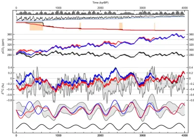
Figure 1.From top to bottom:pCO2records from Antarctic ice cores (purple: Lüthi et al., 2008); from boron isotopes in marine cores
(orange: Hönisch et al., 2009; light blue: Bartoli et al., 2011) and alkenone isotopes (pink and blue lines for the min and max envelope, from Seki et al., 2010).δ13C in cores 1143 (red: Wang et al., 2004); 849 (blue: Mix et al., 1995); 846 (green: Shackleton et al., 1995). The same δ13C records filtered at 400 kyr (bandpass=2.5 Myr−1), eccentricity (grey, from Laskar et al., 2004) and filtered eccentricity (black).
and runoff, and transforms it into a HCO−3 that finally reaches the ocean. When considering the “global” Earth surface bud-getCwhich includes the ocean and atmosphere,Whas there-fore no direct effect on C and does not appear in Eq. (1a) for dC/dt, but only as a source of alkalinity in Eq. (1b). On timescales larger than several millennia, if we assume that the oceanic calcium concentration does not change significantly over the last few millions of years, carbonate compensation will restore the oceanic carbonate content. Therefore, to first order, we can write
d[CO2−3 ]/dt=d(A−C)/dt=0=W−D−V+B.
Solving forD, this leads to the long-term evolution equation for carbon:
dC/dt=2(V−B)−W. (2a)
For simplicity, we will assume that the main stabilizer of the carbon system is the silicate weathering, with a fixed relax-ation timeτC, i.e.W=C/τC. Solving the present-day
equi-librium withδEq13=0 ‰ as a typical value for carbonates, we easily deduce typical equilibrium values for the fluxes:B0=
V /5;CEq=(8/5)τCV =40 000 PgC. If we assume a
relax-ation timeτCof 200 kyr (Archer et al., 1997), we obtainV =
(5/8)CEq/τC=125 TgC yr−1 andB0=25 TgC yr−1. For a
larger valueτC=400 kyr (Archer, 2005), we would getV =
62 TgC yr−1. There is no consensus on the actual total carbon emissions from volcanism (including all aerial and subma-rine sources), but these values forV (orτC) span more or less
the range of current estimates from about 40 to 175 TgC yr−1 (Burton et al., 2013).
It must be stressed that B stands for all organic carbon fluxes, whether they correspond to organic carbon burial (positive contributions toB) or to organic matter oxidation (negative contributions toB). While the long-term average equilibrium value B0 needs to be positive to account for
the isotopic balance as shown above, this is not necessar-ily always the case for the instantaneous values ofB, as we will illustrate in what follows with the astronomical forcing. Indeed, B represents a sum of positive and negative terms whose individual absolute magnitudes are much larger than the long-term net valueB0. For instance, the oxidation of
pet-rogenic organic carbon alone will contribute negatively toB, with a magnitude that may be as large as 40 TgC yr−1(Blair et al., 2003).
The isotopic13C budget can be written as
d/dt(Cδ13C)=V δ13V−Bδ13B−Dδ13D,
where δ13C is the isotopic composition of ocean carbon,
δ13V the isotopic composition of the volcanic carbon input,
δ13B the isotopic composition of organic matter andδ13D
the isotopic composition of marine carbonates. This can be rewritten as
or
C(dδ13C/dt)=V δ13V −Bδ13B−Dδ13D
−(V−B−D)δ13C
=V(δ13V −δ13C)−B(δ13B−δ13C)
−D(δ13D−δ13C).
If we neglect isotopic fractionation during carbonate precipi-tation (in other words,δ13D=δ13C) and more generally dur-ing carbonate compensation, we finally obtain
dδ13C/dt=(V(δ13V −δ13C)−B(δ13B−δ13C))/C. (2b) In the following we will assume a constant−5 ‰ volcanic source δ13V, as well as a constant −25 ‰ organic matter valueδ13B(e.g. Porcelli and Turekian, 2010).
In order to translate the total carbon content C into an equivalentpCO2level, we will use a simple scaling. Indeed,
if we assume, to first order, thatCmay represent the carbon content of a well-mixed ocean, then from chemical equilib-rium pCO2 should be proportional to
HCO−32/hCO2−3 i. After carbonate compensation (i.e. assuming that hCO2−3 i remains constant) and considering that C is dominated by bicarbonatesHCO−3under standard pH conditions, we end up with the approximate scaling that pCO2 varies roughly
asC2, orpCO2=280 (C/40 000)2(in ppm). To reproduce a
multi-million year trend, we need to add one explicitly in the weathering relaxation: W=C/τC=(1C+CEq−γ t)/τC,
with the coefficientγ set to 1.2 TgC yr−1to obtain the de-sired pCO2 levels at the start of the simulation, i.e. about
350 ppm at 4 Myr BP, according to current estimates (Bartoli et al., 2011; Seki et al., 2010). The model is integrated from an arbitrary initial condition at 5 Myr BP and the first 1 Myr is discarded.
In the following, we describe how carbon burial B should vary with monsoons, and what consequences these variations have on the total carbon contentC as well as on carbonate isotopesδ13C. In order to represent the monsoon’s response to astronomical forcing, we introduce a simple truncation of the precessional forcing:
F0(t)=max(0,−esinω),
whereeis the eccentricity andωthe climatic precession. Indeed, soil erosion or sediment transport are dominated by intense events, not by the average climate. Such a non-linear response can be mimicked in a simple way by the above expression that accounts only for positive monsoonal forcing, not for a negative one. Consequently, the model will be influenced by the amplitude modulation of the preces-sional forcing, i.e. the eccentricity. To avoid useless parame-ters, we furthermore introduce the normalization
F =F0/Max(F0)− hF0/Max(F0)i,
which results in a precessional forcingF(t) with amplitude 1 and 0 mean.
We implicitly account for a slow terrestrial organic carbon reservoir (soil) as “buried organic carbon”. It is reasonable to assume that monsoon or enhanced precipitation will favour primary production and soil formation. But this recent soil together with older soils and with petrogenic organic carbon (Galy et al., 2008) will be eroded and transported to the ocean through enhanced river discharges. If the corresponding car-bon is remineralized in the ocean without too much burial in the alluvial fan, the net perturbation of the burial flux is likely to be negative (i.e. net “old” soil erosion and reminer-alization). We will refer to this case as the “Amazon-like” situation, with the perturbationF(t) being subtracted to the baseline burialB0by writingB=B0−aF(t). In contrast, if
most of the organic carbon is buried and preserved in the sed-iment, then the perturbation is likely to be positive, since it induces a net “recent” soil formation and burial. We call this the “Himalayan-like” situation, with nowB=B0+aF(t).
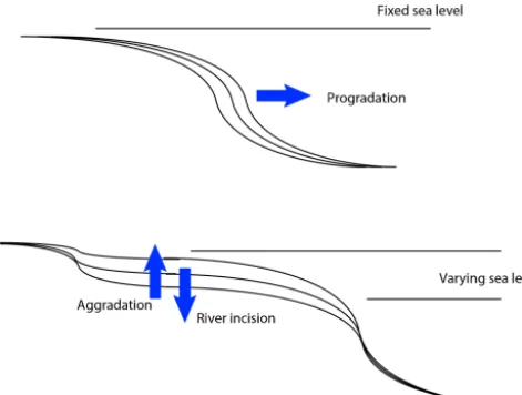
Before 1 Myr BP and the associated major sea level changes, the river fans and continental shelves should evolve mostly in a progradational way (see scheme in Fig. 3), a situation which a priori favours organic carbon remineralization, while aggradational situations are likely to be more frequent in the late Pleistocene, with therefore a possible temporary reversal of the organic carbon burial.
3 Results
Our first simulations, withB=B0−aF(t), correspond to a
perpetual “Amazon-like” situation. They correspond to ex-perimenta (black lines) with no trend in the total carbon, and experimentb(blue lines), with an explicit linear trend in carbon. The value of the parametera is chosen in order to obtain approximately the correct amplitude for these simu-lated 400 kyr oscillations (a=50 TgC yr−1). Still, as can be seen in Fig. 2, we obtain a surprisingly good match between the simulated and observed δ13C, with overall very simi-lar cycles. More specifically, theδ13C black and blue sim-ulated curves are superimposed and almost undistinguish-able, since the linear trend added to the carbon cycle has almost no impact on the δ13C. They are both most of the time within the range of observed values (grey curves). The two main exceptions occur at about 0.3 and 2.3 Myr BP, with the simulatedδ13C being significantly too high. In experi-ment a (black lines), pCO2 is oscillating around its
0 1000 2000 3000 4000 280
300 320 340 360
280 300 320 340 360
0 1000 2000 3000 4000
0.8 0.6 0.4 0.2 0 0.2 0.4
0 1000 2000 3000 4000
0.8 0.6 0.4 0.2 0 0.2 0.4
Time kyrBP
δ
13C
‰
pCO
2
ppm
Time kyrBP
δ
13C
‰
pCO
2
ppm
Figure 2.From top to bottom: precessional forcingF0(t)=Max(0,−esinω) (black line) from Laskar et al. (2004). Sea level curve LR04
(black line) from Lisiecki and Raymo (2005) used to compute the river incisionzMINdefined as the previous sea level minima (blue line). The geomorphological variablesused from experimentc(red lines) relaxed to its prescribed maximum valuesMAX∼z3MIN(black line). The orange shaded areas correspond to the aggradation regimes (i.e.s <0.85sMAX). Total carbon C rescaled aspCO2for experimentsa (black, precessional forcing only),b(blue, similar experiment but with a linear trend in carbon), andc(red, using the geomorphological dynamics from Eq. 3). Carbon isotopic compositionδ13C for experimentsa(black),b(blue), andc(red). In grey, the min and max values of the13C records from Fig. 1. The 400 kyr filtered values ofδ13C results (blue and red) together with the range of filtered records (grey). The 400 kyr filtered eccentricity as in Fig. 1. In order to obtain these results, we choseτC=200 kyr (Archer et al., 1997) or equivalently V =125 TgC yr−1. The trend (experimentsbandc) is set toγ=1.2 TgC yr−1to induce a drift from about 350 to about 280 ppm. The amplitude of the organic matter burial perturbation (experimentsa, bandc) is set toa=50 TgC yr−1. The filling rate of the sedimentary reservoir (experimentc) is set tob=(160 kyr)−1. The model is integrated from an arbitrary initial condition at 5 Myr BP and the first 1 Myr is discarded.
2.8 Myr BP, is coincident with the Plio-Pleistocene transition and the development of Northern Hemisphere glaciations. The second one near 0.8 Myr BP is coincident with the mid-Pleistocene transition (MPT) and the significant amplifica-tion of glaciaamplifica-tions. Note that the timing of these two steps is directly linked to the astronomical forcing: it does not depend at all on the specifics of the trend that we used here. Two similarpCO2 decreasing episodes are also seen in the data
(Fig. 1), though it is difficult to associate them with a pre-cise timing, due to the difficulties in accurately reconstruct-ingpCO2from indirect proxies.
In order to account for the observed departure of theδ13C oscillations from a simple eccentricity forcing, we need to introduce a retroaction of Quaternary sea level changes onto the sedimentary dynamics of alluvial fans and continental shelves, and consequently onto organic carbon burial. As ex-plained above, we will reverse the sign of our burial flux perturbation, and change it intoB=B0+aF(t) when some
conditions are met on the geomorphology of river outputs. In particular, it is necessary to account for a changing reser-voir size that can be filled with sediments in an aggradational way. Indeed, at the first major sea level drop, rivers are incis-ing though the river and fan bedrock, thus providincis-ing room for the accumulation of sediments loaded with organic carbon. This volume should be filled progressively with sedimen-tary organic carbon up to a point when further river incision, and consequent aggradation of sediment, no longer affect the global organic carbon but only move sedimentary carbon from one place to another. In other words, we will assume that the global “Himalayan-like” situation (i.e. net organic carbon burial) is only a transient situation, linked to the first occurrence of a sea level minimum. In order to illustrate this mechanism, we add a new equation for the slow geomorpho-logical reservoirS for organic carbon in river beds or river fans. We define its maximal sizeSMAX from the observed
Figure 3. Simple scheme of the two different geomorphological dynamics considered here. (top) With small sea level changes, we assume that the dominant sedimentary regime is progradation, with rather small organic carbon burial in coastal areas. The net effect of precessional forcing is (old) soil erosion, therefore a net trans-fer of carbon to the ocean–atmosphere. (bottom) With large sea level changes during the late Quaternary, the dominant sedimen-tary regime can switch temporarily to aggradation just after major sea level drops and river incisions. During these transitory phases, the net effect of precessional forcing is reversed, with net organic carbon burial in river beds and river fans.
and Raymo, 2005) by finding the previous sea level minimum
zMIN(i.e. the lower envelope) with the scalingSMAX∼z3MIN
since it represents a volume of sediment (see Fig. 2):
ifS < SMAX: dS/dt=bF0(t)
otherwise: S=SMAX. (3a)
In other words, the sedimentary organic carbon reservoirS
grows at the pace of the above-mentioned astronomical per-turbation F0(t) up to its maximal sizeSMAX. After a short
transient period, this reservoir remains therefore equal to this maximum value SMAX in the absence of major sea level
drops, as during the pre-Quaternary period. In contrast, for each significant sea level drop,SMAXincreases abruptly and
we start a new transient phase whose duration is linked to pa-rameterb. WhenSis small compared to the maximal reser-voir sizeSMAX, then the aggradational scheme is favoured,
with river beds and deltaic net organic carbon burial. But when S is close to its maximum value, we switch back to a mostly progradational sedimentation scheme, meaning that potential sea level changes will no longer affect net global organic carbon burial:
ifS <0.85SMAX: B=B0+aF(t)
otherwise: B=B0−aF(t). (3b)
Using this simple crude criterion, we obtain the results shown in Fig. 2 (experimentc, red lines). As expected, this simple
model does switch from the background “Amazon-like” or progradational burial mode to a “Himalayan-like” or aggra-dational mode, after each significant sea level drop, and most notably at two time periods, the first one between 2.4 and 2.5 Myr BP (as a consequence of the Plio-Pleistocene tran-sition) and the second and largest one between 350 and 650 kyr BP (as a consequence of the MPT). The start of these transient periods is directly linked to sea level drops, accord-ing to the LR04 forcaccord-ing, while the duration of these transients is linked both to the 0.85SMAXthreshold and theb
parame-ter, whose values are chosen to qualitatively better match the
δ13C data. For the results shown in Fig. 2,b=(160 kyr)−1. Indeed, this sedimentary switch mechanism allows for a much better agreement with measuredδ13C around 0.3 and 2.3 Myr BP, while the first simulations were systematically too high at this time, as illustrated by the difference between the blue and red curves in Fig. 2. We also simulate correctly theδ13C maximum around 500 kyr BP and the occurrence of two broad “500 kyr” cycles over the last million years. With this burial mode switching mechanism, we are also able to predict an absolute minimum in carbon content, or long-term
pCO2, around 600 kyr BP, in rather good agreement with the
long-term trend of pCO2 measured in Antarctic ice cores.
Indeed,pCO2from the Dome C record is about 5 to 10 ppm
lower before the MPT (between 400 and 800 kyr BP), which is also what we obtain in our experimentc.
4 Discussion
When variations in B, as determined by parameter a, are smaller than the baseline value B0, the model cannot
re-produce the oceanic amplitude ofδ13C observed in marine benthic records. The observed 400 kyr signal inδ13C records therefore requires major changes in the organic carbon burial, with almost no global net burial, but net oxidation episodes, during maxima of precessional forcing. This strong forcing therefore implies significant oscillations in the Earth carbon cycle for this time frequency, up to 4 or 5 % in total carbon content. This is translated here into 10 to 20 ppm variations of
pCO2using our simple scaling, but it is very likely that these
changes would be much larger, when accounting for interac-tions betweenpCO2and climate. Indeed, colder climates are
more favourable to oceanic carbon storage, as observed dur-ing the last glacial cycles. Accorddur-ing to this mechanism, in the ordinary sedimentary regime (progradation), we obtain changes in the carbon cycle withpCO2 maxima and δ13C
minima associated directly with eccentricity maxima. This is indeed consistent with long Cenozoic records (e.g. Pälike et al., 2006).
a maximum now (δ13Cmax-I), a well-marked maximum at about 500 kyr BP (δ13Cmax-II) and a previous one around 1000 or 1100 kyr BP (δ13Cmax-III). In the model described here, these two long oscillations are generated from the ec-centricity forcing, but with an abrupt switch to aggradation mode at about 620 kyr BP caused by the sea level drop at MIS 16. This switch reverses the phase of the 400 kyr car-bon oscillation during a few hundred thousands of years. In-terestingly, this also induces a slight minimum in the car-bon (or pCO2) results, consistent with the observed low
pCO2values observed in the Antarctic ice core around 600–
700 kyr BP. This mechanism also allows for simulated ma-rineδ13C in better agreement with data at about 2.4 Myr BP. It has already been noted (Wang et al., 2004) that the climatic evolution over the last million years, in particular the MPT (about 0.8 Myr BP) and the Mid-Brunhes Event (MBE, about 0.4 Myr BP) is associated with the carbon iso-topic maximaδ13Cmax-II andδ13Cmax-III. This is a strong indication of a possible causal link between the long-term well-recognized eccentricity forcing on the carbon cycle and the Plio-Pleistocene climatic evolution. There is therefore a strong incentive to build a mechanistic astronomical theory of the carbon cycle. But a prerequisite towards understanding this long-term precessionally forced carbon cycle and its cli-matic consequences is to explain the observed changes dur-ing the Quaternary, in terms ofδ13C, and simultaneously in the atmospheric CO2levels (Lüthi et al., 2008). The model
results outlined above are a first step in this direction. As detailed above, the fact that the 400 kyr carbon isotope cycle is perturbed during the Pleistocene strongly points to-wards a major role for organic matter burial over continental shelf areas being affected by sea level changes. Obviously, this model is far too simple to represent faithfully the com-plexities of sedimentary dynamics in coastal areas, its con-sequences on organic matter preservation, on carbon cycle and ultimately on climate. Furthermore, we provide here no explanation for the prescribed multi-million-year decreasing trend inpCO2. There is unfortunately no clear consensus on
the actual mechanisms involved, though this trend has been often attributed to long-term changes in continental weather-ing linked either to mountain uplift (Raymo and Ruddiman, 1992), to continental drift or mantle degassing rate (Lefeb-vre et al., 2013). Furthermore, we considered only sea level changes as a potential feedback on organic matter burial in coastal areas. Obviously, many other important climatic feed-backs would also play a role. For instance, increased tem-perature would probably reduce net primary production as a consequence of increased stratification, and therefore re-duce organic carbon deposition in coastal sediments, but it would also decrease oxygen concentrations and consequently would favour organic matter preservation. Similarly, stronger monsoon events would enhance the delivery of nutrients to the continental shelves, and therefore biological productivity. This would in addition deliver more fine-grained clay min-erals that are necessary to seal and preserve organic matter
from oxidation. This would work opposite to our continental soil–carbon mechanism for which enhanced monsoons lead to more organic carbon oxidation in agreement with the iso-topic records. But, as a proof of concept, our model is chosen as minimalistic as possible. It does not attempt to include all potentially important mechanisms.
5 Conclusion
Our basic assumptions are primarily based on recent re-assessments of riverine organic carbon inputs to the ocean. With the above conceptual model, we demonstrate that sim-ple mechanistic assumptions can account for the major pat-terns of the observed global evolution of carbon and carbon isotopes over this time period. First, enhanced precessional forcing linked to high eccentricity leads to more continen-tal organic carbon being washed out and remineralized, and therefore a net decrease in overall organic carbon burial. Sec-ond, this mechanism is temporarily reversed following ma-jor sea level drops associated with glaciations. This model was built on the premises that changes in organic matter or petrogenic organic carbon fluxes are responsible for the 400 kyr oscillations observed in Cenozoic13C records, and that the large sea level variations occurring during the Qua-ternary strongly affect this process. Continental margins and sedimentary fans are a very likely key component, as illus-trated by our simple conceptual model. But obviously, many complex processes are involved in the interactions between organic matter burial or oxidation, monsoons and sea level changes. The geomorphological mechanism described here is one possibility which allows us, for the first time, to ac-count both for the persistent 400 kyr oscillation observed in
13C records during the Cenozoic and its change during the
last million years. It also suggests the occurrence of possibly significant CO2drops at about 0.8 Myr BP (mid-Pleistocene
transition) and at about 2.8 Myr BP (Plio-Pleistocene tion), which would ultimately link the timing of these transi-tions to the astronomical forcing. Our model also provides a possible explanation for the puzzling shifted level in the CO2
records associated with the MBE.
Data availability. No data sets were used in this article.
Competing interests. The author declares that he has no conflict
of interest.
Acknowledgements. The author thanks Nathaëlle Bouttes, Peter
Köhler and the two anonymous reviewers for their useful comments and suggestions.
Edited by: Arne Winguth
References
Archer, D.: Fate of fossil fuel CO2in geologic time, J. Geophys. Res., 110, C09S05, https://doi.org/10.1029/2004JC002625, 2005.
Archer, D., Kheshgi, H., and Maier-Raimer, E.: Multiple timescales for neutralization of fossil fuel CO2, Geophys. Res. Lett., 24, 405–408, 1997.
Bartoli, G., Hönisch, B., and Zeebe, R. E.: Atmospheric CO2 decline during the Pliocene intensification of North-ern Hemisphere glaciations, Paleoceanography, 26, PA4213, https://doi.org/10.1029/2010PA002055, 2011.
Bassinot, F., Beaufort, L., Vincent, E., Labeyrie, L., Rostek, F., Müller, P., Quidelleur, X., and Lancelot, Y.: Coarse fraction fluc-tuations in pelagic carbonate sediments from the tropical In-dian Ocean: A 1500-kyr record of carbonate dissolution, Pale-oceanography, 9, 579–600, 1994.
Billups, K., Pälike, H., Channell, J., Zachos, J., and Shackleton, N.: Astronomic calibration of the late Oligocene through early Miocene geomagnetic polarity time scale, Earth Planet. Sc. Lett., 224, 33–44, 2004.
Blair, N. E., Leithold, E. L., Ford, S. T., Peeler, K. A., Holmes, J. C., and Perkey, D. W.: The persistence of memory: the fate of ancient sedimentary organic carbon in a modern sedimentary system, Geochim. Cosmochim. Ac., 67, 63–73, 2003.
Burdige, D. J.: Burial of terrestrial organic matter in marine sedi-ments: A re-assessment, Global Biogeochem. Cy., 19, GB4011, https://doi.org/10.1029/2004GB002368, 2005.
Burton, M. R., Sawyer, G. M., and Granieri, D.: Deep carbon emis-sions from volcanoes, Rev. Mineral. Geochem., 75, 323–354, 2013.
Cramer, B., Wright, J. D., Kent, D. V., and Aubry, M.-A.: Or-bital climate forcing ofδ13C excursions in the late Paleocene– early Eocene (chrons C24n–C25n), Paleoceanography, 18, 1097, https://doi.org/10.1029/2003PA000909, 2003.
Galy, V., France-Lanord, C., Beyssac, O., Faure, P., Kudrass, H., and Palhol, F.: Efficient organic carbon burial in the Bengal fan sustained by the Himalayan erosional system, Nature, 450, 407– 410, 2007.
Galy, V., Beyssac, O., France-Lanord, C., and Eglinton, T.: Recy-cling of Graphite During Himalayan Erosion: A Geological Sta-bilization of Carbon in the Crust, Science, 322, 943–945, 2008. Hilgen, F. J., Abdul Aziz, H., Krijgsman, W., Langereis, C. G.,
Lourens, L. J., Meulenkamp, J. E., Raffi, I., Steenbrink, J., Turco, E., Van Vugt, N., Wijbrans, J. R., and Zachariasse, W. J.: Present status of the astronomical (polarity) time-scale for the Mediter-ranean Late Neogene, Philos. T. R. Soc. A, 357, 1931–1947, 1999.
Hilton, R. G., Galy, V., Gaillardet, J., Dellinger, M., Bryant, C., O’Regan, M., Gröke, D. R., Coxall, H., Bouchez, J., and Calmels, D.: Erosion of organic carbon in the Arctic as a geological carbon dioxide sink, Nature, 524, 84–87, 2015.
Hönisch, B., Hemming, N. G., Archer, D., Siddall, M., and Mc-Manus, J.: Atmospheric Carbon Dioxide Concentration Across the Mid-Pleistocene Transition, Science, 324, 1551–1554, 2009. Kuiper, K. F., Deino, A., Hilgen, F. J., Krijgsman, W., Renne, P. R., and Wijbrans, J. R.: Synchronizing Rock Clocks of Earth His-tory, Science, 320, 500–504, 2008.
Laskar, J., Robutel, P., Joutel, F., Gastineau, M., and Correia, A. C. M.: A long-term numerical solution for the insola-tion quantities of the Earth, Astron. Astrophys., 428, 261–285, https://doi.org/10.1051/0004-6361:20041335, 2004.
Lefebvre, V., Donnadieu, Y., Goddéris, Y., Fluteau, F., and Hubert-Théou, L.: Was the Antarctic glaciation delayed by a high de-gassing rate during the early Cenozoic?, Earth Planet. Sc. Lett., 371–372, 203–211, 2013.
Lisiecki, L. and Raymo, M.: A Pliocene-Pleistocene stack of 57 globally distributed benthicδ18O records, Paleoceanography, 20, PA1003, https://doi.org/10.1029/2004PA001071, 2005. Lourens, L. J., Antonarakou, A., Hilgen, F. J., VanHoof, A. A. M.,
Vergnaud-Grazzini, C., and Zachariasse, W. J.: Evaluation of the Plio-Pleistocene astronomical timescale, Paleoceanography, 11, 391–413, 1996.
Lüthi, D., Le Floch, M., Bereiter, B., Blunier, T., Barnola, J.-M., Siegenthaler, U., Raynaud, D., Jouzel, J., Fisher, H., Kawamura, K., and Stocker, T.: High-resolution carbon dioxide concentra-tion record 650,000–800,000 years before present, Nature, 453, 379–382, 2008.
Mix, A. C., Pisias, N. G., Rugh, W., Wilson, J., Morey, A., and Hagelberg, T. K.: Benthic foraminifer stable isotope record from Site 849 (0–5 Ma): Local and global climate changes, Proc. Ocean Drill. Program Sci. Results, 138, 371–412, 1995. Paillard, D.: Quaternary glaciations: from observations to theories,
Quaternary Sci. Rev., 107, 11–24, 2015.
Paillard, D. and Donnadieu, Y.: A 100 Myr history of the carbon cy-cle based on the 400 kyr cycy-cle in marineδ13C benthic records, Paleoceanography, 29, https://doi.org/10.1002/2014PA002693, 2014.
Pälike, H., Norris, R. D., Herrle, J. O., Wilson, P. A., Coxall, H. K., Lear, C. H., Shackleton, N. J., Tripati, A. K., and Wade, B. S.: The heartbeat of the Oligocene climate system, Science, 314, 1894–1898, 2006.
Porcelli, D. and Turekian, K. K.: The History of Planetary De-gassing as Recorded by Noble Gases, §6.6.1 in Readings from the Treatise on Geochemistry, edited by: Holland, H. D. and Turekian, K. K., 2010.
Raymo, M. and Ruddiman, W. F.: Tectonic forcing of late cenozoic climate, Nature, 359, 117–122, 1992.
Rickaby, R., Bard, E., Sonzogni, E., Rostek, F., Beaufort, L., Barker, S., Rees, G., and Schrag, D.: Coccolith chemistry reveals secular variations in the global ocean carbon cycle?, Earth Planet. Sc. Lett., 253, 83–95, 2007.
Russon, T., Paillard, D., and Elliot, M.: Potential origins of 400–500 kyr periodicities in the ocean carbon cycle: A box model approach, Global Biogeochem. Cy., 24, GB2013, https://doi.org/10.1029/2009GB003586, 2010.
Seki, O., Foster, G. L., Schmidt, D. N., Mackensen, A., Kawamura, K., and Pancost, R. D.: Alkenone and boron-based Pliocene pCO2records, Earth Planet. Sc. Lett., 292, 201–211, 2010. Sexton, P., Norris, R. D., Wilson, P. A., Pälike, H., Westerhold, T.,
Röhl, U., Bolton, C. T., and Gibbs, S.: Eocene global warming events driven by ventilation of oceanic dissolved organic carbon, Nature, 471, 349–352, 2011.
Wang, P., Tian, J., Cheng, X., Liu, C., and Xu, J.: Major Pleistocene stages in a carbon perspective: The South China Sea record and its global comparison, Paleoceanography, 19, PA4005, https://doi.org/10.1029/2003PA000991, 2004.