www.ocean-sci.net/7/219/2011/ doi:10.5194/os-7-219-2011
© Author(s) 2011. CC Attribution 3.0 License.
Ocean Science
Multifractal analysis of oceanic chlorophyll maps remotely sensed
from space
L. de Montera1, M. Jouini1, S. Verrier2, S. Thiria1, and M. Crepon1
1Laboratoire d’Oc´eanographie et du Climat, Exp´erimentation et Approches Num´eriques, UMR 7159, Paris, France 2Laboratoire Atmosph`eres, Milieux, Observations Spatiales, UMR 8190, Guyancourt, France
Received: 14 October 2010 – Published in Ocean Sci. Discuss.: 21 January 2011 Revised: 24 March 2011 – Accepted: 25 March 2011 – Published: 28 March 2011
Abstract. Phytoplankton patchiness has been investigated with multifractal analysis techniques. We analyzed oceanic chlorophyll maps, measured by the SeaWiFS orbiting sen-sor, which are considered to be good proxies for phytoplank-ton. The study area is the Senegalo-Mauritanian upwelling region, because it has a low cloud cover and high chloro-phyll concentrations. Multifractal properties are observed, from the sub-mesoscale up to the mesoscale, and are found to be consistent with the Corssin-Obukhov scale law of pas-sive scalars. This result indicates that, in this specific region and within this scale range, turbulent mixing would be the dominant effect leading to the observed variability of phyto-plankton fields. Finally, it is shown that multifractal patchi-ness can be responsible for significant biases in the nonlinear source and sink terms involved in biogeochemical numerical models.
1 Introduction
It is sometimes argued that turbulent mixing leads to ho-mogeneous fields. However, Kolmogorov (1941), Obukhov (1949) and Corssin (1951) have shown that, on the contrary, turbulent mixing generates highly irregular structures that are heterogeneous at all scales. Their work was based on the hy-pothesis of scale invariance, which means, in simple words, that eddies can be expected to occur in a similar manner at all scales. In the case where the physical quantity is the concen-tration of a passive tracer, these authors demonstrated that its variability exhibits fractal properties which can be described
Correspondence to: S. Thiria
statistically using scale laws. This result is often referred to as the theory of passive scalars.
are dominated by turbulent mixing. This hypothesis is sup-ported by the fact that the zooplankton’s concentration power spectrum whitens at scales smaller than the “planktoscale” (Currie and Roff, 2006).
At scales larger than the “planktoscale”, the phytoplankton patchiness description is more confused. Some authors found a power spectrum slope steeper than−5/3 (around−2, Cur-rie and Roff, 2006; Seuront et al., 1999), interpreting this re-sult as a transition from Eulerian to Lagrangian statistics, due to the inertia of the boat carrying the instruments (cf. Seuront et al., 1996b). On the other hand, the analysis of remotely sensed phytoplankton fields from aircraft led to a smoother slope (around−1.2, Lovejoy et al., 2001b). From a theoreti-cal point of view, the situation is even less clear: some studies reached the conclusion that growth and trophic interactions should decrease the slope of the power spectrum (Denman and Platt, 1976; Fasham, 1978), whereas some others predict that it should increase (Steele and Henderson, 1979) or that the power spectrum has no specific regime (Horwood, 1978). In this context, to the best of our knowledge, the large volumes of data collected by remote sensing from space, over a period of more than two decades, have almost not been exploited in order to improve scientific understanding of the multi-scaling properties of phytoplankton fields (with the noticeable exception of Nieves et al., 2007). The aim of the present study is to analyze oceanic chlorophyll maps ob-tained through the use of this type of sensor. The first part of the paper briefly recalls the passive scalar theory and the no-tion of multifractal intermittency. The second and third parts describe both the cascade model and the analysis technique. The fourth part presents the dataset and the pre-treatments. The fifth and sixth parts are dedicated to the results and their interpretation. Finally, the last part of the paper provides an example of the importance of multifractal patchiness in oceanic tracers, by assessing the biases it produces in bio-geochemical numerical models.
2 Theoretical background: turbulence and multifractals
Richarsdon (1922) described turbulence as a cascade process that transfers kinetic energy from large scales to small scales by a hierarchy of imbricated eddies. The hypothesis of scale invariance relies on phenomenology and the invariance of the Navier-Stokes equations under dilatation or contraction of the reference system (see Appendix A of Schertzer and Love-joy, 1987). On the basis of this hypothesis, and the conserva-tion of energy in the inertial range, Kolmogorov (1941) used dimensionality and some general assumptions, such as ho-mogeneity and isotropy, to derive his famous statistical scale law:
1vl'ε1/3l1/3 (1)
In this equation, 1vl ≡ h|v(x+l)−v(x)|i represents the
mean shear of (longitudinal) velocity between two points separated by a distancel, andεrepresents the mean density of the energy flux, which is equal to the rate of energy dis-sipation per unit mass. A similar scale law has been derived for the concentrationC of a passive tracer (Obukhov, 1949; Corrsin, 1951):
1Cl'ϕ1/3l1/3 (2)
whereϕ≡χ3/2ε−1/2represents the non-linear coupling be-tween velocity and concentration, with χ≡ −∂(1Cl)2
∂t the
mean density of the concentration variance flux (for a review concerning these early turbulent models, see, e.g., Panchev, 1971).
Landau and Lifshitz (1944) pointed out that these fluxes have no reason to be homogeneous: although they are on av-erage conserved during the cascade process, their transfer is a priori intermittent. This remark has led the transfer process to be described by stochastic multiplicative cascades (Novikov and Stewart, 1964; Yaglom, 1966). A multiplicative cas-cade can be constructed by iterating the following simple procedure: (i) distribute a quantity uniformly over an inter-val, (ii) divide this interval into sub-intervals, (iii) multiply these by a random variable in order to obtain the new quan-tity for each sub-interval, (iv) repeat steps (ii) and (iii) until the smallest scale of the cascade is reached. The important point here is that the distribution of the random variables, re-ferred to as the multiplicative weights in the following, does not depend on the level of iteration of the construction al-gorithm. Thus, because the latter is not dependent on scale, the resulting mathematical object has fractal and even mul-tifractal properties. It turns out that these properties can be described by the scaling of its statistical moments, of frac-tional orderq(for more details, see Schertzer et al., 2002):
εlq'
L l
Kε(q)
(3)
χlq'
L l
Kχ(q)
(4) whereεl andχl are the fluxes averaged at scalel,Lis the
largest scale of the cascade, andKε(q)andKχ(q)are the
so-called moment scaling functions.
and L´evˆeque, 1994; Dubrulle, 1994) whereas some others add an assumption of self-similar renormalization, so that the generator converges more accurately towards stable distribu-tions (Schertzer and Lovejoy, 1987, 1997). Until this ques-tion finds a definitive answer, since the noques-tion of scale invari-ance is at the root of the theory, the latter assumption seems plausible, and the decision was made to use stable laws to describe the generator of the process which correspond to Gaussian distributions if the variance is finite or Levy distri-butions if the variance is infinite. In this type of case, the moment scaling functions take the simple form (Schertzer and Lovejoy, 1987):
Kε(q)=
C1ε
αε−1
qαε−q
(5)
Kχ(q)=
C1χ
αχ−1
qαχ−q
(6) whereαε and αχare multifractality parameters varying
be-tween 0 and 2, andC1ε andC1χ are intermittency
parame-ters varying between 0 and the dimension of the embedding space, which here is equal to 2.
3 The FIF model
Concerning the chlorophyll concentration, these laws can-not be directly applied, the main reason being that biologi-cal activities may produce deviations from a purely passive scalar behaviour. Nevertheless, we expect that the variability of chlorophyll maps still presents some multifractal proper-ties, and that it would be possible to use a cascade model similar to that presented above. We thus looked for a phe-nomenological model having the same form as Eq. (1), but in which the parameters are not known, i.e.:
1Chll'ζalH (7)
where Chl is the chlorophyll concentration and 1Chll≡ h|Chl(x+l)−Chl(x)|i. ζ is a conserved flux anda andH
are adjustable parameters. As described above, the conserved flux has to verify the basic multifractal relation:
ζlq'
L l
Kζ(q)
(8) and it is assumed that it converges towards a log-stable law:
Kζ(q)=
C1ζ
αζ−1
qαζ−q. (9)
This model is described by four parameters: a, H,αζ and
C1ζ. However, it is possible to reduce the number of
pa-rameters to three, since taking thea-th power ofζ in Eq. (7) is equivalent to a simple shift ofH by Kζ(a), and to the
multiplication ofC1ζ by a factoraαζ (Lavall´ee et al., 1993).
The proof uses theq-th-order structure functions of chloro-phyll maps defined by the average of the q-th power of
chlorophyll concentration variations, denoted by1Chlql ≡ h|Chl(x+l)−Chl(x)|qi. According to Eq. (7), theq-th-order structure function is equal to:
1Chlql 'ζaqlqh. (10)
By introducing Eq. (8), this equation simplifies to:
1Chlql 'lqH−Kζ(aq). (11)
Then, the term Kζ(aq)can be decomposed into
conserva-tive and non-conservaconserva-tive parts using the following identity, which can be straightforwardly derived from Eq. (9):
K(ap)=qK(a)+aαK(q). (12)
This operation yields:
1Chlql 'lq(H−K(a))−aαζKζ(q). (13)
As expected, by defining:
Kζ0(q)≡aαζK
ζ(q)
H0 ≡H−Kζ(a),
(14) one obtains the usual form of the structure function corre-sponding to the case wherea=1:
1Chlql 'lqH 0−
Kζ0(q)
. (15)
In the following, we thus use a simplified form of Eq. (7) requiring only three parameters, namely,H,αζ andC1ζ:
1Chll'ζ lH (16)
4 Analysis technique
The first step of the analysis consists in verifying the scale law given by Eq. (9), and in estimating its exponent H. This is generally performed by using the first-order struc-ture function. Since the fluxζ is assumed to be conserved in scale space, whatever the scalel,hζliis constant. Therefore, Eq. (9) reduces to:
1Chll∝lH. (17)
This equation allowsHto be estimated using the simple ex-pression:
H=logl(1Chll). (18)
The second step consists in quantifying the multifractal prop-erties of the flux, and in estimatingαζ andC1ζ. In order to
do so, it is necessary to reconstruct the cascade and therefore to retrieve the flux at the finest available scale. According to Eq. (9), this requires a fractional derivative of orderH. How-ever, a simple derivation of integer order provides a good nu-merical approximation (Lavall´ee et al., 1993), such as taking the norm of the gradient of the field:
ζlmax≈
s dChl
dx 2
+ dChl
dy 2
. (19)
Note that, since the rest of the analysis is based on the gra-dient of the field, it is crucial to work with data affected by a low level of noise. Indeed, if the noise is strong, taking the gradient of the field will result in useless, noisy fields. Therefore the finest available scale does not necessarily cor-respond to the measurement scale: it is usually necessary to perform initial averaging of the data at a larger scale, before computing the gradient, in order to suppress the noisiest of the finest scales. The cut-off scale at which the fields have to be averaged is called the “effective measurement scale” in the following. This scale is determined by computing the power spectrum, and then estimating the wave number above which it flattens out.
Once the flux has been obtained at the “effective measument scale”, the stochastic multiplicative cascade can be re-constructed by averaging (or “degrading”) the flux at larger scales. The statistical moments are then computed for vari-ous orders and scales in order to test Eq. (8). If the scaling of the statistical moments is verified,Kζ(q)can be estimated.
Finally, the parametersαζ andC1ζare obtained by
determin-ing the least squares fit to this function.
5 Dataset
Particular attention was paid to the selection of chlorophyll maps, because multifractal analysis is very sensitive to the quality of the data. As explained above, the analysis tech-nique is based on the gradient of the field. Therefore, if the
signal is too noisy, the fluctuations due to turbulence or other processes will be hidden. Moreover, the estimation of higher-order statistical moments can easily be biased by the pres-ence of a few unrealistic values in the data, such as isolated pixels having abnormally high chlorophyll concentrations.
Another difficulty is that areas below clouds or high aerosol concentrations cannot be observed, because the sen-sor cannot see the sea surface. As a consequence, chloro-phyll maps remotely sensed from space present many “holes” of different sizes (the set defined by the locations of these missing data may be fractal itself, because cloud and aerosol distributions are also fractal, see respectively Lovejoy and Schertzer, 2006 and Lilley et al., 2004). We also noticed that the values around the periphery of these “holes” were not reliable, presumably because of uncertainties in the correc-tion of the atmospheric effect. Therefore, it was chosen to study only maps which had no missing values. This type of data is of course difficult to find, because of the abundance of clouds and aerosols in the atmosphere, such that a compro-mise needed to be found between the size of the maps and the sample size.
In order to optimize this compromise, the study area was carefully chosen. The most appropriate area was found to be the Senegalo-Mauritanian upwelling region, because it nor-mally has a very low cloud cover (although this does not re-main true during the summer months, when the InterTropical Convergence Zone (ITCZ) moves north). Another reason is the presence of upwelling, which provides high chlorophyll concentrations far from the coast, due to peculiar oceanic conditions (Aristegui et al., 2004; Lathuili`ere et al., 2008). Therefore, the choice of this area reduced the measurement noise with respect to the coherent signal. Finally, the chosen location lies between 10◦N–26◦N and 14◦E–26◦E, which corresponds to the area between the Cape Verde islands and the coast of West Africa, between Mauritania and Guinea-Bissau (see Fig. 1).
Fig. 1. Geographic map of the Senegalo-Mauritanian upwelling
re-gion.
elevation angle. Therefore, only the inner part of the scans was considered, in order to limit this effect. Note also that some authors (Lovejoy et al., 2001b) recommend using di-rect analysis of marine reflectivities (level L1 product) be-cause the fields’ heterogeneity may bias chlorophyll concen-tration retrieval algorithms. Indeed, since these algorithms are generally non-linear, it is not correct to extrapolate them directly to the measurement scale which is much larger than the scale of homogeneity. However, this problem should not affect our analysis because the retrieval of chlorophyll con-centration was performed without any extrapolation in scale space (the retrieval algorithm is based on an empirical rela-tion derived from the comparison between remotely sensed marine reflectivities and in-situ chlorophyll concentrations). Moreover, working directly with marine reflectivities is dif-ficult because of its lack of physical interpretation. Actually, the only physical quantity that can be related to a theoretical scale law is the chlorophyll concentration Chl. For example, consider a non-linear relationship of the form Chl=f (R), whereR denotes a marine reflectivity. If f is non-linear, thenf−1is also non-linear. There is consequently no reason for the marine reflectivityR=f−1(Chl) to verify a scaling of the form of Eq. (9) because non-linear transformations do not generally conserve first-order structure functions.
Finally, 100 maps of 128×128 pixels of 1 km2, with a minimum of 99.5% of available data, were extracted from SeaWiFS data over a period of one year running from July 2003 to June 2004 (a sample chlorophyll map is shown in Fig. 2). The few missing data were interpolated automati-cally by computing the mean of the surroundings pixels. All selected maps were checked manually. Some maps had to be rejected because of an offset affecting some parts of the field. The origin of this offset is not known. The gradient of the maps was also checked manually, in order to detect any
20 40 60 80 100 120
20 40 60 80 100 120
km
km
0.5 1 1.5 2 2.5 3 3.5 4 mg.m−3
Fig. 2. Example of a 128 km2horizontal chlorophyll map
(resolu-tion 1 km2)extracted from the SeaWiFS local L2 product.
0 1 2 3 4 5 6 7
−5 −4.5 −4 −3.5 −3 −2.5 −2 −1.5 −1
log2(l)
log
2
(
Δ
Chl
l
)
(1 km) (2 km) (4 km) (8 km) (16 km) (32 km) (64 km) (128 km)
Fig. 3. First-order structure function of SeaWiFS chlorophyll maps
compared with a linear curve of slope equal to 0.4. The depar-ture from the theorical fit observed at the finest scales is attributed to measurement noise, and corresponds to flattening of the power spectra at high wave numbers (see Fig. 4).
isolated, unrealistically high values. Each of these unrealistic pixels was corrected using the mean value of the surrounding pixels.
6 Results
0 1 2 3 4 5 6 14
16 18 20 22 24
log2(k)
log
2
(E
(k))
(8 km) (16 km)
(128 km) (64 km) (32 km) (4 km) (2 km)
Fig. 4. Angle-integrated power spectrum of SeaWiFS chlorophyll
maps compared with a linear curve of slope equal to−1.67. The
power spectrum flattens out at the fifth octave, corresponding to wavelengths smaller than 4 km.
because such a break in the scaling has never been observed in other studies (cf. Lovejoy et al., 2001b). This break was therefore associated with the scale below which the measure-ment noise becomes dominant, when compared with the co-herent signal (here, the definition of the noise is very large: it includes not only the sensor’s sensitivity, but also atmo-spheric corrections and retrieval algorithms errors). This hy-pothesis is confirmed by the power spectrum (Fig. 4), which flattens out beyond a wave number corresponding to 4 km in the physical space. Finally, over the scale range 4–128 km, the empirical first-order structure function is consistent with Eq. (17), andH is estimated to be around 0.4 (the numeri-cal fit yields 0.402 with a standard deviation of the estimator equal to 0.005).
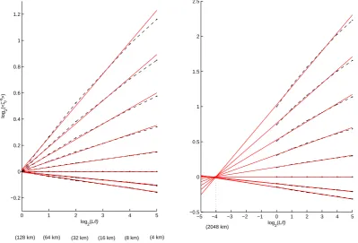
Since the noise has to be removed before continuing the analysis, the data were averaged over 4×4 km2areas. Then, for each map, the norm of the gradient was computed and normalized in order to reconstruct the cascade. Figure 5 (left) shows the scaling of the statistical moments for various or-ders. This set of scale laws is found to be consistent with the basic multifractal relation given by Eq. (8). For each orderq, the slope of the scale law provides an estimation of Kζ(q). The moment scaling function retrieved by this
method is shown in Fig. 6. The fit of this function accord-ing to Eq. (9) yieldsC1ζ≈0.12 andαζ≈1.92 (here, we
re-nounced to provide the standard deviations of the estimators because they would indicate an artificially high precision; the estimation error of the whole analysis technique has been tested with simulations and is found to be around 10% for
both parameters). Note that the values of these parameters, as well as that ofH, are close to those obtained for rain and clouds, which are respectivelyH≈0.4, C1≈0.12,α≈1.8 (Verrier et al., 2010) andH≈0.4,C1≈0.08,α≈1.9 (Love-joy and Schertzer, 2006). Another possibility is to normalize the norm of the gradient in the same manner for all maps by using the “climatological” mean computed over all maps. This technique has the advantage to provide an estimation of the outer scale of the cascade by extrapolating the scale laws of the moments (see, e.g., Lovejoy and Schertzer, 2006). Al-though the sample used in this study is limited and may not be representative, the results are presented in Fig. 5 (right) and yield an outer scale equal to 2000 km, which could be related to the size of oceanic gyres in terms of order of mag-nitude.
We also tried to perform the same type of analysis using SST (Sea Surface Temperature), which is another useful, re-motely sensed oceanic tracer. However, this attempt failed because the spectrum of the SST maps was found to flatten out at larger scales (around 32 km) than that of chlorophyll maps, and the available range of scales was thus insufficient. This whitening effect, which hides the small scale fluctua-tions, may be due to air-sea exchanges, which tend to spa-tially homogenize the SST. However, Nieves et al. (2007) performed a multi-scale analysis of SST data with a larger scale range (level L3 product) and found that the observed multifractal spectra was very similar to the one obtained with chlorophyll concentration data. This result provides an addi-tional argument in favour of a link between phytoplankton patchiness and turbulent mixing at large scales, which will be developed in the next section.
0 1 2 3 4 5 −0.2
0 0.2 0.4 0.6 0.8 1 1.2
log2(L/l)
log
2
(<
ζl q>)
−5 −4 −3 −2 −1 0 1 2 3 4 5 −0.5
0 0.5 1 1.5 2 2.5
log2(L/l)
(8 km) (16 km) (32 km) (64 km)
(128 km) (4 km)
(2048 km)
Fig. 5. Scaling of the statistical moments of the fluxζ for the ordersq=0, 0.1, 0.2, . . . , 2, with corresponding theoretical fits. Here,L corresponds to the largest scale of the SeaWiFS chlorophyll maps, i.e. 128 km. Left: for each map, the flux was normalized to a mean value of 1. Right: the normalization was performed with the “climatological” mean value computed over all maps, which allows estimating the outer scale of the cascade by extrapolation to larger scales.
0 0.5 1 1.5 2
−0.05 0 0.05 0.1 0.15 0.2 0.25 0.3
q
Kζ
(q
)
Fig. 6. Moment scaling functionKζ(q)of the fluxζ, with theoreti-cal fit.
be estimated using a different approach, since the theoretical slope of the asymptote this distribution is equal to−(1+α). The resulting value ofαis found to be 1.95, which is consis-tent with the value previously obtained using statistical mo-ments.
7 Interpretation
Since the parameterH was found to be close to 1/3, it is tempting to relate it to the theory of passive scalars. This theory is based on the hypothesis of a 3-D isotropic tur-bulence that does not hold for our selection of chlorophyll maps, because, in the considered scale range (1–128 km), the ocean is a stratified fluid with a horizontal dimension much larger than the vertical one. However, some recent studies (e.g., Lovejoy and Schertzer, 2010) suggest that the Corrsin-Obukhov scale law may still be valid in the horizon-tal. Therefore, if turbulent mixing is the dominant effect, we may expect that the horizontal variability of phytoplankton fields would verify the scale law given in Eq. (2). If this is correct, then, assuming the velocity and passive scalar fluc-tuations to be independent, Schmitt et al. (1996) have shown that the parameter H of the FIF model (Eq. 9) should be equal to:
H=1/3+Kε(1/6)−Kχ(1/2). (20)
The deviation ofHwith respect to the value 1/3 is due to the intermittency of the energy and scalar variance fluxes, since a conserved flux raised to a power exponent, not equal to 1, is no longer a conserved quantity. The termKε(1/6) depends
−2 −1.5 −1 −0.5 0 0.5 1 1.5 2 0
0.2 0.4 0.6 0.8 1 1.2
Logarithm of multiplicative weights
Fig. 7. PDFs of the logarithm of the multiplicative weights for each
level of the cascade (corresponding to contractions of the averaging
area by a factor 22, from 128 km2until 4 km2). The PDFs are very
similar, with the exception of the function corresponding to the last
scale contraction (from 8 km2to 4 km2), which is flatter. This may
be due to the presence of noise.
parametersαε=1.5 andC1ε=0.25 proposed by Schmitt et
al. (1996), its value is expected to be around−0.05. How-ever, the estimation of the term Kχ(1/2) is more delicate,
since the multifractal parameters ofχare not known a priori, and have to be estimated. One possible solution consists in using the empirical multifractal parameters obtained forζ in the previous section, because they have a simple approximate relationship to those ofχ(de Montera et al., 2010):
αχ ≈αζ
C1χ ≈2αζ C1ζ.
(21) This yields αχ ≈1.92 and C1χ ≈0.45, thus allowing
Kχ(1/2) to be estimated at a value equal to −0.11. The
(semi-)theoretical value ofHis therefore 1/3−0.05+0.11≈
0.39, which is consistent with its experimental value of 0.4 obtained with the SeaWiFS chlorophyll maps.
This coherency led us to the conclusion that phytoplankton behaves like a passive scalar within the studied scale range, which includes the mesoscale and the sub-mesoscale. This does not mean that phytoplankton is a purely passive scalar, however it implies that biological activity does not affect the scale law generated by turbulent mixing. This is consistent with the previous finding of Seuront et al. (1999) and Cur-rie and Roff (2006), who showed that biological activity af-fected the scaling over a limited range only, between 30 m and 500 m, which is smaller than the resolution of remotely sensed satellite data.
However, as explained in the introduction, other studies (e.g., Lovejoy et al., 2001b) found a parameter H equal
−1.2 −1 −0.8 −0.6 −0.4 −0.2 0
−8 −6 −4 −2 0 2 4 6 8 10
log(logarithm of multiplicative weights)
log(total PDF)
Fig. 8. Log-log graph of the left tail of the total PDF of the
log-arithm of multiplicative weights (blue), compared with a Gaussian having the same mean and variance (red). The PDF decays as a
power law, with a slope−2.95 (green fit), corresponding to a L´evy
law of indexα=1.95. The Gaussian function decays much faster,
and would therefore be inappropriate for cascade generation.
to 0.12 and concluded to a combined turbulent/growth-dominated process. Therefore, the question is still open and future studies should try to understand precisely in which particular seasons or locations this departure from the tur-bulent scaling is likely to occur. According to the model pro-posed in Lovejoy et al. (2001a), this departure should be ob-served in area which have a weak turbulent activity combined with a high growth rate.
8 Bias in biogeochemical numerical models
0 20 40 60 80 100 0
0.005 0.01 0.015 0.02 0.025 0.03 0.035 0.04 0.045 0.05
% of error
Fig. 9. Assessment of the distribution of the relative error
percent-age resulting from the hypothesis of homogeneity over 128 km2
areas, for a quadratic source term in a biogeochemical numerical model.
to be demonstrated (for a test of the Boussinesq hypothesis, see Schmitt, 2007).
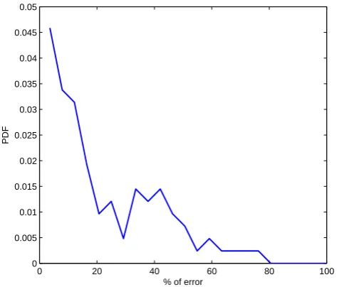
If biogeochemical processes are involved, the situation is even worse, because the estimation of these interactions is also affected by the truncation error. Moreover, the parame-ters of biogeochemical models are often obtained by means of laboratory experiments performed at a typical scale of one meter. Therefore, since the relations in which these param-eters are involved are generally non-linear, it is not correct to use them at larger scales if the real fields are heteroge-neous. It can thus be useful to assess the bias generated by the assumption of homogeneity over larger scales. For this, we consider a global numerical model operating with a 1◦grid scale (roughly corresponding to the 128 km2maps analyzed in the present paper), which includes a quadratic source term of the formβC2, whereC is the concentration of a tracer andβis a parameter assumed to be derived under stable conditions, at the scale of one meter in a laboratory. If it is assumed that the 100 SeaWiFS chlorophyll maps are realizations of the sub-grid heterogeneity of the tracer, then for each map we compute the source term at the finest avail-able scale (which is 1 km in this case, whereas a 1 m scale would be needed!), and average these values over the whole 128 km2map. Finally, we estimate the value of this source term that would result from the hypothesis of homogeneity, by averaging the concentration over the whole 128 km2map and then computing the source term. The source term is then estimated with a relative errorEequal to:
E=
Chl2
− hChli2
Chl2 . (22)
The PDF of the percentage of this relative error is shown in Fig. 9. Its mean value is approximately 22%, which is far from being negligible. One possible approach for reducing this error would be to derive an analytic expression for the scale dependency of the biological parameters (such asβ in the example above), using the multifractal parameters of the tracer patchiness, if available.
9 Conclusions
Multifractal properties of oceanic chlorophyll maps have been investigated with remotely sensed data recorded from space. The FIF model has been validated, showing that chlorophyll maps can be modelled statistically, through the use of a fractionally integrated multiplicative cascade. In the study area, the Senegalo-Mauritanian upwelling region, the parameters of this model were found to be H≈0.4,
C1≈0.12 andα≈1.92. The estimates of the scale law expo-nentHis consistent with passive scalar behaviour, indicating that phytoplankton variability is dominated by turbulent mix-ing over the studied scale range (4–128 km), and that biolog-ical activity do not modify this scaling. This result confirms previous studies that reached this conclusion based on in-situ data. However, it cannot be generalized to other locations because it may not be correct in areas having a high growth rate combined with a weak turbulent activity.
Finally, it has been shown that, as a consequence of this multifractal patchiness, the non-linear source and sink of bio-geochemical numerical models could be strongly biased. Fu-ture studies should therefore be dedicated to the use multi-fractal techniques to improve the accuracy of numerical sim-ulations. This could be performed, for example, by predict-ing the scale dependence of the model parameters or by re-fining the assimilation of data measured at different scales. Although the effect of grazing was not observed in this study because of the low resolution of satellite data, the develop-ment of such techniques implies to take it into account since the scaling is modified at lower scales, in particular at scales of the order of the so-called “planktoscale”.
Acknowledgements. This study was funded by the French Centre
National d’ ´Etudes Spatiales (CNES).
Edited by: E. J. M. Delhez
References
Aristegui, J., Alvarez-Salgado, X. A., Barton, E. D., Figueiras, F. G., Hernandez-Leon, S., Roy, C., and Santos, A. M. P.: Oceanog-raphy and fisheries of the Canary current/Iberian Region of the eastern North Atlantic, in: The Sea, Vol. 14, Chap. 23, edited by: Robinson, A. R. and Brink, K. H., John Wiley and Sons, New York, 877–931, 2004.
Corrsin, S.: On the spectrum of isotropic temperature fluctuations in an isotropic turbulence, J. Appl. Phys., 22, 469–475, 1951. Currie, W. J. S. and Roff, J. C.: Plankton are not Passive
Trac-ers: Plankton in a Turbulent Environment, J. Geophys. Res., 111, C05S07, doi:10.1029/2005JC002967, 2006.
de Montera, L., Verrier, S., Mallet, C., and Barth`es, L.: A passive scalar-like model for rain applicable up to storm scale, Atmos. Res., 98(1), 140–147, 2010.
Denman, K. L. and Platt, T.: The variance spectrum of phytoplank-ton in a turbulent ocean, J. Mar. Res., 34, 593–601, 1976. Dubrulle, B.: Intermittency in fully developed turbulence:
Log-Poisson statistics and generalized scale-covariance, Phys. Rev. Lett., 73, 959–963, 1994.
Fasham, M. J. R.: The application of some stochastic processes tothe study of plankton patchiness, in: Spatial Pattern in Plankton Communities, edited by: Steele, J. H., Springer, New York, 131– 156, 1978.
Horwood, J. W.: Observations on spatial heterogeneity of surface chlorophyll in one and two dimensions, J. Mar. Biol. Assoc. UK, 58, 487–502, 1978.
Kolmogorov, A. N.: Local structure of turbulence in an incompress-ible liquid for very large Reynolds numbers, Proc. Acad. Sci. URSS., Geochem. Section, 30, 299–303, 1941.
Landau, L. D. and Lifshitz, E. M.: Fluid mechanics, 1st edn., Edt. MIR, Moscow, 1944.
Lathuili`ere, C., Echevin, V., and Levy, M.: Seasonal and
intraseasonal surface chlorophyll-a variability along the
northwest African coast, J. Geophys. Res, 113, C05007, doi:10.1029/2007JC004433, 2008.
Lavall´ee, D., Lovejoy, S., Schertzer, D., and Ladoy, P.: Nonlinear variability and landscape topography: analysis and simulation, in: Fractals in geography, edited by: de Cola, L. and Lam, N., Prentice-Hall, 171–205, 1993.
Lilley, M., Lovejoy, S., Strawbridge, K., and Schertzer, D.: 23/9 dimensional anisotropic scaling of passive admixtures using lidar aerosol data, Phys. Rev. E, 70, 036301–036307, 2004.
Lovejoy, S. and Schertzer, D.: Towards a new synthesis for atmo-spheric dynamics: space-time cascades, Atmos. Res., 96(1), 1– 52, 2010.
Lovejoy, S. and Schertzer, D.: Multifractals, cloud radiances and rain, J. Hydrol., 322, 59–88, 2006.
Lovejoy, S., Currie, W. J. S., Tessier, Y., Claereboudt, M. R., Roff, J. C., Bourget, E., and Schertzer, D.: Universal Multifractals and ocean patchiness: phytoplankton, physical fields and coastal het-erogeneity, J. Plankton Res., 23, 117–141, 2001a.
Lovejoy, S., Schertzer, D., Tessier, Y., and Gaonac’h, H.: Multifrac-tals and Resolution independent remote sensing algorithms: the example of ocean colour, Int. J. Remote Sens., 22, 1191–1234, 2001b.
Nieves, V., Llebot, C., Turiel, A., Sol´e, J., Garc´ıa-Ladona, E., Estrada, M., and Blasco, D.: Common turbulent signature in sea surface temperature and chlorophyll maps, Geophys. Res. Lett.,
34, L23602, doi:10.1029/2007GL030823, 2007.
Novikov, E. A. and Stewart, R.: Intermittency of turbulence and spectrum of fluctuations in energy-disspation, Izv. Akad. Nauk. SSSR, Ser. Geofiz., 3, 408–412, 1964.
Obukhov, A.: Structure of the temperature field in a turbulent flow, Izv. Akad. Nauk SSSR, 13, 55–69, 1949.
Panchev, S.: Random Functions and Turbulence, Pergamon Press, London, 1971.
Pecknold, S., Lovejoy, S., Schertzer, D., Hooge, C., and Malouin, J. F.: The simulation of universal multifractals, in: Cellular Au-tomata: Prospects in astrophysical applications, edited by: Per-dang, J. M. and Lejeune, A., World Scientific, 228–267, 1993. Platt, T.: Local phytoplankton abundance and turbulence, Deep-Sea
Res., 19, 183–187, 1972.
Pottier, C., Turiel, A., and Garc¸on, V.: Inferring missing data in satellite chlorophyll maps using turbulent cascading, Remote Sens. Environ., 112, 4242–4260, 2008.
Richardson, L. F.: Weather prediction by numerical processes, Cambridge University Press, Cambridge, 1922.
Schertzer, D. and Lovejoy S.: Physically based rain and cloud mod-eling by anisotropic, multiplicative turbulent cascades, J. Geo-phys. Res., 92, 9692–9714, 1987.
Schertzer, D. and Lovejoy, S.: Universal Multifractals do Exist!, J. Appl. Meteorol., 36, 1296–1303, 1997.
Schertzer, D., Lovejoy, S., and Hubert, P.: An Introduction to Stochastic Multifractal Fields, in: ISFMA Symposium on En-vironmental Science and Engineering with related Mathematical Problems, edited by: Ern, A. and Weiping, L., Higher Education Press, Beijing, 106–179, 2002.
Schmitt, F., Schertzer, D., Lovejoy, S., and Brunet, G.: Multifractal temperature and flux of temperature variance in fully developed turbulence, Europhys. Lett., 34, 195–200, 1996.
Schmitt, F. G.: About Boussinesq’s turbulent viscosity hypothesis: historical remarks and a direct evaluation of its validity, C.R. Mecanique, 335, 617–627, 2007.
Seuront, L., Schmitt, F. G., Lagadeuc, Y., Schertzer, D., Lovejoy, S., and Frontier, S.: Universal Multifractal structure of phytoplank-ton biomass and temperature in the ocean, Geophys. Res. Lett., 23, 3591–3594, 1996a.
Seuront, L., Schmitt, F. G., Schertzer, D., Lagadeuc, Y., and Love-joy, S.: Multifractal Analysis of Eulerian and Lagrangian Vari-ability of Physical and Biological Fields in the Ocean, Nonlinear Proc. Geoph., 3, 236–246, 1996b.
Seuront, L., Schmitt, F. G., Lagadeuc, Y., Schertzer, D., and Love-joy, S.: Universal Multifractal analysis as a tool to characterize multiscale intermittent patterns: example of phytoplankton dis-tribution in turbulent coastal waters, J. Plankton Res., 21, 877– 922, 1999.
Seuront, L. and Schmitt, F. G.: Eulerian and Lagrangian properties of biophysical intermittency in the ocean, Geophys. Res. Lett., 31, L03306, doi:10.1029/2003GL018185, 2004.
Seuront, L. and Schmitt, F. G.: Multiscaling statistical procedures for the exploration of biophysical couplings in intermittent tur-bulence; Part I. Theory, Deep-Sea Res. Pt. II, 52, 1308–1324, 2005a.
Steele, J. H. and Henderson, E. W.: Spatial patterns in North Sea plankton, Deep-Sea Res., 26, 955–963, 1979.
She, Z.-S. and L´evˆeque, E.: Universal scaling laws in fully-developed turbulence, Phys. Rev. Lett., 72, 336–339, 1994. Verrier, S., de Montera, L., Barth`es, L., and Mallet, C.: Multifractal
analysis of African monsoon rain fields, taking into account the zero rain-rate problem, J. Hydrol., 389(1–2), 111–120, 2010.