Generating a series of fine spatial and temporal resolution land cover maps by fusing coarse spatial resolution remotely sensed images and fine spatial resolution land cover maps

1

Generating a series of fine spatial and temporal resolution

land cover maps by fusing coarse spatial resolution remotely

sensed images and fine spatial resolution land cover maps

4

Xiaodong Li

_{, Feng Ling}

_{*, Giles M. Foody}

_{, Yong Ge}

_{, Yihang Zhang}

_,

5

Yun Du

7

a _{Key Laboratory of Monitoring and Estimate for Environment and Disaster of Hubei}

8

Province, Institute of Geodesy and Geophysics, Chinese Academy of Sciences, Wuhan 9

430077, China 10

b _{School of Geography, University of Nottingham, University Park, Nottingham NG7}

11

2RD, U.K. 12

c _{State Key Laboratory of Resources and Environmental Information System, Institute}

13

of Geographic Sciences & Natural Resources Research, Chinese Academy of Sciences, 14

Beijing 100101, China 15

16

*Corresponding author at Key Laboratory of Monitoring and Estimate for Environment 17

and Disaster of Hubei Province, Institute of Geodesy and Geophysics, Chinese 18

Academy of Sciences, Wuhan 430077, China 19

2

ABSTRACT 21

Studies of land cover dynamics would benefit greatly from the generation of land 22

cover maps at both fine spatial and temporal resolutions. Fine spatial resolution images 23

are usually acquired relatively infrequently, whereas coarse spatial resolution images 24

may be acquired with a high repetition rate but may not capture the spatial detail of the 25

land cover mosaic of the region of interest. Traditional image spatial–temporal fusion 26

methods focus on the blending of pixel spectra reflectance values and do not directly 27

provide land cover maps or information on land cover dynamics. In this research, a 28

novel Spatial–Temporal remotely sensed Images and land cover Maps Fusion Model 29

(STIMFM) is proposed to produce land cover maps at both fine spatial and temporal 30

resolutions using a series of coarse spatial resolution images together with a few fine 31

spatial resolution land cover maps that pre- and post-date the series of coarse spatial 32

resolution images. STIMFM integrates both the spatial and temporal dependences of 33

fine spatial resolution pixels and outputs a series of fine spatial–temporal resolution 34

land cover maps instead of reflectance images, which can be used directly for studies 35

of land cover dynamics. Here, three experiments based on simulated and real remotely 36

sensed images were undertaken to evaluate the STIMFM for studies of land cover 37

change. These experiments included comparative assessment of methods based on 38

single-date image such as the super-resolution approaches (e.g., pixel swapping-based 39

super-resolution mapping) and the state-of-the-art spatial–temporal fusion approach 40

that used the Enhanced Spatial and Temporal Adaptive Reflectance Fusion Model 41

3

the fine-resolution images, in which the maximum likelihood classifier and the 43

automated land cover updating approach based on integrated change detection and 44

classification methodwere then applied to generate the fine-resolution land cover maps.

45

Results show that the methods based on single-date image failed to predict the pixels 46

of changed and unchanged land cover with high accuracy. The land cover maps that 47

were obtained by classification of the reflectance images outputted from ESTARFM 48

and FSDAF contained substantial misclassification, and the classification accuracy was 49

lower for pixels of changed land cover than for pixels of unchanged land cover. In 50

addition, STIMFM predicted fine spatial–temporal resolution land cover maps from a 51

series of Landsat images and a few Google Earth images, to which ESTARFM and 52

FSDAF that require correlation in reflectance bands in coarse and fine images cannot 53

be applied. Notably, STIMFM generated higher accuracy for pixels of both changed 54

and unchanged land cover in comparison with other methods. 55

4

1. Introduction

Land cover maps are one of the most fundamental datasets used in many scientific 58

fields and are often produced from remotely sensed images (Bartholome and Belward 59

2005; Friedl et al. 2002). A wide variety of remote sensing systems have been 60

developed, and hence, images are available with different spatial and temporal 61

resolutions, thereby allowing the production of land cover maps at different spatial and 62

temporal scales. With most satellite remote sensing systems, a trade-off typically exists 63

between spatial and temporal resolution. In general, fine spatial resolution remote 64

sensors can acquire images that provide spatially detailed land cover information, but 65

their relatively coarse temporal resolution limits their usage in monitoring rapid land 66

cover changes. By contrast, coarse spatial resolution remotely sensed images can often 67

be acquired at a fine temporal resolution that provides a repetition rate suitable for the 68

detection of rapid land cover changes but are unable to represent the spatial detail of 69

the land cover mosaic. To realize the full potential of remote sensing as a source of 70

information on land cover change, a method that allows the production of land cover 71

maps with both fine spatial and temporal resolutions is required. Such maps could be 72

obtained by combining all available remotely sensed images of varying spatial and 73

temporal resolution to form a series of fine-resolution land cover maps. 74

Recently, spatial–temporal image fusion, which aims to produce fine spatial and 75

temporal resolution remotely sensed images from images with different spatial and 76

temporal resolutions, has become a promising means to address the trade-off between 77

5

Spatial–temporal data fusion methods can be categorized into weighted function based 79

methods, unmixing-based methods, and dictionary-pair learning based methods (Zhu 80

et al. 2016). Among the weighted function based methods, the Spatial and Temporal 81

Adaptive Reflectance Fusion Model (STARFM) proposed by Gao et al. (2006) was 82

developed first and is one of the most popular spatial–temporal image fusion methods. 83

By fusing coarse spatial resolution Moderate Resolution Imaging Spectroradiometer 84

(MODIS) and fine spatial resolution Landsat sensor images, STARFM can predict 85

Landsat-like reflectance images with the spatial resolution of Landsat and the temporal 86

resolution of MODIS. A number of studies have suggested improvements to STARFM, 87

including studies of forest disturbance (Hilker et al. 2009a), and in heterogeneous 88

regions (Zhu et al. 2010), as well as in gap filling to reduce the negative effects of cloud 89

(Gevaert and Garcia-Haro 2015). STARFM and the improved models based on it have 90

been mainly used to detect reflectance changes caused by processes such as phenology 91

over large areas, and used to generate dense time series of Landsat-like data (Hilker et 92

al. 2009b), enhance land cover classification (Jia et al. 2014), and predict key 93

environmental variations such as evapotranspiration (Anderson et al. 2011) and 94

temperature (Hilker et al. 2009b). Other spatial–temporal image fusion models, such as 95

the unmixing-based algorithm that extracts endmembers on the basis of linear spectral 96

mixture model and assigns the unmixed reflectance to fine spatial resolution pixels 97

(Huang and Zhang 2014; Zhukov et al. 1999; Zurita-Milla et al. 2009) and the 98

dictionary-pair learning based methods, which capture features from the coarse- and 99

6

2012), have also been proposed and applied to Landsat and MODIS images in recent 101

years (Amoros-Lopez et al. 2013; Wu et al. 2012). 102

Generally, spatial–temporal image fusion models aim to generate a series of 103

continuous reflectance values instead of discrete categorical values. A further image 104

classification step is needed to produce from the reflectance images a corresponding 105

series of land cover maps for the study of land cover class dynamics (Jia et al. 2014). 106

The use of these methods for generating land cover maps and monitoring land cover 107

changes often suffers from two important limitations. 108

First, most spatial–temporal image fusion algorithms assume that land cover type 109

does not change during the data observation period (Fu et al. 2013; Gao et al. 2006; 110

Zhu et al. 2010). Previous research has shown that STARFM does not deal well with 111

abrupt land cover changes. Song and Huang (2013) showed that STARFM failed to fuse 112

the pixel reflectance accurately in a study of land cover change in an urban area. The 113

Enhanced STARFM (ESTARFM) is often better than STARFM for studies of 114

heterogeneous landscapes (Zhu et al. 2010) but can be worse than STARFM for 115

predicting abrupt changes of land cover type (Emelyanova et al. 2013). The Spatial 116

Temporal Adaptive Algorithm for mapping Reflectance CHange (STAARCH) 117

improves STARFM’s performance when land cover type change and disturbance exist, 118

but it is more suitable for spatial–temporal fusion of forest land cover (Hilker et al. 119

2009a). The Flexible Spatiotemporal DAta Fusion model (FSDAF) can predict 120

Landsat-like reflectance values with both gradual change and land cover type change, 121

7

pixels experienced land cover type change and the change is invisible in the coarse-123

resolution image (Zhu et al. 2016). Similar to STARFM, the unmixing-based spatial– 124

temporal reflectance fusion methods consider only the change in endmember spectra 125

but not in land cover types (Huang and Zhang 2014; Zhukov et al. 1999; Zurita-Milla 126

et al. 2009). 127

Second, most spatial–temporal image fusion methods need one or more observed 128

pairs of coarse- and resolution images for training and require the coarse- and fine-129

resolution remotely sensed data from different satellite sensors to be mutually 130

comparable and correlated. All the weighted function based methods, including 131

STARFM, ESTARFM, STAARCH, and all the dictionary-pair learning-based methods 132

need one or more observed pairs of coarse- and fine-resolution images, which have 133

comparable reflectance bands, for training (Gao et al. 2006; Gevaert and Garcia-Haro 134

2015; Zhu et al. 2010). These methods mainly focus on predicting Landsat-like 135

remotely sensed images with MODIS repetition rates. However, these methods cannot 136

deal with other satellite images, which have uncorrelated reflectance bands, and are 137

thus limited in the use of land cover change analysis. For instance, in regional-scale 138

land cover analysis, the detection of very-high-resolution land cover changes at high 139

temporal resolutions is required. In general, we can obtain a series of Landsat images 140

and a few very-high-resolution images such as panchromatic aerial photograph. The 141

weighted function based and dictionary-pair learning based methods cannot fuse these 142

data because the very-high-resolution images usually have different reflectance bands 143

8

The spatial–temporal image fusion methods aim to produce fine spatial–temporal 145

resolution reflectance images rather than land cover maps. The fused fine-resolution 146

images have many applications, such as phenology analysis. If the aim is to generate a 147

sequence of land cover maps from the reflectance images from which land cover change 148

trajectories may be extracted, then a further image classification analysis is still required, 149

which may introduce uncertainty and error in the land cover maps. First, the 150

classification of an image series can be complex and laborious. Training statistics are 151

required to inform classification analysis, and these may vary in quality in time due to 152

issues such as phenology. Moreover, the classification is also problematic, with the 153

potential for different classifiers to generate dissimilar land cover maps from the same 154

training data. Traditional classifiers applied to mono-temporal image may also ignore 155

the temporal information contained in a series of images and thereby produce a 156

classification of sub-optimal accuracy. The spatial–temporal–based image classifier has 157

the advantage in taking both the spatial and temporal links between neighboring pixels 158

(Cai et al. 2014), but is challenging to use for voluminous image series (Liu and Cai 159

2012; Liu et al. 2006). Finally, the spatial–temporal image fusion models generate a 160

large volume of fine spatial–temporal resolution reflectance images as the intermediate 161

data to be used for the production of land cover maps. This situation may represent 162

practical challenges in terms of data access and storage. 163

Given the concerns with the spatial–temporal reflectance fusion model for 164

producing land cover maps, a more appropriate fusion approach could be based on 165

9

land cover maps rather than reflectance images, with the aid of information derived 167

from a few fine spatial resolution images that may be available. Chen et al. (2015) 168

updated land cover maps from downscaled Normalized Difference Vegetation Index 169

(NDVI) time-series data from MODIS, a current Landsat image, and a Landsat image 170

that pre-dates it. The NDVI time-series data are used as ancillary data to extract changed 171

pixels in the Landsat images, and the labels of changed pixels are determined using the 172

current Landsat image. Thus, this method can update fine-resolution land cover maps 173

with Landsat repetition rates based on available Landsat images, but cannot predict 174

fine-resolution land cover maps with MODIS repetition rates. In addition, a major 175

problem with this approach is that a large proportion of coarse spatial resolution image 176

pixels may be of mixed land cover composition. A possible solution of this problem is 177

to use the fractional land cover class composition images that can be extracted via a 178

spectral unmixing analysis. A comparison of the obtained fraction images indicates the 179

change, if any, in land cover that has occurred in the time period between the dates of 180

image acquisition (Lu et al. 2004). This approach can potentially reveal important 181

temporal land cover information, such as land cover modification and conversion 182

(Foody 1999; Lu et al. 2011). Unfortunately, these approaches show only the change in 183

the fraction of the area that is represented by each coarse-resolution pixel and not the 184

geographical location of the change. Information on the location of change might be 185

obtained through a super-resolution analysis (Li et al. 2016; Wang et al. 2015). 186

Super-resolution land cover mapping (SRM) is a promising technique used to 187

10

typically viewed as a post-processing approach applied after a spectral unmixing 189

analysis. SRM predicts the spatial distribution of each land cover class in the area 190

represented by each coarse spatial resolution pixel and provides more fine spatial 191

resolution land cover information than spectral unmixing (Atkinson 2009). Various 192

approaches have been proposed (Atkinson 2005; Ge et al. 2016; Kasetkasem et al. 2005; 193

Ling et al. 2016; Tatem et al. 2003), and SRM has been used in many fields, including 194

the extraction of waterlines (Foody et al. 2005), rural land cover (Tatem et al. 2003), 195

refining the estimation of ground control point location (Foody 2002), land cover 196

change detection (Wang et al. 2015), land cover map updating (Li et al. 2015b), and 197

wetland inundation analysis (Li et al. 2015a). 198

Traditionally, SRM is applied to a mono-temporal coarse spatial resolution image 199

dataset. The SRM solution space is large because SRM predicts land cover maps with 200

finer spatial resolution than the input data, and it can provide multiple plausible 201

solutions that satisfy the constraints of the SRM analysis. A fine spatial resolution land 202

cover map that pre- or post-dates the coarse spatial resolution image could be used to 203

provide fine spatial resolution information to constrain and enhance the SRM solution 204

(Li et al. 2015b; Ling et al. 2011; Wang et al. 2015; Xu and Huang 2014). Although 205

the accuracy of SRM may be increased through the use of multi-temporal data, 206

challenges remain, especially if a time series of images are used. Often, a sequence of 207

coarse spatial resolution images together with a few fine spatial resolution images that 208

pre- and post-date the coarse-resolution images are available. Applying existing SRMs 209

11

that pre- or post-dates it fails to account for the temporal dependence in the image series 211

and fails to fully exploit the available information. The construction of SRM that 212

considers the temporal dependences of a coarse-resolution image from fine-resolution 213

maps that pre- and post-date it is necessary for a fuller reconstruction of land cover 214

dynamics. 215

The objective of this paper is to propose a Spatial–Temporal remotely sensed 216

Images and land cover Maps Fusion Model (STIMFM). The inputs to STIMFM are a 217

series of coarse spatial resolution multi-spectral remotely sensed images and few fine 218

spatial resolution land cover maps that pre- and post-date the coarse spatial resolution 219

image series. The fine spatial resolution land cover maps can be obtained from various 220

data sources, such as through classification of remotely sensed images or maps 221

produced conventionally from field survey. As a result, the input to STIMFM is more 222

general than that of other spatial–temporal image fusion models. Critically, STIMFM 223

outputs a series of fine spatial–temporal resolution land cover maps, not reflectance 224

images. In addition, STIMFM takes information on class temporal dependence that 225

exists in different images into account and is able to deal with land cover change. 226

STIMFM was compared with a set of alternative methods. The latter includes two SRM 227

methods that use a mono-temporal coarse spatial resolution image as input and two 228

spatial–temporal image fusion methods, namely, the ESTARFM which adopts the 229

coarse spatial resolution image and two fine and coarse spatial resolution image pairs 230

that pre- and post-date the coarse-resolution image as input, and the FSDAF which 231

12

image pair that pre- or post-date the coarse-resolution image as input. 233

2. Methods

2.1. STIMFM 235

A coarse spatial resolution image Y contains I × J pixels. Fine spatial resolution

236

land cover maps of the same geographical region are Xpre and Xpost, which are

237

temporally close to and pre- or post-date Y, respectively. Xpre and Xpost contain I × s ×

238

J × s pixels, where s is the scale or zoom factor and each coarse spatial resolution pixel

239

contains s × s fine spatial resolution pixels. C land cover classes are present in Xpre and

240

Xpost. The STIMFM predicts a fine spatial resolution land cover map X at the time of

241

coarse-resolution image Y observation, and has I × s × J × s pixels, each of which has

242

a land cover class label in C. STIMFM produces a series of fine spatial and fine

243

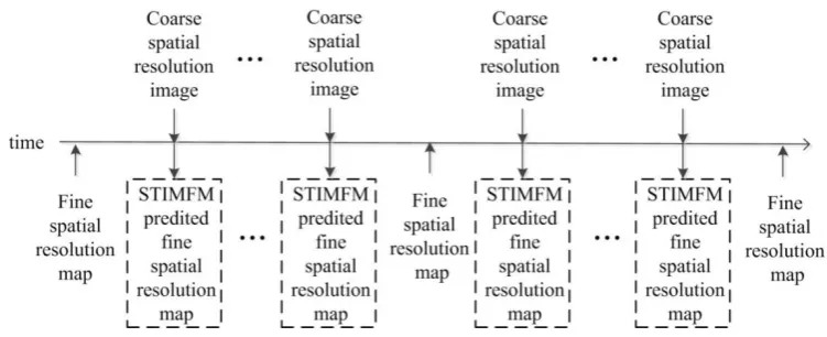
temporal resolution land cover maps. It uses a series of coarse spatial resolution 244

remotely sensed images and a few fine spatial resolution land cover maps as input (Fig. 245

1). STIMFM comprises several main steps, including spectral endmember estimation, 246

analysis of land cover class fraction temporal change, objective function construction, 247

and model optimization. The STIMFM flowchart is shown in Fig. 2. 248

13

250

Fig. 1 Production of a series of fine spatial and temporal resolution land cover maps from a series of 251

coarse spatial resolution remotely sensed images and a few fine spatial resolution land cover maps in 252

STIMFM. 253

254

255

Fig. 2 Flowchart of STIMFM. 256

14

In STIMFM, endmembers that are representative of the spectra of pure land cover 258

classes are estimated for coarse spatial resolution remotely sensed images. Endmember 259

spectra need to be extracted for each coarse spatial resolution image in the dataset as 260

differences may be expected in a time series due to issues such as phenology or 261

variation in image acquisition properties (e.g., angular viewing geometry). Although 262

many endmember extraction algorithms are available, they are not directly used in 263

STIMFM because spectral endmembers are difficult to extract accurately from coarse 264

spatial resolution remotely sensed images due to the small proportion of pure pixels 265

that are typically contained. Information for the estimation of endmembers is instead 266

provided by the fine spatial resolution land cover maps that pre- and post-date the 267

coarse spatial resolution image time series. 268

The land cover classes are defined in the fine spatial resolution land cover maps. 269

For each coarse spatial resolution remotely sensed image, the linear mixture model 270

(LMM) is applied in STIMFM to estimate endmember spectra. With the LMM, the 271

spectral response of each coarse spatial resolution pixel is viewed as being composed 272

of a weighted linear sum of the endmember spectra within that pixel, in which the 273

weights are determined by the relative areal proportions of each endmember (Settle and 274

Drake 1993). On the basis of the linear mixing assumption, the spectral signature yij for

275

the coarse spatial resolution pixel (i,j) in Y can be represented by 276

i ij E j

y f (1) 277

where yij is a B × 1 spectral vector. B is the number of spectral bands. E is a B × C

278

matrix that represents the endmembers used for Y. fij is the C × 1 vector that represents

15

fractions of all endmembers in the pixel (i,j) in Y. 280

Theoretically, to solve for E with B × C unknown variables, at least B × C 281

equations are required. l (l>C) coarse pixels are collected to compose a system of linear 282

mixture equations 283









(2) 284

where yl is the spectral signature for the l-th coarse spatial resolution pixel in Y, and fl

285

is the fraction vector of different classes in the l-th coarse spatial resolution pixel in Y.

286

E can be solved on the basis of the inversion of Eq. (2) by computing a least squares

287

best fit solution 288

2 1

[ ] arg min

l

n n n

f



 

 _  _





E y  (3)

289

where yn is the n-th coarse spatial resolution pixel's spectral signature in Y, and fn is the

290

fraction vector in the n-th coarse spatial resolution pixel in Y. 2 is the L2 norm of

291

the residual vector. "argmin" means the minimizing argument of the function. 292

A number of coarse spatial resolution pixels in Y with known endmember fractions

293

are sought to solve Eq. (3). For each class, the focus is a set of coarse-resolution pixels 294

that have the least changed fractions of that class during the time period covered by Xpre

295

and Xpost. To avoid the collinearity problem in the use of LMM (van der Meer and Jia

296

2012), m coarse-resolution pixels that have the highest fraction of a given class (i.e.,

297

the m purest resolution pixels of the class) among the selected set of

coarse-298

resolution pixels are used. All the m × C coarse spatial resolution pixels are used for

299

endmember estimation in Eq. (3), which can be solved by computing a least squares 300

best fit solution. Assuming the fractions of the m × C coarse spatial resolution pixels

16

are unchanged, the fractions of these coarse pixels in Xpre or Xpost are used as a substitute

302

of those in Y. The fractions in Xpre and Xpost are produced through a spatial degradation

303

process by dividing the number of fine spatial resolution pixels of each class by the 304

total number of fine spatial resolution pixels in a coarse spatial resolution pixel (i.e., s2). 305

2.3. Analysis of land cover class fraction temporal change 306

With the estimated endmembers, class fraction images that represent the area 307

percentage of a pixel occupied by each endmember can be extracted from coarse spatial 308

resolution image Y using the estimated endmember spectra E and on the basis of the

309

mean square error minimization criterion of the LMM 310

2

[f_ij]arg min y_ij f_ij (4) 311

0 f_ijc1, c1, ,C (5) 312

1

1

C ijc c

f







where f_ij  f_ij1,f_ij2, ,f_ijC_T, and fijc is the fraction value of the c-th endmember in

314

coarse spatial resolution pixel (i,j) in Y. 315

The fraction images produced from the coarse spatial resolution image by spectral 316

unmixing, as well as those produced by spatially degrading the fine spatial resolution 317

land cover maps that pre- and post-date the coarse spatial resolution image, provide the 318

land cover trajectory at the acquisition times of Xpre, Y, and Xpost. The change of class

319

fractions in each coarse spatial resolution pixel represents the temporal transitions 320

between classes in the period between the dates of image acquisition. If the class 321

17

map that pre- or post-dates it, then the fine spatial resolution pixel class labels may 323

probably also be unchanged during this period. In this case, the images are temporally 324

correlated. By contrast, if the class fractions changed drastically between two images, 325

then the fine spatial resolution pixels may have changed during this period. Thereby, 326

the images are temporally uncorrelated. As a result, the temporal dependence between 327

different images can be analyzed on the basis of the change in fractions in each coarse 328

spatial resolution pixel. 329

Assume aijk is the k-th (k1, ,s2) fine spatial resolution pixel in the coarse

330

spatial resolution pixel (i,j) (i1, ,I , j1, ,J) in the land cover map X, aijk,pre

331

and aijk,post are the k-th fine spatial resolution pixel in coarse spatial resolution pixel (i,j)

332

in the maps Xpre and Xpost, and c(aijk), c(aijk,pre), and c(aijk,post) are land cover class labels

333

for fine spatial resolution pixels aijk, aijk,pre, and aijk,post, respectively. The temporal

334

dependence or correlation between fine spatial resolution pixels aijk,pre and aijk during

335

Xpre and Y observation period or between fine spatial resolution pixels aijk and aijk,post

336

during Y and Xpost observation period, which is dependent on the class labels of aijk,pre

337

and aijk or the class labels of aijk and aijk,post [Eqs. (7)–(8)] and the change in fractions in

338

this coarse pixel measured by wij,pre and wij,post [Eqs. (9)–(10)], can be characterized as

339

, ( ( ), ( , ))

ij pre ijk ijk pre

w  c a c a or wij post, (c a( ijk), (c aijk post, )).

340

  



,

if

( ), ( 1

( )

0 otherwis )

e

ijk ijk pre ijk ijk pre

c a c a

c a c a

 _ 

 (7)

341

 

if ( )

( ), (

wise )

er

ijk ijk post ijk ijk post

c a c a

c a c a

 _ 

 _. (8)

342

18

spatial resolution pixel in different images have an unchanged class label, thereby 344

indicating that different image pixels are temporally correlated, and a value of 0 if the 345

fine spatial resolution pixel in different images have changed class labels, thereby 346

indicating that the different image pixels are temporally uncorrelated. 347

The changes in fractions in coarse-resolution pixel (i,j) during Xpre and Y

348

observation period and during Y and Xpost observation period are measured by wij,pre

349

and wij,post on the basis of the Gaussian model in Eqs. (9)–(10)

350





, exp ,

ij pre ij ij pre

w =  f  f

(9) 351





, exp ,

ij post ij ij post

w =  f  f

(10) 352

where fij,pre and fij,post are the land cover fraction vector in coarse pixel (i,j) in Xpre and

353

Xpost produced by spatially degrading Xpre and Xpost according to the scale factor s. wij,pre

354

and wij,post indicate the strength of temporal dependence between fine pixels in coarse

355

pixel (i,j) during Xpre and Y observation period or during Y and Xpost observation period.

356

wij,pre and wij,post decrease with the increase in the change of fractions in Eqs. (9)–(10).

357

2.4. Spatial–temporal SRM model 358

Given the coarse spatial resolution image Y, the fine spatial resolution maps Xpre

359

and Xpost, STIMFM aims to predict the fine spatial resolution land cover map X at the

360

time of Y observation. The optimal STIMFM result X, given Y, Xpre ,and Xpost, can be

361

formulated by applying the maximum a posteriori rule in Bayesian framework, i.e., by 362

19













arg max , ,

1

arg max exp , ,

posterior pre post posterior pre post P U Z   _{ }  _{ } _  

X X Y X X

X Y X X

(11) 364

where Z is a normalizing constant. Pposterior





probability of X, given Y, Xpre,and Xpost. Uposterior





366

energy function of X, given Y, Xpre , and Xpost. The solving of (11) is complicated

367

because it involves the optimization of a global distribution model of the entire image. 368

Based on the Markov random field approach, the searching of the optimal X is

369

equivalent to minimization the posterior energy function, which can be specified to 370

model the spatial and temporal dependencies of pixel on its spatial and temporal 371

neighborhoods (Cai et al. 2014; Li et al. 2014). 372





posterior

pre

l spati

post pre p

al temporal

ost

U U U

U X Y X X Y X  X  X X X (12) 373

where Uspectral(Y X) is spectral constraint function that represents the inconsistency

374

between Y and X, Uspatial( )X and Utemporal(X X_pre,X_post) are the spatial and temporal 375

constraint functions, respectively. 376

2.4.1 Spectral constraint function 377

The spectral constraint function is used to link the fine spatial resolution land cover 378

map X with the observed coarse spatial resolution image Y. The spectral response of a

379

coarse spatial resolution pixel in Y is composed of a weighted linear sum of endmember

380

spectral responses within that pixel in the fine spatial resolution map X on the basis of

381

the LMM. A synthetic coarse spatial resolution pixel spectral signature is developed for 382

a coarse spatial resolution pixel on the basis of the endmember spectral signatures and 383

20

constraint function aims to minimize the L2 norm of the residual vector between the 385

observed and synthetic coarse spatial resolution spectral signatures 386

2

1 1

( ) _ij

I J spectral ij i j U f   



Y X y  (13)

387

where the class fraction vector f_ij is calculated by dividing the number of

fine-388

resolution pixels of different classes in coarse-resolution pixel (i,j) by s2 in X, which is 389

estimated and iteratively updated from STIMFM. f_ij is the synthetic spectra for

390

coarse-resolution pixel (i,j) on the basis of the LMM.

391

2.4.2 Spatial constraint function 392

The spatial constraint function is used to describe the spatial pattern of land cover 393

distribution. In STIMFM, the maximal spatial dependence model that aims to maximize 394

the spatial dependence between neighboring fine spatial resolution pixels was used for 395

its simplicity and effectiveness (Atkinson 2009). For a fine spatial resolution pixel a_ijk,

396

the spatial dependence is quantified with respect to its neighboring fine spatial 397

resolution pixels. The STIMFM spatial constraint function is computed as 398



 



2

1 1 1 ( )

1

( )= ( ), ( )

,

ijk

I J s spatial

s ijk l

i j k l a _{ijk l}

U c a c a

d a a

               





where N(aijk) is the spatial neighborhood that includes all fine spatial resolution pixels

400

inside a square window whose center is aijk (aijk itself is not included), and al is a

401

neighboring fine spatial resolution pixel of aijk in N(aijk). The size of the neighborhood

402

N(aijk) is W. d a





403

cover class label for fine spatial resolution pixel al. 





404

and c(al) are the same and 0 otherwise. _S is the spatial weight parameter. -_S is

21

multiplied because the STIMFM objective function seeks the minimal value as the 406

optimal solution. 407

2.4.3 Temporal constraint function 408

The STIMFM temporal constraint function is used to measure the temporal 409

dependence between the predicted fine spatial resolution map X and the input fine

410

spatial resolution maps Xpre and Xpost. The class label of fine spatial resolution pixel aijk

411

is temporally correlated to fine spatial resolution pixel aijk,pre and aijk,post in the maps Xpre

412

and Xpost depending on the class labels of aijk, aijk,pre and aijk,post and the strength of

413

temporal dependences measured by the weights wij,pre and wij,post. _T is the temporal

414

weight parameter. The STIMFM temporal constraint function is written as 415

















2

, ,

, ,

1 1 1

( _pre, _post)= _{ij pre} ( ), ( _pre) _i ( ), ( )

I J s

j pos temporal

T ijk ijk ijk ijk post i k

t j

U  w  c a c a w  c a c a

  

    



X X X (15)

416

2.5. Model initialization and optimization 417

An initial fine spatial resolution land cover map is used as input to STIMFM at the 418

outset. The initialization map is produced according to the land cover class fraction 419

images estimated from a coarse spatial resolution image. The fine spatial resolution 420

pixels are randomly allocated class labels in a manner that maintains the class 421

proportional information conveyed by a prior spectral unmixing analysis (Kasetkasem 422

et al. 2005). The class labels in the initial fine spatial resolution land cover map are then 423

updated iteratively. Here, the Iterative Conditional Mode (ICM) was applied to 424

22

labels change during two successive iterations or when a predefined number of 426

iterations have been undertaken. 427

3. Experiments and results

The proposed STIMFM was evaluated in three experiments. The first used Landsat 429

multi-spectral images and the National Land Cover Database (NLCD) land cover maps 430

(Landsat–NLCD). The second used MODIS and Landsat multi-spectral images 431

(MODIS–Landsat). The third used Landsat and Google Earth Images (Landsat–GEI). 432

For a rigorous assessment, several traditional approaches were used for comparison, 433

including the Pixel Swapping based SRM (PS_SRM) (Atkinson 2005), the Spatial 434

Regularization based SRM (SR_SRM) (Ling et al. 2014), the ESTARFM (Zhu et al. 435

2010), and the FSDAF model (Zhu et al. 2016). 436

PS_SRM and SR_SRM use only a mono-temporal coarse spatial resolution image 437

as input and hence do not exploit the temporal information in the land cover. By contrast, 438

ESTARFM uses a coarse spatial resolution image and pairs of coarse and fine spatial 439

resolution images that pre-and post-date it as input. ESTARFM is based on the 440

assumption that remotely sensed data from different satellite sensors observed on the 441

same, or at least very close, date are mutually comparable and correlated, and uses the 442

correlation to blend multi-source data and minimize the system biases. The FSDAF, 443

which is based on spectral unmixing analysis and a thin plate spline interpolator, is also 444

used for comparison. It requires only one pair of fine and coarse spatial resolution 445

images that pre- or post-date the coarse-resolution image. 446

23

than a land cover map. The fine spatial resolution image produced may then be 448

classified. Two types of classification methods were applied. The first one is the 449

Maximum Likelihood Classifier (MLC), which is one of the statistical classifiers that 450

relies on the second-order statistics of a Gaussian probability density function for the 451

distribution of the feature vector of each class. In MLC, a pixel is allocated to the class 452

with which it has the highest likelihood of membership (Richards and Jia 1999). The 453

produced final fine spatial resolution land cover maps by MLC, which are referred to 454

as ESTARFM_MLC and FSDAF_MLC, were compared with STIMFM. 455

The second used classification method is the automated Land Cover updating 456

approach based on integrated change detection and classification methods (LCupdating) 457

produced by Chen et al. (2012). MLC used only the fused fine-resolution image as input 458

but ignored the available fine-resolution image and land cover map that pre- or post-459

dates the coarse-resolution image. LCupdating was applied to the fused image from 460

ESTARFM and FSDAF by incorporating the fine-resolution remotely sensed image and 461

land cover map that pre-date the coarse-resolution image. LCupdating first detects 462

changes between the input and fused fine-resolution images from ESTARFM or 463

FSDAF and then predicts the changed pixel labels in the fused image based on the 464

Markov random field based classifier. The ESTARFM and FSDAF incorporating 465

LCupdating methods (ESTARFM_LCupdating and FSDAF_LCupdating) were 466

compared with STIMFM. 467

The parameters of these different methods were set according to results reported 468

in the literature and through trial and error. The STIMFM spatial weight parameter S

24

and temporal weight parameter _T were set to 0.05. The neighborhood window size

470

W in the STIMFM spatial constraint function was set to 2×s-1 (Tolpekin and Stein

471

2009). The number of unchanged coarse pixels, m, in STIMFM endmember estimation

472

was set to 100. 473

474

3.1 Landsat–NLCD experiment 475

3.1.1 Data preparation 476

This experiment used Landsat Thematic Mapper (TM) multi-spectral images and 477

NLCD land cover maps. The NLCD is a land cover classification scheme of Albers 478

Equal Area projection, which has been applied consistently at a spatial resolution of 479

30 m across the conterminous USA primarily on the basis of Landsat satellite data. 480

NLCD maps for the years 2001, 2006, and 2011 were used in this experiment. The 481

NLCD 2001 was based primarily on a decision tree classification of 2001 Landsat 482

satellite data. The NLCD 2006 and 2011 were based primarily on a decision tree 483

classification from 2006 and 2011 Landsat satellite data, and also quantified land cover 484

change from 2001 to 2006 and 2006 to 2011 (Homer et al. 2015; Jin et al. 2013; Xian 485

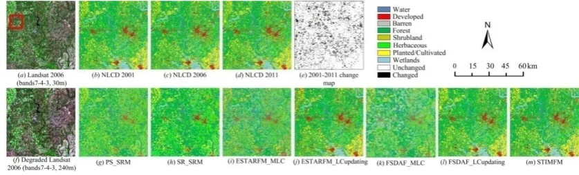
et al. 2009). The original sixteen classes were reclassified into eight classes (Fig. 3). 486

Subset land cover maps, each with a size of 2000 × 2000 pixels (centered at 34°4′00″N

487

and 79°27′00″W), were acquired from NLCD 2001, 2006, and 2011 [Fig. 3(b–d)].

488

25

490

Fig. 3 Input and result maps for the entire study area in the Landsat–NLCD experiment. 491

492

A Landsat TM image (path 016, row 036) acquired on April 9, 2006 in the study 493

area was downloaded from the United States Geological Survey (USGS). This Landsat 494

image was re-projected to the Albers Equal Area projection, and six spectral bands at 495

the spatial resolution of 30 m (the 120 m thermal infrared band was excluded) were 496

used to extract the same 2000 × 2000 pixel area that was identified in the NLCD maps 497

[Fig. 3(a)]. The subset image was calibrated to surface reflectance (Gao et al. 2006;

498

Masek et al. 2006) and then spatially degraded to simulate a coarse spatial resolution 499

multi-spectral image using a scale factor s=8 [Fig. 3(f), 240 m] with a mean filter. The

500

NLCD 2006 [Fig. 3(c)] was used as the reference map used for accuracy assessment.

501

The pixels that changed land cover class from 2001 to 2011 accounted for 12.08% of 502

all fine spatial resolution pixels. 503

For analyses with the PS_SRM and SR_SRM, only the degraded multi-spectral 504

image [Fig. 3(f)] was needed as input. For the STIMFM, the required input included

505

the degraded multi-spectral image [Fig. 3(f)] and the NLCD 2001 and NLCD 2011 land

506

cover maps [Fig. 3(b), 3(d)]. For ESTARFM, pairs of fine and coarse spatial resolution

507

26

remotely sensed image were needed. To obtain the required data, a Landsat TM image 509

acquired on April 17, 2001 and a Landsat TM image acquired on April 7, 2011 were 510

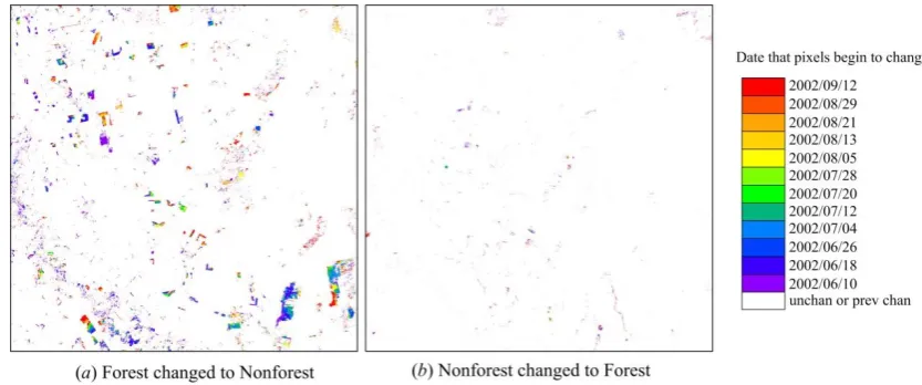
also downloaded, re-projected, subsetted, and calibrated. The original 30 m spatial 511

resolution reflectance images with six spectral bands (the 120 m thermal infrared band 512

was excluded) were spatially degraded to simulate their corresponding coarse spatial 513

resolution multi-spectral images at scale factors s=8, respectively. Therefore, the input

514

to the ESTARFM_MLC and ESTARFM_LCupdating included fine and coarse spatial 515

resolution multi-spectral image pairs in 2001 and 2011 and the coarse spatial resolution 516

multi-spectral image for 2006. The input to FSDAF_MLC and FSDAF_LCupdating 517

included fine and coarse spatial resolution multi-spectral image pairs in 2001 and the 518

coarse spatial resolution multi-spectral image in 2006. In ESTARFM_LCupdating and 519

FSDAF_LCupdating, the NLCD 2001 fine-resolution land cover map was also used as 520

the base data. 521

522

3.1.2 Results 523

524

27

The land cover maps produced from the different methods are shown in Fig. 3 for 526

the entire area and in Fig. 4 for the zoomed area [320 × 320 pixel area in Fig. 3(a)]. In

527

the zoomed area, the PS_SRM map contained many speckle-like artifacts [Fig. 4(g)].

528

This situation arises because the spectral unmixing may determine a small fractional 529

cover of a class that is actually absent in a coarse-resolution pixel, and this fraction 530

must be maintained in the result. The SR_SRM map contained fewer speckle-like 531

artifacts than PS_SRM, because SR_SRM relaxed the constraint of land cover fraction 532

maintenance [Fig. 4(h)]. However, the maximal spatial dependence model used in

533

SR_SRM also led to rounded land cover patches. Compared with PS_SRM and 534

SR_SRM, more spatial detail of the land cover mosaic was retained in the ESTARFM, 535

FSDAF, and STIMFM maps. Many speckle-like artifacts in the ESTARFM_MLC [Fig. 536

4(i)] and FSDAF_MLC [Fig. 4(k)] maps existed because MLC is a per-based

537

classification method, and the spatial context information was not used. 538

ESTARFM_MLC and FSDAF_MLC incorrectly classified cases that have similar 539

reflectance values, such as “forest”, “herbaceous”, and “wetlands”, in the result maps 540

[Figs. 4(i), (k)]. 541

542

Fig. 5 Landsat, ESTARFM and FSDAF images in the zoomed area for the Landsat–NLCD experiment. 543

In contrast to ESTARFM_MLC and FSDAF_MLC, ESTARFM_LCupdating [Fig. 544

4(j)] and FSDAF_LCupdating [Fig. 4(l)] quantified the land cover changes between

545

28

map [Fig. 4(c)]. The labels of pixels that were detected as unchanged by LCupdating

547

were preserved in the ESTARFM_LCupdating and FSDAF_LCupdating maps. The 548

labels of changed pixels were determined based on the Markov random field based 549

classifier, which considers the contextual information in classification. Thus, most 550

speckle-like artifacts were eliminated in ESTARFM_LCupdating and

551

FSDAF_LCupdating. However, many changed pixel labels were incorrectly predicted 552

by ESTARFM_LCupdating and FSDAF_LCupdating. “Herbaceous” was incorrectly 553

labeled as “developed” in the ESTARFM_LCupdating highlighted by the black circle 554

[Fig. 4(j)], and the linear-shaped “developed” in the FSDAF_LCupdating highlighted

555

by the black circle was disconnected [Fig. 4(l)]. The predicted reflectance for pixels of

556

changed land cover for “herbaceous” and “planted/cultivated” in ESTARFM [e.g., 557

those highlighted by the red circle in Fig. 5(f)] was dissimilar to that in the Landsat

558

2006 reference image [Fig. 5(b)] because ESTARFM cannot capture abrupt land cover

559

changes (Zhu et al. 2010), and the predicted reflectance of linear-shaped “developed” 560

land cover was similar to that of “planted/cultivated” in the FSDAF image highlighted 561

by the red circle in Fig. 5(g), because FSDAF cannot capture tiny land cover changes

562

(Zhu et al. 2016). By contrast, the STIMFM land cover map as shown in Fig. 4(m) was

563

quite similar to the reference map, and the detailed land cover patterns were well 564

represented. STIMFM correctly predicted the class labels not only for almost all pixels 565

of unchanged land cover but also for most of those pixels for which land cover class 566

had changed, such as those highlighted in the red circle in Fig. 5(d).

567

29 Table 1

569

Overall accuracies (OAs) and accuracies of different methods in predicting PULC and PCLC in the 570

Landsat–NLCD experiment. 571

OA PULC PCLC

PS_SRM 41.61 41.54 42.13

SR_SRM 49.10 49.01 49.77

ESTARFM_MLC 33.57 35.10 22.44

ESTARFM_LCupdating 88.28 94.89 40.18

FSDAF_MLC 33.60 34.29 28.60

FSDAF_LCupdating 89.50 96.15 41.08

STIMFM 94.89 99.24 63.27

572

The overall accuracies of different methods are shown in Table 1. The result maps 573

were compared with the NLCD 2006. The overall accuracy of STIMFM is higher than 574

those obtained from the other methods. Table 1 also shows the accuracies of pixels of 575

changed and unchanged land cover (PULC means the percentage of correctly labeled 576

pixels of unchanged land cover among all pixels of unchanged land cover, and PCLC 577

means the percentage of correctly labeled pixels of changed land cover among all pixels 578

of changed land cover) obtained from the different methods. For PS_SRM and 579

SR_SRM, which applied a mono-temporal remotely sensed image, no obvious 580

difference was found between PULC and PCLC values. For ESTARFM, FSDAF, and 581

STIMFM applied to multi-temporal data, the PULC values were higher than the PCLC 582

values. These results indicate that extracting changed land cover information is more 583

difficult than extracting unchanged land cover information from ESTARFM, FSDAF, 584

and STIMFM. STIMFM integrates the temporal dependence model in its objective 585

30

those in the pre- and post-dated fine-resolution land cover maps. If the fine-resolution 587

pixel class labels are unchanged during the observation period, then STIMFM could 588

make the best use of pixel class labels in the fine-resolution maps that pre- and post-589

date the coarse-resolution image. Thus, the accuracies for classes with unchanged class 590

labels are high. By contrast, if the fine-resolution pixel class labels have changed during 591

the observation period, then STIMFM could not make the best use of pixel class labels 592

in the fine-resolution maps that pre- and post-date the coarse-resolution image, and the 593

accuracies for classes with changed class labels are relatively low. The PULC was 594

higher than 99%, and the PCLC was higher than 63% for STIMFM; these values are 595

higher than those obtained from the other methods. 596

597

3.2 MODIS–Landsat experiment 598

3.2.1 Data preparation 599

The study area was located near Sorriso (12°33′00″S and 55°42′00″W) in Mato 600

Grosso State, Brazil. This area was mainly covered by tropical forests but has suffered 601

from deforestation in recent years (Hansen et al. 2008). This experiment used eleven 602

coarse spatial resolution MODIS images and two fine spatial resolution land cover 603

maps that pre- and post-date the coarse spatial resolution image series as input and 604

outputs eleven fine-resolution land cover maps with MODIS repetition rates to show 605

the fine spatial and temporal deforestation process in the study area. Landsat Enhanced 606

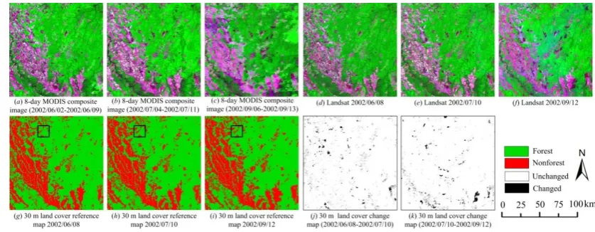
Thematic Mapper Plus (ETM+) images (path 226, row 069) acquired on 2002/06/08 607

and 2002/09/12 were downloaded from USGS [Fig. 6(d) and (f)]. Data in six bands (the

31

120 m thermal infrared band was excluded) at the 30 m spatial resolution with the 609

Universal Transverse Mercator projection were used and calibrated to surface 610

reflectance values (Gao et al. 2006; Masek et al. 2006). One cloud-free Landsat ETM+ 611

image acquired on 2002/07/10 was used for accuracy assessment [Fig. 6(e)]. A total of

612

thirteen eight-day surface reflectance MODIS product (MOD09A1) datasets that 613

comprise seven spectral bands (620 nm–2055 nm) with a spatial resolution of 463 m 614

acquired from 2002/06/02 to 2002/09/13 were downloaded from USGS (Walker et al. 615

2012). The MODIS images were re-projected into the UTM coordinate system and 616

resampled to a spatial resolution of 450 m using the nearest neighbor interpolation, and 617

were adopted as the coarse spatial resolution multi-spectral images required for the 618

analyses. The study area covers 300 × 300 MODIS pixels, which correspond to 4500 × 619

4500 Landsat pixels, with a scale factor s=15.

620

621

622

Fig. 6 MODIS, Landsat images, and reference maps in the MODIS–Landsat experiment from 623

2002/06/08 to 2002/09/12. 624

625

32

spatial resolution [Fig. 6(g)–(i)]. Two land cover classes, forest and nonforest, were 627

considered in this experiment. The endmembers of each class were manually selected 628

from each Landsat image, and MLC was applied to generate the fine spatial resolution 629

forest/nonforest reference maps. The fine-resolution change maps that produced by a 630

per-pixel comparison of maps in Fig. 6(g)–(i) are shown in Fig. 6(j)–(k). The pixels that

631

changed land cover class from 2002/06/08 to 2002/09/12 accounted for 4.30% of all 632

fine spatial resolution pixels. 633

STIMFM used the MODIS multi-spectral image series from 2002/06/10 to 634

2002/09/05 and the 2002/06/08 and 2002/09/12 fine spatial resolution land cover maps 635

in Fig. 6 (g) and (i) as input and predicted a series of land cover maps at 30 m spatial

636

resolution with MODIS repetition rates during this period. The accuracy was assessed 637

using the 2002/07/10 land cover map [Fig. 6(h)]. The STIMFM was compared with

638

PS_SRM, SR_SRM, ESTARFM_MLC, ESTARFM_LCupdating, FSDAF_MLC, and 639

FSDAF_LCupdating using the 2002/07/10 land cover map in Fig. 6(h) for assessment.

640

In these methods, the eight-day composite MODIS image [2002/07/04–2002/07/11 in 641

Fig. 6(b)] was used as the coarse-resolution image. Aside from this data, ESTARFM

642

used the eight-day composite MODIS images [2002/06/02–2002/06/09 in Fig. 6(a) and

643

2002/09/06–2002/09/13 in Fig. 6(c)] and Landsat multi-spectral images [2002/06/08 in

644

Fig. 6(d) and 2002/09/12 in Fig. 6(f)] as input, and FSDAF used the eight-day

645

composite MODIS image [2002/06/02–2002/06/09 in Fig. 6(a)] and Landsat

multi-646

spectral image [2002/06/08 in Fig. 6(d)] as input. In ESTARFM and FSDAF, the

647

33

spectral band of Landsat image was observed from MODIS band 5. The 2002/06/08 649

fine spatial resolution land cover map in Fig. 6(g) was also inputted in the

650

ESTARFM_LCupdating and FSDAF_LCupdating. 651

3.2.2 Results 652

653

34 Table 2

655

Overall accuracies (OAs) and accuracies of different methods in predicting PULC and PCLC in the 656

MODIS–Landsat experiment. The MODIS image used in different methods was the eight-day composite 657

data from 2002/07/04 to 2002/07/11. 658

OA PULC PCLC

PS_SRM 88.14 89.29 62.52

SR_SRM 89.28 _{90.42 63.73}

ESTARFM_MLC 95.17 _{96.90 56.71}

ESTARFM_LCupdating 96.32 98.07 57.42

FSDAF_MLC 95.07 96.72 58.23

FSDAF_LCupdating 96.61 98.37 57.38

STIMFM 98.27 99.69 66.67

659

The OA, PULC, and PCLC values obtained from the application of the different 660

methods are shown in Table 2. The overall accuracies obtained from the PS_SRM and 661

SR_SRM were lower than 90%, whereas the overall accuracies of ESTARFM_MLC, 662

ESTARFM_LCupdating, FSDAF_MLC, and FSDAF_LCupdating were higher than 663

95%. These findings indicate that the classification from fine-resolution image 664

extracted by spatial–temporal fusing of coarse and fine-resolution images can better 665

improve the accuracy compared with SRM applied to a mono-temporal coarse-666

resolution image. The OA value for STIMFM was 98.27%, which is higher than all the 667

other methods. The PCLC values were lower than the PULC values for ESTARFM, 668

FSDAF, and STIMFM methods, which is similar to those in the Landsat–NLCD 669

experiment. The STIMFM has the highest PULC value, which was 99.69%, and the 670

35

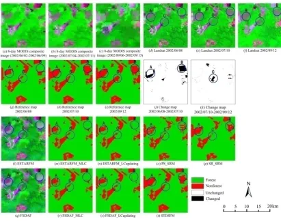
672

Fig. 7 Input, reference, and result images and maps for the zoomed area at different years for the MODIS– 673

Landsat experiment. The MODIS image used in different methods was the eight-day composite data 674

from 2002/07/04 to 2002/07/11. 675

676

The reference, input, and result images and maps in the zoomed area are shown in 677

Fig. 7. A part of the forest patch (highlighted by a blue circle in regions A and B in Fig. 678

7) changed to nonforest from 2002/06/08 to 2012/07/10 [Fig. 7(j)], and a part of the

679

forest patch (highlighted by a blue circle in region C in Fig. 7) changed to nonforest 680

from 2002/07/10 to 2012/09/12 [Fig. 7(k)]. The PS_SRM map contained many

speckle-681

like artifacts [Fig. 7(o)], and SR_SRM contained land cover patches with oversmoothed

682

rounded boundaries [Fig. 7(p)]. In the ESTARFM and FSDAF fused images [Fig. 7(l),

683

(q)], the pixels of unchanged land cover considerably resemble those in the reference

36

Landsat image, whereas the pixels of changed land cover (highlighted by blue circles 685

in Fig. 7) were noticeably different from those in the reference Landsat image [Fig. 686

7(e)]. As a result, these pixels of changed land cover were erroneously classified in the

687

ESTARFM_MLC, ESTARFM_LCupdating, FSDAF_MLC, and FSDAF_LCupdating 688

results [Figs. 7(m), (n), (r), and (s)]. By contrast, most of the changed and unchanged

689

pixels are correctly allocated by STIMFM [Fig. 7(t)], thereby showing the ability of the

690

proposed STIMFM model in the reconstruction of land cover trajectories for pixels of 691

both changed and unchanged land cover. The land cover changes in Fig. 8 were 692

extracted by comparing the STIMFM predicted maps and input fine-resolution land 693

cover map that pre-dates the coarse images [Fig. 6(g)]. The colors in Fig. 8 indicate the

694

date when the pixels begin to change. The forest area decreased gradually, whereas the 695

nonforest area increased in Fig. 9. With STIMFM, the detailed spatial extent 696

information and the change of areas for different classes can be extracted, thereby 697

showing the effectiveness of the proposed method. 698

37

700

Fig. 8 30 m spatial extent of land cover change with MODIS repetition rates derived from STIMFM. The 701

colors represent the date when pixels begin to change. “unchan or prev chan” marked as white color 702

means unchanged or previously changed before 2002/06/08. 703

704

705

Fig. 9 Forest and nonforest areas extracted using STIMFM in the MODIS–Landsat experiment. 706

707

708

3.3 Landsat–GEI experiment 709

The study area was located in Wuhan (30°27′30″N and 114°32′30″E), Hubei

710

province, China. This area underwent rapid urbanization in 2010–2016. This 711

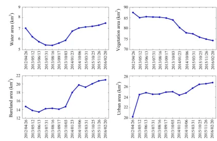
experiment used eleven cloud-free 30 m spatial resolution Landsat-8 Operational Land 712

38

5 m spatial resolution land cover maps acquired in 2012 and 2016 as input. Eleven 5 m 714

resolution land cover maps during 2013–2015 were predicted to show the fine spatial 715

and temporal urbanization process in the study area. The acquired eleven Landsat OLI 716

images were downloaded from USGS. The first seven bands of OLI image with a spatial 717

resolution of 30 m were selected. Two GEIs acquired on 2012/04/26 and on 2016/02/20 718

[Figs. 10(a), (b)] with a spatial resolution of 5 m were re-projected into the UTM 719

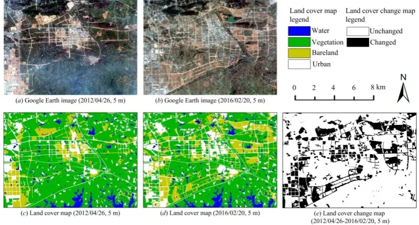
coordinate system and digitized into the 5 m land cover maps [Figs. 10(c), (d)]. Four

720

land cover classes, namely, water, vegetation, bareland, and urban, were found in the 721

fine-resolution maps. The study area covers 320 × 450 Landsat pixels, which 722

correspond to 1920 × 2700 fine-resolution pixels in Figs. 10(c) and (d), with a scale

723

factor s = 6. The land cover change map from 2012/04/26 to 2016/02/20 is shown in

724

Fig. 10(e). The pixels that changed land cover class accounted for 23.49% of all fine

725

spatial resolution pixels from 2012/04/26 to 2016/02/20. 726

39

728

Fig. 10 Google Earth images, land cover maps and change maps in the Landsat–GEI experiment. 729

730

STIMFM was used to produce the eleven 5 m resolution land cover maps with 731

Landsat repetition rates during 2013–2015 using the eleven cloud-free Landsat images 732

and two 5 m land cover maps on 2012/04/26 and 2016/02/20 as input. The STIMFM 733

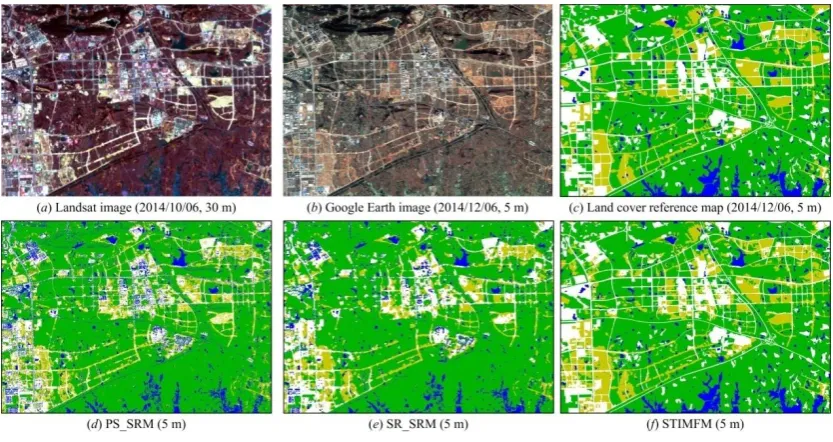
accuracy was assessed using a 5 m fine-resolution land cover map, which was produced 734

according to a GEI at the spatial resolution of 5 m acquired on 2014/12/06 [Fig. 11(b)].

735

This GEI is the only fine-resolution one available in the study area during 2012–2016 736

and was re-projected into the UTM coordinate system and digitized to the reference 737

land cover map [Fig. 11(c)]. STIMFM was compared with PS_SRM and SR_SRM,

738

which were applied to a single-date Landsat OLI image acquired on 2014/10/06 [Fig. 739

11(a)]; this image is temporally closest to the GEI in 2014 [Fig. 11(b)]. ESTARFM and

740

FSDAF were not used for comparison because they require the coarse- and fine-741

resolution images to have comparable and correlated reflectance bands, whereas 742

40

into reflectance images, which are correlated to the Landsat images. 744

745

Table 3

746

Overall accuracies (OAs) and accuracies of different methods in predicting PULC and PCLC in the 747

Landsat–GEI experiment. The Landsat image used for assessment in the different methods was acquired 748

on 2014/10/06. 749

OA PULC PCLC

PS_SRM 72.71 76.22 61.13

SR_SRM 73.73 77.29 61.99

STIMFM 94.31 99.61 76.81

750

The OA accuracies were lower than 74% for PS_SRM and SR_SRM and increased 751

to 94.31% for STIMFM (Table 3). The PULC value was higher than 99%, and the 752

PCLC value was higher than 76% for STIMFM; these values were obviously higher 753

than those for PS_SRM and SR_SRM. The PULC values were higher than the PCLC 754

values for STIMFM because STIMFM could make the best use of unchanged pixel 755

labels in the fine-resolution maps that pre- and post-date the Landsat images in land 756

cover mapping. 757