www.atmos-meas-tech.net/9/3607/2016/ doi:10.5194/amt-9-3607-2016
© Author(s) 2016. CC Attribution 3.0 License.
How big is an OMI pixel?
Martin de Graaf1,3, Holger Sihler2, Lieuwe G. Tilstra3, and Piet Stammes3 1Delft University of Technology, Delft, the Netherlands
2Max-Planck-Institut für Chemie, Mainz, Germany
3Royal Netherlands Meteorological Institute, De Bilt, the Netherlands Correspondence to:Martin de Graaf ([email protected])
Received: 29 February 2016 – Published in Atmos. Meas. Tech. Discuss.: 24 March 2016 Revised: 30 June 2016 – Accepted: 7 July 2016 – Published: 4 August 2016
Abstract. The Ozone Monitoring Instrument (OMI) is a push-broom imaging spectrometer, observing solar radiation backscattered by the Earth’s atmosphere and surface. The incoming radiation is detected using a static imaging CCD (charge-coupled device) detector array with no moving parts, as opposed to most of the previous satellite spectrometers, which used a moving mirror to scan the Earth in the across-track direction. The field of view (FoV) of detector pixels is the solid angle from which radiation is observed, aver-aged over the integration time of a measurement. The OMI FoV is not quadrangular, which is common for scanning instruments, but rather super-Gaussian shaped and overlap-ping with the FoV of neighbouring pixels. This has con-sequences for pixel-area-dependent applications, like cloud fraction products, and visualisation.
The shapes and sizes of OMI FoVs were determined pre-flight by theoretical and experimental tests but never veri-fied after launch. In this paper the OMI FoV is characterised using collocated MODerate resolution Imaging Spectrora-diometer (MODIS) reflectance measurements. MODIS mea-surements have a much higher spatial resolution than OMI measurements and spectrally overlap at 469 nm. The OMI FoV was verified by finding the highest correlation between MODIS and OMI reflectances in cloud-free scenes, assuming a 2-D super-Gaussian function with varying size and shape to represent the OMI FoV. Our results show that the OMPIX-COR product 75FoV corner coordinates are accurate as the full width at half maximum (FWHM) of a super-Gaussian FoV model when this function is assumed. The softness of the function edges, modelled by the super-Gaussian expo-nents, is different in both directions and is view angle depen-dent.
The optimal overlap function between OMI and MODIS reflectances is scene dependent and highly dependent on time differences between overpasses, especially with clouds in the scene. For partially clouded scenes, the optimal overlap func-tion was represented by super-Gaussian exponents around 1 or smaller, which indicates that this function is unsuitable to represent the overlap sensitivity function in these cases. This was especially true for scenes before 2008, when the time differences between Aqua and Aura overpasses was about 15 min, instead of 8 min after 2008. During the time between overpasses, clouds change the scene reflectance, reducing the correlation and influencing the shape of the optimal overlap function.
1 Introduction
1.5 nm), from which multiple trace gases, clouds, and aerosol parameters can be retrieved simultaneously. TOMS instru-ments have been monitoring the ozone column at a relatively high spatial resolution (50×50 km2) with daily global cov-erage since 1978. OMI was designed to combine those func-tions and measure the complete spectrum from the UV to the visible wavelength range (up to 500 nm) with a high spatial resolution and daily global coverage. To this end, the imag-ing optics were completely redesigned.
Instead of a rotating mirror, in OMI a two-dimensional CCD (charge-coupled device) detector array (780×576 pixels) is used to map the incoming radiation in the across-track and wavelength dimensions simultaneously. A swath of about 2600 km in the across-track direction is imaged along one dimension of the detector array. Spectrally, the radiation is split into two UV channels and a visible (VIS) channel and imaged along the wavelength dimension of the detector array. The spectral resolution of the VIS channel is 0.63 nm. The along-track direction is scanned due to the movement of the satellite. In default “Global” operation mode, five consecutive CCD images, each with a nominal exposure time of 0.4 s, are electronically co-added during a 2 s interval. The subsatellite point moves about 13 km during this time interval (Levelt, 2002). The consequence of this design is that the spatial response function of the OMI footprints is not box-shaped but has a peak at the centre of the footprint. This new design, avoiding moving parts, was used in OMI for the first time and is now being used in several new, upcoming satellite missions.
The point spread function (PSF) is defined as the response of the imaging system to a point source, while the telescope field of view (FoV) is defined by the projection of the OMI spectrograph slit on the Earth’s surface from the point of view of a CCD pixel. This projection is affected by Fraun-hofer diffraction of the imaging optics, which, for a circu-lar aperture, can be modelled using an Airy function. For a rectangular slit, used in OMI, the solution can be approxi-mated by a Gaussian function in two dimensions. The FoV has been determined pflight by measuring the intensity re-sponse to a star stimulus for all pixels. The rere-sponse func-tion was measured by exposing the pixels to a point source and rotating the instrument. The sensitivity curve found in this way was fitted to a Gaussian curve, of which the full width at half maximum (FWHM) was reported. This is pro-prietary information, but the results are summarised here. In the swath (across-track) direction the average peak position for each pixel was determined and fitted to a linear curve to determine the spatial sampling distance for the three chan-nels, which gives the instantaneous FoVs in the across-track direction for individual pixels. For the VIS channel the FoV for the entire swath is 115.1◦. The PSF in the across-track di-rection was not determined (or reported). However, a memo from the OMI Science Support Team from 2005 shows an across-track pixel size estimation from these measurements, where the sizes have been determined by assuming no
over-lap between adjacent pixels and computing the distances be-tween the peak positions when imaged on the Earth. This yields sizes in the across-track direction of 23.5 km at nadir and 126 km for far off-nadir (56◦) pixels.
In the along-track direction the FoV was characterised by tilting the instrument to simulate the movement in the flight direction. The measurements were fitted to a Gaussian curve with variable width for different across-track angles and wavelengths. This width is reported as the FWHM in de-grees, which is about 0.95 at nadir and 1.60 at 56◦ for the VIS channel. This corresponds to a nadir pixel size in the along-track direction of about 15 km and a far off-nadir pixel size of about 42 km when the Gaussian is convolved with a boxcar function whose width is the 13 km movement of the subsatellite point during the 2 s exposure.
The instantaneous FoV (iFoV) of the OMI instrument is influenced by a polarisation scrambler, which transforms the incoming radiation from one polarisation state into a contin-uum of polarisation states (as opposed to unpolarised light). The incoming beam is split into four beams of equal inten-sity, scrambled, and projected onto the CCD. Since the pro-jections of the four beams are slightly shifted with respect to each other, the polarisation state of the incoming radia-tion still slightly determines the intensity distriburadia-tion of the four beams and therefore the iFoV in the flight direction. The only property which is not dependent on the polarisation state of the incoming radiation is the centre of weight of the four beams. This corresponds to the centre of the ground pixels, which is therefore the only geolocation coordinate that can be determined unambiguously (van den Oord, 2006).
the FoV. The coordinates in the across-track direction, how-ever, are still the half-way points between adjacent pixels.
The application of quadrangular pixel shapes for OMI can become problematic when pixel values are aggregated onto a regular grid (e.g. Level 3 products that are reported on a regular lat.–long. grid). If pixels overlap, which might oc-cur when several orbits are averaged or in the case of 75FoV pixels, extreme values may be smoothed and reduced due to averaging. A more realistic distribution that preserves mean values can be reconstructed using a parabolic spline surface on the quadrangular grid, resulting in a much better visuali-sation (Kuhlmann et al., 2014). In cases where values from OMI are compared with those of another instrument, espe-cially one with a higher spatial resolution, the approximate true shape of an OMI pixel is desired. For example, we intend to combine spectral measurements from OMI and MODIS to determine the aerosol direct effect over clouds (de Graaf et al., 2012). To this end, an optimal characterisation of the FoV of the OMI footprint is desired, to optimise the accuracy of the retrieval.
In this paper, the OMI FoV for the VIS channel is inves-tigated by testing various predefined shapes and sizes under various circumstances and determining the maximal corre-lation between OMI and MODIS reflectances. In Sect. 2, the consistency between overlapping OMI and MODIS re-flectances is investigated. A cloud-free scene from 2008 is used to study the FoV under the most optimal circumstances. In Sect. 3, a two dimensional super-Gaussian function with a varying exponent is introduced, which can change shape from a near-quadrangular to a sharp-peaked distribution. Fur-thermore, the sizes in both along- and across-track directions can be varied. This function is used to define various FoVs, which are investigated for various scenes. The change in FoV is further investigated by looking into the effect of scene and geometry changes during the (varying) overpass times of OMI and MODIS. The conclusions from this study are re-ported in Sect. 4. The geolocations of the pixels in the UV channels are slightly different from those in the VIS channel. However, the FoV cannot be determined in the same way for the UV, since MODIS measurements do not overlap with these channels spectrally.
2 Data
The Aura satellite flies in formation with the Aqua satellite in the afternoon constellation (A-train). Aqua was launched in 2002, to lead Aura in the A-train by about 15 min. The time difference between the instruments within the A-train is con-trolled by keeping the various satellites within control boxes, which are defined as the maximum distances to which the satellites are allowed to drift before correcting manoeuvres are executed. Therefore, the time difference between OMI and MODIS is variable by up to a few minutes. A major orbital manoeuvre in 2008 of Aqua decreased the distance between the Aura and Aqua control boxes to about 8 min.
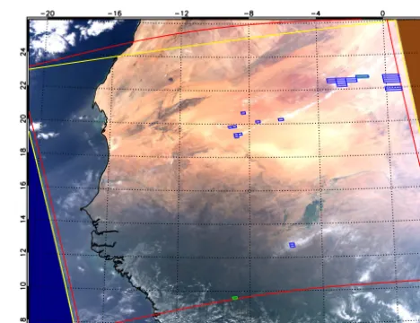
Figure 1.MODIS RGB image of the reference scene on 4 Novem-ber 2008 at 14:00 UTC (start of the central MODIS granule). The yellow lines indicate the MODIS data granules, and the red lines the considered OMI swath, which was confined to rows 2–57, with the exception of pixels in the row anomaly (see text). The green pixels indicate the darkest (vegetated) and the brightest (cloud-covered) areas in the scene. The OMI reflectance spectra of these pixels are shown in Fig. 2. The blue OMI pixels correspond to the blue-marked points in Fig. 3.
To investigate the correlation between OMI and MODIS observed reflectances, several scenes were selected. One ref-erence scene will be discussed here in detail. It was an al-most cloud-free scene over the Sahara on 4 November 2008, around 14:00 UTC (start of the first MODIS granule). At this point in time, the time difference between OMI and MODIS was reduced to 8 min and around 20–30 s, depending on the pixel row. The differences between the pixel times arise from the fact that MODIS has a scanning mirror, while OMI has no scanning optics but exposes the CCD to different scenes while moving in the flight direction. The scene is visualised in Fig. 1, using MODIS channels 2, 1, and 3 to create an RGB picture at 1 km2 resolution. The MODIS granules are outlined in yellow, while the considered OMI scene is out-lined in red. From June 2007 onward, OMI suffered from a degradation of the observed signal in an increasing number of rows, called the row anomaly (OMI row anomaly team, 2012). In November 2008 the anomaly was limited to only rows 53 and 54 for scenes near the Equator. These rows were disregarded in the comparison. In order to stay within the MODIS swath, the OMI swath was further reduced to rows 2 to 57. A total of 7335 OMI pixels are left in the scene.
Wavelength
Cloud
Vegetation
Figure 2.OMI top-of-atmosphere reflectance spectra on 4 Novem-ber 2008 at 14:09:19 UTC and 14:12:43 UTC of the green pixels in Fig. 1 (black/green), and the normalised MODIS response function of channel 3 (red).
MODIS response function of channel 3 (red curve). The re-flectance spectra correspond to the darkest and brightest pix-els (at 469 nm) in Fig. 1, indicated by the green boxes. The darkest pixel is a vegetated area with an OMI reflectance of 0.0935, and the brightest pixel is a cloud-covered scene with an OMI reflectance of 0.5040, both at 469 nm.
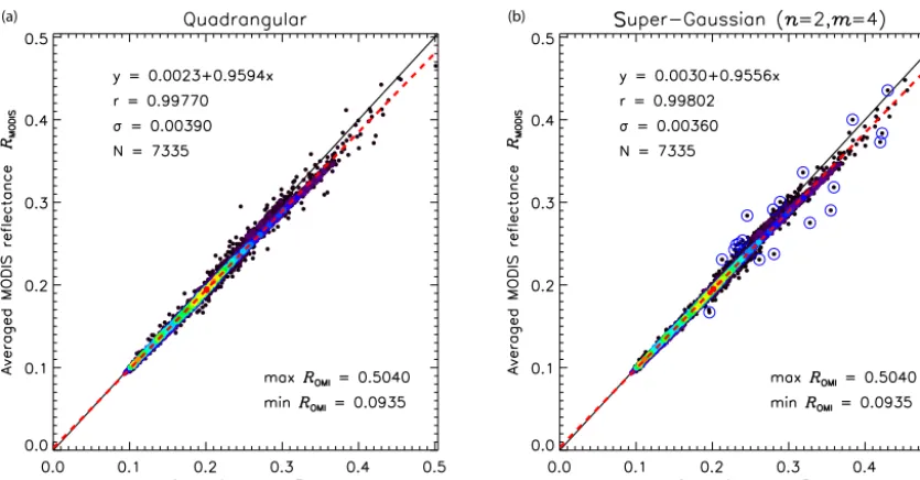
All the 7335 OMI pixels in the scene in Fig. 1 were com-pared to collocated MODIS pixels; see Fig. 3a. Here, all the MODIS pixels that fall (partly) within an OMI quadrangu-lar pixel, as defined by the OMPIXCOR 75FoV corner co-ordinates, are averaged with equal weight, which is the easi-est and quickeasi-est averaging strategy. The MODIS reflectances are somewhat lower than the OMI reflectances; a linear fit through the points shows a slope of 0.959 and an offset of 0.0023. The MODIS reflectances show a Pearson’s correla-tion coefficientr of 0.998 with the OMI reflectances and a standard deviation (SD) of 0.0039. The SD refers to the rms deviation of the measurements to the model fit.
3 OMI point spread function
The true FoV of an OMI pixel is expected to resemble a flat-top Gaussian shape. To investigate the OMI FoV, the re-sponse at 469 nm is compared to the MODIS channel 3 sig-nals, weighted using different super-Gaussian functions in two dimensions and checking the change in the correlation and SD between the OMI and MODIS reflectances. A 2-D super-Gaussian distribution is defined by
g(x, y)=exp
− x
wx n
− y
wy m
, (1)
wherexandyare the along- and across-track directions, and
wx,yare the weights in either direction, defined by
wx=
FWHMx
2(log 2)1/n; wy=
FWHMy
2(log 2)1/m. (2) FWHMx and FWHMy are the full widths at half maximum in the along- and across-track directions, respectively, de-fined in this paper by the 75FoV pixel corner coordinates. The size of the FoV model can be varied to include more or fewer MODIS pixels from neighbouring pixels in the along-and across-track directions by varyingwx andwy. All size changes are reported relative to FWHMxand FWHMy.
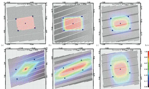
The shape of the FoV model is determined by the Gaus-sian exponentsnandm, which define the “pointedness” of the distribution. In one dimension,n=2 corresponds to a normal distribution,n <2 results in a point-hat distribution, andn >2 results in a flat-top distribution; see the illustration in Fig. 4. Various FoV models are illustrated in Fig. 5. The colours of the square MODIS pixels indicate the relative con-tribution of that pixel. The different panels show OMI pixels at different rows, to illustrate the change in orientation and number of MODIS pixels that fall inside an OMI pixel when the viewing zenith angle (VZA) changes. Fig. 5a shows the quadrangular OMI pixel, with all MODIS pixels within the OMI corner coordinates having equal weight, while all pixels outside the footprint have zero weight. Figure 5b shows a 2-D flat-top super-Gaussian (n=m=8) shape using the 75FoV corner coordinates to constrain the FWHM, resembling the quadrangular shape but with smoother edges. Fig. 5c shows a 2-D super-Gaussian distribution, with n=2 and m=4, which represents the optimal representation of the FoV us-ing a super-Gaussian function. Fig. 5d shows a 2-D point-hat super-Gaussian (n=1, m=1.5) distribution, which is the optimal fit of this function when broken clouds are in the scene. Figure 5e and f show the weights for pixels which are assumed to be twice as wide or long as the 75FoV pixels and using a 2-D super-Gaussian distribution withn=2 and
m=4.
mea-(a) (b)
Figure 3.Scatter plot of OMI and MODIS collocated reflectances for the scene in Fig. 1 using quadrangular OMI pixels(a)and optimised super-Gaussian (n=2,m=4) pixels(b). The red dashed line is the linear least-squares fit to the measurements, given by the linear function y =a0+a1xin the plot.ris Pearson’s correlation coefficient, andσ the standard deviation of the points to the fitted line. The blue-marked points have the largestσ and correspond to the blue OMI pixels in Fig. 1.Nis the number of points, and maxROMIand minROMIthe maximum and minimum value in the plot, respectively.
Figure 4.One-dimensional normalised super-Gaussian distribution functions with varying exponentsn. The normal distribution (n=2) is plotted in blue.
surements, and a constant error for MODIS measurements but weighted by the number of MODIS pixels in each OMI pixel. It shows a reasonably good fit at the optimumn=2.
The red line shows the change in correlation when the along-track width is varied. The shown curve is for the op-timal Gaussian parameters, n=2 and m=4, and peaks at 1.0, meaning that the 75FoV corner coordinates are the op-timal sizes to constrain the FWHM when a super-Gaussian model is used. The lower panel shows the same
dependen-cies in the across-track direction. The change ofr is shown for changingm(the shown blue solid line is for the optimal Gaussian exponentn=2) and the red curve is the width in the across-track direction forn=2 andm=4. The red curve also peaks at 1, again confirming the 75FoV corner coordi-nates, whilempeaks at 4. However, the change for largermis minimal, meaning that the softness of the edges in the across-track direction make very little difference. Only the goodness of fitqdecreases significantly for largerm, som=4 can be used as the optimal parameter. These four optimal parameters are also the absolute maximum in the entire parameter space, withr=0.998. This is noticeably higher than the correlation when quadrangular pixels are used.
The correlation between the OMI and MODIS reflectances and the SD, when the optimal FoV model for this scene is used, is shown in the Fig. 3b. The SD for the optimal FoV is 0.0036. The change in SD for different shapes and sizes is not shown, because it is consistent with the change of the reciprocal of the correlation, in the sense that it is minimal when the correlation peaks and can be equally used to find the optimal FoV characterisation in this way.
3.1 FoV sensitivity
(a) (b) (c) Intensity
(d) (e) (f)
Row number
Row number Row number
Row number Row number
Row number
Figure 5.OMI 75FoV corner coordinates (dark-blue-filled circles), with the OMI centre coordinate (dark blue diamond) and collocated MODIS centre coordinates (black and coloured squares). The colours of the squares indicate the weighting of the MODIS pixels as indicated by the colour bar.(a)Quadrangular weighting, with all MODIS pixels within the corner coordinates having equal weights, everything else disregarded;(b)a 2-D flat-top super-Gaussian distribution with exponentsn=m=8, resembling the quadrangular shape with smoothed edges;(c)a 2-D super-Gaussian distribution withn=2 andm=4;(d)a 2-D point-hat super-Gaussian distribution with exponentsn=1 andm=2;(e)a 2-D super-Gaussian distribution (n=2,m=4) with twice the width in the across-track direction;(f)a 2-D super-Gaussian distribution (n=2,m=4) with twice the width in the along-track direction. Different OMI row numbers are shown (see panel captions) to show the change in orientation and number of MODIS pixels for different rows.
were investigated to show the change in correlation between OMI and MODIS reflectances in time and space.
First, another cloud-free scene was found over the Middle East on 7 October 2008, starting at 10:20 UTC; see Fig. 7. The time difference between OMI and MODIS is about 8 min and 34–45 s. This scene is entirely cloud-free over land, and the reflectance ranges from 0.12 over the ocean to 0.41 over the desert. The correlation between the OMI and MODIS re-flectances is depicted in Fig. 7b, which displays the same de-pendencies as in Fig. 6. The highest correlation (r=0.9977) was found for the same super-Gaussian parameters as before, confirming the optimal OMI FoV model. Only the goodness of fit was slightly lower than before, indicating a lower con-fidence in the correlation.
3.2 Viewing angle dependence
Next, a scene over Australia was selected on 11 October 2008 starting at 04:45 UTC; see Fig. 8. The time difference be-tween OMI and MODIS is about 8 min and 35–43 s. This scene has a large cloud-free part, as well as a large cloudy
part. Most cloud pixels, indicated by the red rectangles, were not used in the analysis. The correlation between OMI and MODIS for various shapes and sizes is again displayed in the right panel. The maximum correlation for this scene was lower than before, r=0.9927, and obtained for a point-hat super-Gaussian distribution with exponentsn=1.5 and
m=2, and FWHM corner coordinates. The goodness of fit is significantly lower than before.
One reason for the lower Gaussian exponents of the 2008 Australian scene in the across-track direction is the removal of the pixels at the end of the swath, which were filtered be-cause of the clouds in those pixels. The OMI FoV is depen-dent on the pixel row, or viewing angle, with wider FoVs at the swath ends. Since most of the cloud pixels are at the swath ends, removing these pixels removes the larger expo-nents. The viewing angle dependence of the FoV is treated here.
(a)
(b)
Figure 6.Pearson’s correlation coefficientrfor OMI and MODIS collocated reflectances in the scene of Fig. 1 as a function of super-Gaussian shape and size of the assumed FoV. The blue line indicates the correlation as a function of exponentn(a)andm(b)for fixed 75FoV corner coordinates. The point marked “Quadr.” marks the correlation for a quadrangular FoV. The red lines are the relation-ships for varying pixel sizes when the optimal Gaussian exponents n=2 andm=4 are chosen. Note that the scales are logarithmic on bothxaxes.
FoV can be distinctly different for FoVs at nadir compared to those with a large VZA. To investigate this effect, the OMI FoV was characterised using a super-Gaussian function de-pendent on VZA. For all the scenes described in this paper, the optimal super-Gaussian shape was determined per OMI pixel row, by varying the Gaussian exponent and determining the maximum correlation between OMI and MODIS pixels for each pixel row. Then the optimal exponents were aver-aged and plotted as a function of pixel row. In this analy-sis, the 75FoV pixel sizes were used to reduce the number of variables and because the above analysis showed that the 75FoV corner coordinates are good indicators of the pixel sizes for Gaussian shapes. The result is shown in Fig. 9. The super-Gaussian exponents are rather wildly fluctuating, be-cause they have a limited sensitivity near the optimum, espe-ciallym. Averaging over the scenes reduces this but is some-what arbitrary. In Fig. 9 a boxcar average over five neigh-bouring points is shown as well.
Still, some change in Gaussian exponents can be observed as a function of VZA. The Gaussian exponent in the across-track directionmchanges from around 3–4 at nadir to about 7 at far off-nadir. Alsonis VZA dependent, changing from about 1.5 at nadir to more than 2 at the swath edges. The reason for the increasing exponents towards the swath edges
is the pixel size increase towards the swath edges. The pixel sizes are shown for reference. FoVs at larger VZA are much wider, changing the optimal super-Gaussian that fit the FoV. Furthermore, as observed before, the diffraction at the edges of the FoV will be different at larger viewing angle.
3.3 Scene dependencies
The smaller Gaussian exponents for the 2008 Australian scene (Fig. 8) are only partly explained by the VZA de-pendence. The Gaussian exponentn <2 indicates a point-hat super-Gaussian distribution in the along-track direction, which is, as Fig. 5e shows, a distribution that is physically unlikely. For this scene, the super-Gaussian function is ap-parently not a good representation of the OMI FoV. The rea-son for this mismatch is broken cloud fields in the scene, which change the scene reflectance between overpasses of Aqua and Aura. Scene dependencies will be investigated be-low.
The overpass time between Aqua and Aura changed in 2008, when a correcting manoeuvre brought OMI closer to MODIS. To illustrate the effect, another Sahara cloud-free scene in the beginning of 2008 was selected, when the ma-noeuvre had not yet been performed; see Fig. 10. The time difference between the instruments for this scene is as large as around 14 min, up to 16 min and 26 s. In this case, the highest correlation is found for a super-Gaussian distribution with exponentsn=1.5 andm=2, which is again a point-hat super-Gaussian distribution. Similarly, when the shape is fixed to the optimal Gaussian exponents, the highest correla-tion is found for pixel sizes that are wider than the 75FoV corner coordinates; see the red curves in Fig. 10. This is different from the reference scene in Fig. 1. The maximum correlation for this scene isr=0.982, which is lower than for the reference scene, in December 2008. The goodness of fit q shows much lower values, showing the difficulty with the used FoV model to correlate the OMI and MODIS reflectances. Apparently, the time difference between Aqua and Aura of 15 min makes a comparison between the two instruments much more challenging, even for almost-cloud-free scenes. It is unlikely that the OMI FoV has changed much between January and December 2008. Furthermore, a cloud-free Sahara scene in 2006 (31 January 2006, around 13:55 UTC, not shown) showed the same lower correlation, peaking for the same Gaussian exponents.
(a) (b)
Figure 7. (a)MODIS RGB scene on on 7 October 2008 at 10:20 UTC over the the Middle East. Yellow and red lines as in Fig. 1, while the individual red OMI pixels are cloud pixels that were manually discarded.(b)Dependence of Pearson’s correlation coefficientrbetween the OMI and MODIS observed reflectance for the scene in the left panel as a function of super-Gaussian shape and size, as in Fig. 6. The optimum in this case was found for Gaussian exponentsn=2 andm=4, and 1×75FoV corner coordinates in both directions.
(a) (b)
Figure 8.Same as Fig. 7 but on 11 October 2008 at 04:45 UTC over Australia. The optimum in this case was found for Gaussian exponents n=1.5 andm=2, and 1×75FoV corner coordinates in both directions. A fit of Gaussian exponentsn=2 andm=4 is best for slightly larger pixels (1.25×75FoV, red line).
where the scene contains broken cloud fields. In the few min-utes between Aqua and Aura overpasses these clouds change shape and position, changing the average reflectance in a pixel when the cloud fraction is changed.
This is the main reason for the small optimal super-Gaussian exponent for the 2008 Sahara scene (Fig. 10) and the Australian scene (Fig. 8): due to scene changes during the different overpass times, the observed overlap function devi-ates from the true FoV, which closely resembles a Gaussian
Figure 9.Super-Gaussian exponentsmandnas a function of OMI pixel row, averaged over all scenes introduced in this paper. The FWHM was fixed to the 75FoV pixel sizes, shown in the lower panel, to determine the optimal exponent. The fat lines are boxcar averages using five points.
3.4 Accuracy of combining OMI and MODIS
The optimal overlap function for MODIS pixels within an OMI FoV can now be determined for practical purposes, i.e. mixed scenes with ocean, land, and clouds. This is needed to determine the accuracy that can be expected when OMI and MODIS measurements are combined to reconstruct the reflectance spectrum for the entire shortwave spectrum. To determine the accuracy, the correlation between collo-cated OMI and MODIS reflectances and the SD was deter-mined by comparing the instruments for the scene shown in Fig. 11. This scene was taken on 13 June 2006, starting on 13:33 UTC, when the time difference between the instru-ments was about 15 min. The scene contains a mixture of land and ocean scenes, with and without clouds, and also smoke from biomass burning on the African continent. Only OMI rows 10–50 were processed, which will often be the case to avoid problems with large pixels or extreme view-ing angles. The optimal correlation was found for super-Gaussian exponents n=1 andm=1.5, and 75FoV corner coordinates (not shown). The low Gaussian exponents can again be explained from the presence of clouds that change the scene between the overpasses, and the exclusion of wide pixels at the swath edges. The correlation between the OMI and MODIS reflectances using this shape is shown in the right panel of Fig. 11. Obviously, the correlation is a lot lower than for cloud-free scenes (r=0.964). The SD is 0.0371, which must be taken into account when OMI and MODIS reflectances are compared or combined. Furthermore, the slope of a linear fit between the OMI and MODIS reflectance
is 0.941, which is smaller than that for cloud-free scenes, which showed about 4 % difference. This larger range in re-flectances for cloud scenes apparently offsets the difference between the instruments even further.
3.5 Geometry differences
The 4–5 % difference between OMI and aggregated MODIS reflectances at 469 nm (Fig. 3) can be governed by changes in viewing and solar conditions between OMI and MODIS. Since the optics and subsatellite points differ for both instru-ments, the viewing angles are slightly different, even if the satellites roughly follow the same orbit. More importantly, since Aura is always behind Aqua, the solar zenith angle for OMI is always different from that of MODIS.
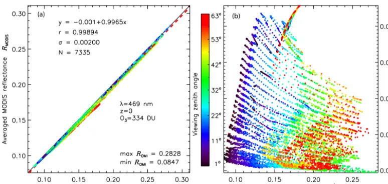
To investigate the effect of the differences in scattering geometry on the measured TOA reflectance, a cloud-free Rayleigh reflectance was modelled for each OMI pixel in the reference scene in Fig. 1. Each pixel was simulated twice, once using the OMI scattering geometry and once using an average MODIS scattering geometry. In this way the ex-pected reflectance difference can be determined due to the difference in overpass time, keeping all else the same. To de-termine the average MODIS reflectance, the simulated radi-ances were averaged over the OMI footprint using the opti-mal flat-top Gaussian distribution withn=2 andm=4, as was determined for this scene (Fig. 6). The average radiance was then divided by the cosine of the solar zenith angle of the MODIS pixel which is closest to the centre of the OMI pixel. In this way, the most representative solar zenith angle is used to normalise the radiances. A realistic surface albedo was taken for each pixel, in order to make the model results com-parable to the observations. The surface albedo database used was the Terra/MODIS spatially completed snow-free diffuse bihemispherical land surface albedo database (Moody et al., 2005). The monochromatic calculations were performed at 469 nm, using a standard Rayleigh atmosphere (Anderson et al., 1986) reaching to sea level and an ozone column of 334 DU. The results are shown in Fig. 12.
re-(a) (b)
Figure 10.Same as Fig. 7 but on 7 January 2008 at 13:45 UTC over the Sahara. The optimum in this case was found for Gaussian exponents n=1.5 andm=2, and 1×75FoV corner coordinates, orn=2 andm=4, and 1.25×75FoV corner coordinates in both directions.
Figure 11.MODIS RGB image on 13 August 2006, around 13:33 UTC (lower part of the image). The yellow lines indicate the MODIS data granules, and the red lines the considered OMI swath, which was from rows 10–50. The optimal correlation between OMI and MODIS for this scene was found for Gaussian exponentsn=1,m=1.5 and 75FoV corner coordinates. The correlation for this pixel shape is shown in the right panel.
flectances. Most likely, calibration differences are causing the difference between the observed reflectances. The sim-ulated correlation and SD are also notably better than for the observed scene. As noted before, clouds have the largest im-pact on the correlation between the observed reflectances of a scene.
4 Conclusions
(a) (b)
Figure 12. (a)Simulated clear-sky reflectances for the reference scene in Fig. 1 using OMI scattering geometries (xaxis) and MODIS geometries (yaxis). The colours indicate the OMI viewing zenith angle of each simulated pixel. The reflectances were simulated at 469 nm, for a standard atmosphere reaching to sea level and an ozone column of 334 DU. The surface albedo was varied according to a database (see text). The underlying red dashed line shows the linear fit to the simulations.(b)Same data as in the left panel but plotted as the relative difference between the OMI and MODIS reflectances.
Due to the design of the OMI CCD detector array and the optical path, the footprint of OMI is not quadrangular and light from successive scans enters the OMI FoV. The shape and size of the FoV was determined for a cloud-free scene, to eliminate, as much as possible, scene changes due to the dif-ferent overpass times of Aura and Aqua. Assuming a super-Gaussian shape with variable exponents and FWHM, the best characterisation of the OMI FoV was found for exponents
n=2 andm=4, and 1×75FoV corner coordinates to con-strain the FWHM.
The OMI FoV changes as a function of viewing angle. When the FWHM are fixed, the Gaussian exponent ranges from about 1.5 at nadir to more than 2 at the swath edges, whilemranges from about 3 to 7. This is mainly due to the increase in pixel size for off-nadir angles. Furthermore, the diffraction at the FoV edges is viewing angle dependent, and the OMI FoV is dependent on polarisation, due to the pres-ence of a polarisation scrambler in the OMI optical path.
The OMI-MODIS overlap function is scene dependent. In particular, for larger time differences between the Aqua and Aura overpasses, the optimal overlap function shape is found for smaller Gaussian exponents and wider overlaps. When the scene changes between overpasses, the signal is spread over a larger area, centred around the centre coordi-nate. Therefore, a more optimal overlap function is found for a point-hat distribution with wider wings. This is especially true for cloud scenes, which are most frequent. The corre-lation decreases and the SD increases when clouds are in the scene, and this can be used as an indication of the ex-pected accuracy of a comparison between OMI and MODIS reflectances. For a scene with broken clouds over both land
and ocean in 2006, optimal Gaussian exponents ofn=1 and
m=1.5 were found. In general, the changes in correlation coefficient are small for small changes of the Gaussian ex-ponents (much smaller than e.g. changes due to time dif-ferences). The true OMI FoV is approximated by a super-Gaussian distribution with exponentn=2 andm=4, and 75FoV corner coordinates.
The use of non-scanning optics like those of OMI will be continued in new instruments, in particular TROPOspheric Monitoring Instrument (TropOMI) on Sentinel-5 (Veefkind et al., 2012), to be launched in 2016. For TropOMI, a cloud masking feature is anticipated from Visible Infrared Imaging Radiometer Suite (VIIRS) on Suomi-NPP (Schueler et al., 2002). Sentinel-5P will fly in “loose formation” with Suomi-NPP, with expected overpass time differences of about 5 min. The results from this study are relevant for that mission, since such an overpass time difference will significantly change the overlap function between TropOMI and VIIRS, and affect the accuracy of a cloud mask from VIIRS. High-resolution VIIRS measurements can be used in the way presented in this paper to study and characterise the TropOMI FoV and the accuracy of the cloud mask.
5 Data availability
Acknowledgements. This project was funded by the Netherlands Space Office, project no. ALW-GO/12-32. Three anonymous referees are thanked for their constructive remarks on the draft manuscript.
Edited by: N. Kramarova
Reviewed by: three anonymous referees
References
Anderson, G. P., Clough, S. A., Kneizys, F. X., Chetwynd, J. H., and Shettle, E. P.: AFGL Atmospheric constituent profiles, Tech. Rep. AFGL-TR-86-0110, Air Force Geophysics Laboratory, 1986.
Bhartia, P. K., McPeters, R. D., Flynn, L. E., Taylor, S., Kramarova, N. A., Frith, S., Fisher, B., and DeLand, M.: Solar Backscatter UV (SBUV) total ozone and profile algorithm, Atmos. Meas. Tech., 6, 2533–2548, doi:10.5194/amt-6-2533-2013, 2013. Bovensmann, H., Burrows, J. P., Buchwitz, M., Frerick, J.,
Noël, S., Rozanov, V. V., Chance, K. V., and Goede, A. P. H.: SCIAMACHY: Mission Objectives and Measure-ment Modes, J. Atmos. Sci., 56, 127–150, doi:10.1175/1520-0469(1999)056<0127:SMOAMM>2.0.CO;2, 1999.
Burrows, J. P., Weber, M., Buchwitz, M., Rozanov, V., Ladstätter-Weißenmayer, A., Richter, A., DeBeek, R., Hoogen, R., Bramstedt, K., Eichmann, K.-U., Eisinger, M., and Perner, D.: The Global Ozone Monitoring Experiment (GOME): Mission Concept and First Scientific Results, J. Atmos. Sci., 56, 151–175, doi:10.1175/1520-0469(1999)056<0151:TGOMEG>2.0.CO;2, 1999.
de Graaf, M., Tilstra, L. G., Wang, P., and Stammes, P.: Re-trieval of the aerosol direct radiative effect over clouds from spaceborne spectrometry, J. Geophys. Res., 117, D07207, doi:10.1029/2011JD017160, 2012.
Fleig, A. J., Bhartia, P. K., Wellemeyer, C. G., and Silberstein, D. S.: Seven years of total ozone from the TOMS instrument-A report on data quality, Geophys. Res. Lett., 13, 1355–1358, doi:10.1029/GL013i012p01355, 1986.
Goddard Earth Sciences Data and Information Services Center: OMI data products and data access, available at: http://disc. sci.gsfc.nasa.gov/Aura/data-holdings/OMI, last access: 1 August 2016.
Goddard Space Flight Center: MODIS data, available at: http:// modis.gsfc.nasa.gov/data/, last access: 1 August 2016.
Kuhlmann, G., Hartl, A., Cheung, H. M., Lam, Y. F., and Wenig, M. O.: A novel gridding algorithm to create regional trace gas maps from satellite observations, Atmos. Meas. Tech., 7, 451– 467, doi:10.5194/amt-7-451-2014, 2014.
Kurosu, T. P. and Celarier, E. A.: OMIPIXCOR Readme File, avail-able at: http://disc.sci.gsfc.nasa.gov/Aura/data-holdings/OMI/ documents/v003/OMPIXCOR_README_V003.pdf, last ac-cess: 6 December 2010.
Levelt, P. F.: OMI Instrument, Level 0-1b processor, Calibration & Operations, in: OMI Algorithm Theoretical Basis Document. Volume I, 2002.
Levelt, P. F., van den Oord, G. H. J., Dobber, M. R., Mälkki, A., Visser, H., de Vries, J., Stammes, P., Lundell, J. O. V., and Saari, H.: The ozone monitoring instrument, IEEE T. Geosci. Remote, 44, 1093–1101, 2006.
Moody, E. G., King, M. D., Platnick, S., Schaaf, C. B., and Gao, F.: Spatially complete global spectral surface albedos: Value-added datasets derived from Terra MODIS land products., IEEE T. Geosci. Remote, 43, 144–158, 2005.
OMI row anomaly team: Background information about the Row Anomaly in OMI, available at: http://projects.knmi.nl/omi/ research/product/rowanomaly-background.php, last access: 26 October 2012.
Schueler, C. F., Clement, J. E., Ardanuy, P. E., Welsch, C., DeLuccia, F., and Swenson, H.: NPOESS VIIRS sen-sor design overview, in: Proc. SPIE, vol. 4483, 11–23, doi:10.1117/12.453451, 2002.