Consequences of Model Misspecification for Maximum Likelihood Estimation with Missing Data

Article

Consequences of Model Misspecification for

Maximum Likelihood Estimation with Missing Data

Richard M. Golden1,* , Steven S. Henley2,3,4, Halbert White5,†and T. Michael Kashner3,4,6 1 _{School of Behavioral and Brain Sciences, GR4.1, 800 W. Campbell Rd., University of Texas at Dallas,}

Richardson, TX 75080, USA

2 _{Martingale Research Corporation, 101 E. Park Blvd., Suite 600, Plano, TX 75074, USA}

3 _{Department of Medicine, Loma Linda University School of Medicine, Loma Linda, CA 92357, USA}

4 _{Center for Advanced Statistics in Education, VA Loma Linda Healthcare System, Loma Linda, CA 92357,}

USA

5 _{Department of Economics, University of California San Diego, La Jolla, CA 92093, USA}

6 _{Office of Academic Affiliations (10X1), Department of Veterans Affairs, 810 Vermont Ave. NW, Washington,} DC 20420, USA

* Correspondence: [email protected]; Tel.:+1-972-883-2423 † _{Halbert White sadly passed away before this article was published.}

Received: 22 October 2018; Accepted: 29 August 2019; Published: 5 September 2019

Abstract: Researchers are often faced with the challenge of developing statistical models with incomplete data. Exacerbating this situation is the possibility that either the researcher’s complete-data model or the model of the missing-data mechanism is misspecified. In this article, we create a formal theoretical framework for developing statistical models and detecting model misspecification in the presence of incomplete data where maximum likelihood estimates are obtained by maximizing the observable-data likelihood function when the missing-data mechanism is assumed ignorable. First, we provide sufficient regularity conditions on the researcher’s complete-data model to characterize the asymptotic behavior of maximum likelihood estimates in the simultaneous presence of both missing data and model misspecification. These results are then used to derive robust hypothesis testing methods for possibly misspecified models in the presence of Missing at Random (MAR) or Missing Not at Random (MNAR) missing data. Second, we introduce a method for the detection of model misspecification in missing data problems using recently developed Generalized Information Matrix Tests (GIMT). Third, we identify regularity conditions for the Missing Information Principle (MIP) to hold in the presence of model misspecification so as to provide useful computational covariance matrix estimation formulas. Fourth, we provide regularity conditions that ensure the observable-data expected negative log-likelihood function is convex in the presence of partially observable data when the amount of missingness is sufficiently small and the complete-data likelihood is convex. Fifth, we show that when the researcher has correctly specified a complete-data model with a convex negative likelihood function and an ignorable missing-data mechanism, then its strict local minimizer is the true parameter value for the complete-data model when the amount of missingness is sufficiently small. Our results thus provide new robust estimation, inference, and specification analysis methods for developing statistical models with incomplete data.

Keywords: asymptotic theory; ignorable; Generalized Information Matrix Test; misspecification; missing data; nonignorable; sandwich estimator; specification analysis

1. Introduction

Researchers are often faced with the challenge of developing statistical models with incomplete data (Little and Rubin 2002;Molenberghs et al. 2014;Rubin 1976). Exacerbating this situation is the possibility

that the researcher’s complete-data model or model of the missing-data mechanism is misspecified. The objective of this article is to formally explore the consequences of model misspecification in the presence of incomplete (missing) data for statistical models that utilize maximum likelihood estimation (MLE) (Fomby and Hill 2003).

Missing Data Problem. The missing data problem is prevalent throughout economics (Abrevaya and Donald 2017;Breunig 2019; Fomby and Hill 1998; McDonough and Millimet 2016;

Miller 2010;Wooldridge 2004). Further, missing data is ubiquitous in other fields of science, engineering (Markovsky 2017), and machine learning (Leke and Marwala 2019). This includes clinical trials and health sciences analyses (e.g., Enders 2010; Little et al. 2012; Molenberghs and Kenward 2007;

Zhou et al. 2014), survey data analysis (e.g., Gmel 2001; Troxel et al. 1998), regression analysis (e.g.,Graham et al. 1997;Greenland and Finkle 1995), verification bias (e.g.,Harel and Zhou 2006;

Kosinski and Barnhart 2003a,2003b), hierarchical modeling (e.g.,Agresti 2002, chp. 12), and mixed modeling (e.g.,Verbeke and Lesaffre 1997). Moreover, latent variable models arising in factor analysis and structural equation modeling contexts (e.g.,Arminger and Sobel 1990;Gallini 1983), hidden Markov chain models (e.g.,McLachlan and Krishnan 1997;Visser 2011), mixed Markov field models (e.g.,

Fridman 2003) and hidden Markov random field models (HMRF) (e.g.,Ryden and Titterington 1998) are interpretable as missing data models where the “hidden states” correspond to the missing data. Additionally, unsupervised and temporal reinforcement learning methods relevant for building sophisticated behavioral learning process models are naturally represented as partially observable Markov decision processes (e.g.,Littman 2009).

Model Misspecification. The problems of estimation and inference in the presence of model misspecification are important for several reasons. First, model misspecification may be present in many, if not most, situations; and so robust methods that address the assumption of correct specification are necessary (White 1980,1982,1994;Golden 1995,1996,2000,2003). While a correctly specified model is always desirable, in many fields such as econometrics, medicine, and psychology, some degree of model misspecification may be inevitable despite the researcher’s best efforts (e.g.,White 1980,1982,1994). Thus, the development and application of robust methods (Golden et al. 2013,2016;Henley et al. 2019) that address the challenges posed by model misspecification (e.g., White 1980, 1982, 1994) has been and continues to be an active area of research (e.g., seeFomby and Hill 2003; Hardin 2003, for relevant reviews). Second, situations arise where the Quasi-Maximum Likelihood Estimates (QMLE) converge to the true parameter value despite the presence of model misspecification. For example, the QMLE can be shown to be consistent to the true parameter value for both linear and nonlinear exponential family regression models even though only the conditional expectation of the response variable given the predictors (covariates) is correctly specified (e.g.,

Gourieroux et al. 1984;Royall 1986;Wedderburn 1974; Wei 1998;White 1994, Corollary 5.5, p. 67). Consistent parameter estimation of the true parameter values of the researcher’s model in the complete data case may also occur for misspecified models where: (i) heteroscedasticity is present (e.g.,Verbeek 2008, sec. 6.3), (ii) the random effects distribution is misspecified in linear hierarchical models (e.g., Verbeke and Lesaffre 1997), or (iii) correlations among dependent observations are misspecified (e.g.,Hosmer and Lemeshow 2000, pp. 315–317;Liang and Zeger 1986;Wall et al. 2005;

Vittinghoffet al. 2012). Third, in more complicated missing data situations, consistent estimation of the true parameter values is possible in linear structural equation models even though only the first two moments have been correctly specified (e.g.,Arminger and Sobel 1990), and in longitudinal time-series modeling even though dependent observations are approximately modeled as independent (Parzen et al. 2006;Troxel et al. 1998;Zhao et al. 1996).

1.1. Maximum Likelihood Estimation for Models with Partially Observable Data

Representing Partially Observable Data Generating Processes. In the selection model framework for representing partially observable data generating processes (Rubin 1976;Little 1994;

(observation) by sampling from the complete-data Data Generating Process (DGP). The complete-data record containing the observation’s values is then decimated by a pattern of missingness sampled from the missing-data mechanism, thus hiding those values in the complete-data record.Rubin(1976) defined three types of missing-data mechanisms. A missing-data mechanism is termed Missing At Random (MAR) when the probability distribution of the pattern of missingness is functionally dependent only upon the observed data. A special case of MAR, called Missing Completely at Random (MCAR), occurs when the probability distribution of the pattern of missingness is not functionally dependent on either observed or unobserved data. Missing data generating processes that are not MAR are termed Missing Not at Random MNAR (i.e., not MAR), also called NMAR. The probability distribution of the pattern of missingness for an MNAR missing-data mechanism is functionally dependent on unobservable data.

A strategy for representing the pattern of missing values in data sets that supports utilizing maximum likelihood estimation is to create a collection of d binary indicator variables, hi =

h

hi,1,. . .,hi,d iT

for the ith data record xi = hxi,1,. . .,xi,d iT

where the notation hi,k = 1 indicates that the kth element of xi, xi,k, is observable and the notation hi,k = 0 indicates that the kth element of xi is not observable. When hi,k = 0, xi,k is typically set equal to a constant such as zero (Allison 2001;Groenwold et al. 2012). This method has been called themissing-indicator method (Groenwold et al. 2012) and has also been called thedummy variable adjustment method(Allison 2001). It provides a useful method for identifying the presence or absence of all the information in the data set and thus is applicable to representing MCAR, MAR, and MNAR missing-data mechanisms. In practice, the researcher often does not have specific knowledge for modeling the joint distribution of the complete-data representation and the missing data indicator variables, which further increases the likelihood of model misspecification. Groenwold et al. (2012) provides some explicit empirical examples illustrating the challenge of correctly applying this approach.

Overview of Parameter Estimation in the Presence of Partially Observable Data. If the missing-data mechanism is MCAR, then maximum likelihood estimation can be utilized by first applying listwise deletion (Allison 2001; King et al. 2001) also known as complete-case analysis (Little and Rubin 2002), which involves simply removing data records (observations) containing missing values from the data set (also seeGroenwold et al. 2012). The resulting dataset, containing no missing values, is then used for statistical modeling. A problem with using listwise deletion to handle a MCAR missing-data mechanism is that the standard errors of the parameter estimates for the researcher’s observable-data model may be larger because the information contained in records with missing values has been removed from the data set. However, a more serious issue with the listwise deletion method is that for MAR data the maximum likelihood estimates may be biased (e.g.,

Allison 2001;Ibrahim et al. 2005;King et al. 2001).

If the missing DGP has a MAR mechanism, then maximum likelihood estimates can be obtained by using Expectation Maximization (EM) (Allison 2001;Dempster et al. 1977;Little and Rubin 2002;

McLachlan and Krishnan 1997) or multiple imputation (MI) (Efron 1994; Groenwold et al. 2012;

Ibrahim et al. 2005; Robins and Wang 2000; Rubin 1996, 1987; Wang and Robins 1998). These algorithms allow for estimation and inference in the presence of missing data while only requiring that the researcher specify the complete-data model. In these situations, it can be shown that the MAR missing-data mechanism is safely “ignorable” in the sense that all of the available information in the data set is used for the purposes of computing unbiased maximum likelihood estimates without the possibility of inflated standard errors (e.g.,Little and Rubin 2002, p. 19) that listwise deletion may cause.

and so cannot be detected without additional assumptions. In addition,Molenberghs et al. (2008) showed that an MNAR model may be replaced with a MAR model that fits the observed data exactly. Further, while statistical tests exist for checking the MCAR mechanism on the data set (e.g.,Little 1988; seeRhoads 2012for a review), tests for the MAR assumption against the MNAR alternative require additional assumptions to be refutable (Breunig 2019;Jaeger 2006;Rhoads 2012). Nonetheless, in practice, much statistical modeling still relies on the assumption of an ignorable missing-data mechanism and thus robust methods that offer improved estimation and inference approaches to deal with models of ignorable missing-data mechanisms are of critical importance. Our theoretical framework provides the foundation for utilizing new model misspecification testing methods (Golden et al. 2013,2016;Henley et al. 2019) to improve statistical modeling on incomplete data in the presence of both ignorable and nonignorable missing data processes.

1.2. Prior Work on Misspecification in Missing Data Models

Although the consequences of model misspecification have been investigated for many years (e.g.,White 1982,1994;Fomby and Hill 2003;Chen and Swanson 2013;Golden et al. 2013,2016), a detailed investigation into the consequences of model misspecification for statistical models in the presence of missing data addressed by this article continues to be an open area of research. It is important to emphasize that when missing data is present, one must not only consider the possibility of misspecification in the complete-data model, but also the possibility of misspecification of the missing-data mechanism. For example, the complete-data model may be correctly specified, but the assumption that the missing-data mechanism is ignorable may be incorrect.

An importantrobustmethod for characterizing the asymptotic distribution of the QMLEs in the presence of model misspecification is the sandwich covariance matrix estimator (e.g.,Huber 1967;White 1982,1994). For example,Arminger and Sobel(1990) used the sandwich covariance matrix estimator for the purpose of characterizing the asymptotic distribution of the QMLEs for linear structural equation models in the presence of missing data.Robins and Wang(2000, pp. 114–115) andSung and Geyer

(2007, pp. 991–92) also used the sandwich covariance matrix estimator as the basis for their analysis of the asymptotic behavior of multiple imputation estimation.Yuan(2009, pp. 1901–2) discusses the relation of the sandwich covariance matrix estimator with respect to missing data problems and model misspecification for Gaussian models. Kashner et al. (2010) used a misspecification-robust difference-in-differences binary logistic regression model with the sandwich covariance matrix estimator applied to “naturally” missing observational data from before–after study designs.

1.3. A Framework for Understanding Misspecification in Missing Data Models

This article provides a formal framework for characterizing models of missing data with ignorable missing-data mechanisms when either the complete-data model is misspecified or the missing-data mechanism is misspecified. First, we provide sufficient regularity conditions on the researcher’s complete-data model to characterize the asymptotic behavior of maximum likelihood estimates in the simultaneous presence of both missing data and model misspecification. These results are then used to derive robust hypothesis testing methods for possibly misspecified models in the presence of ignorable or nonignorable missing-data mechanisms. Second, a method for the detection of model misspecification in missing data problems is discussed using recently developed Generalized Information Matrix Tests (GIMT) (Golden et al. 2013,2016; also see Cho and White 2014;Cho and Phillips 2018;Huang and Prokhorov 2014;Ibragimov and Prokhorov 2017;

conditions that ensure that when the researcher has: (i) correctly specified a probability model for partially observable data as a complete-data model with an ignorable missing-data mechanism, and (ii) the missing data expected negative log-likelihood is convex on the parameter space, then a strict local minimizer of the missing data expected negative log-likelihood is the unique true parameter value for the complete-data model.

To our knowledge, explicit regularity conditions for the new theorems presented here are not readily available in the published scientific literature. Further, methods for testing for model misspecification in the presence of missing values with the GIMT method have not been discussed in the published scientific literature. In the final section of this article, the key results of the stated theorems and their relevance for practical data analysis problems with the use of new model misspecification tests are presented. Sketches of the key proofs which are based upon conventional arguments may be found in the AppendixA.

2. Assumptions

In this section, we provide the assumptions of a formal framework for characterizing models of missing data with assumed ignorable missing-data mechanisms when either the complete-data model or the missing-data mechanism are possibly misspecified.

2.1. Data Generating Process Assumptions

Assumption 1. I.I.D. Partially Observable Data Generating Process. Let (Xi,Hi), i = 1, 2,. . .be a sequence of independent and identically distributed (i.i.d.) random vectors where (Xi,Hi)has a common Radon–Nikodým probability density px,h:Rd× {0, 1}d→[0,∞)defined with respect to a sigma-finite measure νx,h.

In regression modeling applications, the first element of thed-dimensional real vectorxi (a realization ofXi) is a value of the outcome variable for a regression model associated with theith data record while the remaining elements ofxiare values for the predictor variables associated with theith data record,i=1,. . .,n. Theithobserved data indicator recordhi(a realization ofHi) is ad-dimensional binary vector defined so that itsjth element is 1 if thejth element ofxiis observable and thejth element ofhiis 0 otherwise,i=1,. . .,n. Letxn≡[x1,. . .,xn], xn∈Rdn. Lethn≡[h1,. . .,hn], hn∈Ldn. Given thefull partially observable record(x,h), let the number of observable elements ofxbe defined such thatρ(h) ≡ _(1d)T_h,∀_h∈ _Ld _where ρ_{: L}d→ {_{0, 1, 2,}. . ._,d} _{and the notation1dis used to denote a} d-dimensional column vector of ones. For convenience, letρh≡ρ(h). Also define theobservable-data selection matrixs(h)generated byhas a matrix withρhrows anddcolumns such that thekth element of thejth row ofs(h)is equal to 1 if thejth non-zero element inhis thekth element inh; and set thejkth element ofs(h)equal to 0 otherwise. Let y_h: Rd→_Rρh _{be defined such that:y}

h(x) =s(h)x forh∈_Ld\_{0d. Theith observable-data record componenty}

i ≡yhi(xi)is thus aρhi-dimensional column vector generated from the realization of the full partially observable record(Xi,Hi), fori=1. . ., n. Let Yi ≡ yHi(Xi),i = 1, . . ., n. The sequence of random variables Y1,. . .,Yn is i.i.d. because

(X1,H1),. . .,(Xn,Hn)arei.i.d. distributed by Assumption 1. Letyn ≡

n

y₁,. . .,y_noandhn≡ {_h1,. . ._,hn} be realizations ofYn≡ {_Y1,. . ._,Yn}_andHn≡ {_H1,. . ._,Hn}_{respectively. Let(y}n_,hn_{)denote the observed} data sample.

Now define theunobservable-data selection matrixs¯(h)generated byhas a matrix withd−ρ_hrows anddcolumns such that thekth element of thejth row ofs¯(h)is equal to 1 if thejth zero element in his thekth element inh; and set thejkth element ofs¯(h)equal to 0 otherwise. Let zh:Rd→Rd

−_ρh

be defined such that: zh(x) = ¯

s(h)xfor h ∈ _Ld\_{1d. Thus, thed}−ρ_h

i-dimensional column vector zi≡_zh

i(xi)contains the unobservable components associated with theith observed data record,i=1

. . ., n. LetZi≡_zH

Finally, note that the Radon–Nikodým density representation in Assumption 1 is used so that this theory is applicable to not only situations where the complete data vectorXiconsists of discrete or absolutely continuous random variables, but also for situations where the complete data vector Xiincludes both discrete and absolutely continuous random variables. In fact, the Radon–Nikodým densitypx,his also applicable to situations where the elements ofXiare constructed from combinations of both discrete and absolutely continuous random variables. In the special case, whereXiis a vector consisting of only discrete random variables, thenpx,hmay be interpreted as a probability mass function. A common representational convention in the literature (e.g.,Little and Rubin 2002;Orchard and Woodbury 1972, p. 699;Rubin 1976, p. 584;Schenker and Welsh 1988, p. 1553) is to assume that a realization(xi,hi)of an observation can be represented as(zi,yi), which consists of an observable component vectory_i ≡_y

hi(xi)of dimensionρhi and unobservable component vectorzi≡zhi(xi)of dimensiond−ρ_{hi leaving dependence onhi implicit (i} =_1,. . ._{,n). Our Assumption 1 makes the} dependence onhi more explicit and clearly shows how one can apply standardi.i.d. asymptotic statistical theory to support the analysis of missing data problems.

Usingpx,h, definepx(·₎≡R _px,h(·_,h)dν_h(h)andph(·₎≡R _px,h(x,·_)dν_{x(x). Let theobservable-data} density py_h(y_h(x))≡R _px(x)dν_z

h(zh(x)), which can be rewritten using a more implicit compact notation

aspy_h(y_h) ≡ R _px(x)dν_z

h(zh). The density pyh : R

ρh →_[0,∞_{) specifies the conditional probability} distribution of the random vectory_h(X) =s(h)Xgiven a particular observed data indicator record h. Theobservable-data density pyh,h(yh(x),h) ≡

R

px,h(x,h)dνzh(zh(x))specifies the joint probability

distribution of the observed data record (Y,H) that includes the pattern of missingnessHas well as the observable data componentY.

Additionally, define themissing-data mechanism: densityph|_x ≡p_x,h/px. The missingness-data

mechanism is called aMAR missing-data mechanismif there exists a function ph|_yh : Ld×Rρh →[0,∞)

such that p_h|_x(h

x) =ph|yh

h y_h(x)

holds for allh ∈ _Ld_{and for allx} ∈ _Rd_{. A MAR missing-data}

mechanismp_h|_xis calledan MCAR missing-data mechanismif p_h|_x(h

x) =ph(h)holds for allx

∈_Rd_and

for allh∈_Ld_{. A conditional densityp}

h|_xthat is not a MAR missing-data mechanism is called aMNAR missing-data mechanism. These definitions are consistent with the discussion inLittle and Rubin(2002, pp. 11–12; also seeRubin 1976), but are formulated for the specifici.i.d.case considered here.

2.2. Probability Model Assumptions LetsuppXdenote the support ofX.

Assumption 2. Parametric Densities. (i) LetΘbe a compact and non-empty subset of Rr,r∈_{N. (ii) Let} f : Rd×Θ→_[0,∞_{).For each}θ_inΘ_{, f(}·_;θ)is a density with respect toνxand, for eachx∈suppX,f(x;·) is continuous onΘ.(iii) f(x;·_{)is continuously di}ff_{erentiable on}Θ_{for eachx}∈_{suppX.(iv) f(x;}·_{)is twice} continuously differentiable onΘfor eachx∈_suppX.

The approximating complete-data densityf(·_;θ)specifies the likelihood of a data record in the case where no component of the data record is missing for eachθin the parameter spaceΘ. A set of complete-data densities indexed by the parameter vectorθspecifies the researcher’s complete data model: Mc≡f(x;θ):θ∈Θ.

Assumption 3.Ignorable Missing-Data Mechanism. Let qh|_x: Ld×Rd→[0,∞)be a measurable function. (i) For eachx∈_suppX,qh|x(·|_{x)is a density with respect to}ν_{h. (ii) qh|xis MAR.}

Note that the researcher’s approximation to the missing-data mechanism (specified by the density qh|_x) is MAR so thatqh|_xis not functionally dependent upon the unobservable-data record component zh(x). Furthermore,qh|_xis a constant on the parameter spaceΘ. These are the two conditions that

define anignorable missing-datamechanism (e.g.,Little and Rubin 2002, p. 119; also seeHeitjan 1994;

Kenward and Molenberghs 1998;Nielsen 1997;Rubin 1976). Whenqh|_xis MAR, it will be convenient to

define the functionqh|_yhsuch thatq_h|_x(h|x) =q_h|_yh

h y_h(x)

In contrast to Assumption 3, a non-ignorable missing-data mechanism corresponds to a situation where either: (i)qh|_xis functionally dependent upon the unobservable-data record componentz_h(x),

or (ii)qh|_xis not a constant on the complete-data model parameter spaceΘ. Every model of an MNAR

missing-data mechanism is non-ignorable. However, it is possible for a researcher to postulate a non-ignorable MAR or MCAR missing-data mechanism.

In order to specify amissing-data probability model, the researcher constructs a best approximating model of the DGP densitypx,husing the approximating complete-data density f(·;θ)for eachθin

Θtogether with the approximating missing-data mechanismqh|_x. In many practical missing data

applications, it is common practice to only implicitly specify the missing-data probability model since the researcher explicitly provides only the complete-data density f(·_{;θ)and implicitly assumes an} ignorable missing-data mechanism.

Letqx,h ≡ f qh|_x specify the researcher’s best approximating density of the DGP densityp_x,h.

Let H⊆ {_{0, 1}}d_{denote the set of all permissible missing data patterns (i.e., the support ofHi). Let} qh(h;θ)≡

R

qx,h(x,h;θ)dνx(x)andqy_h(y_h(x);θ)≡ R

f(x;θ)dνz_h(zh)for allh∈H. The densityqyh is

intended to approximate the observable-data densitypy_h. The researcher’sobservable-data modelof the data generating process is the set Mo≡

n

qy_h(y_h(x);θ):θ∈Θ_,h∈_Ho_{for a given parameter space}

Θ⊆_Rr_.

The densityqz_h|_y

h,h =

qh|_x/qh|_y

h

f/qy_hspecifies the researcher’s model of the distribution of the missing data given the observable data whenh ∈ _Ld\{_{0d, 1d}}_{. Letqz}

h|yh,h ≡1 forh = 1d(fully

observable case whereqh|_x =q_h|_yh and f =qy_h) andq_zh|_yh,h≡ f forh =0_d(fully unobservable case

whereqh|_x=qh|_yh andqy_h =1).

Definition 1.Misspecified Model.(i) The complete-data modelMcis called a correctly specified complete-data model if the complete-data DGP density px∈_Mcholdsυ_{x-a.e.; otherwiseMcis misspecified complete data model.} (ii) The observable-data modelMois called a correctly specified observable-data model if the observable-data DGP density py_h ∈_Moholdsυ_y

h-a.e.; for allh∈H; otherwiseMois a misspecified observable data model.

Ifpx ∈ _{Mc, then this is a su}ffi_{cient, but not necessary condition for ensuring Mc is correctly} specified. In particular, the statementpx∈_Mcholdsυ_{x-a.e. is a formal way of acknowledging that it} is possible for another densityp..to have the property that its corresponding cumulative distribution function is exactly the same as the cumulative distribution function for the DGP densitypxeven though ..

p(x) =px(x)only for allxwhere the sigma-finite measureνxvanishes. For example, letpx(x) =1 for all|_x| ≤_{1 withpx(x) =0 for all}|_x|>_{1. Letp}.._{(x) =1 for all}|_x|<_{1 withpx(x) =0 for all}|_x| ≥_1. The cumulative distribution functions forpxandp..are identical even thoughpx,

.. p.

A missing-data probability model may be misspecified if either: (i) the complete-data model Mcis misspecified, (ii) the missing-data mechanismqh|_xis misspecified, or (iii) both the complete-data model

Mcand the missing-data mechanismqh|_xare misspecified.

In regression modeling, a complete-data recordxis commonly partitioned such thatx= [R,u]

whereRis the regression model response variable anduis the predictor variables for the regression model. The complete-data probability model is specified byf. Typically, f(x;θ) is factored such that: f(x;θ) = fR|_u

R

u;θR|u

fu(u;θ_u)whereθ=hθ_R|_u,θu i

∈Θ_R|u×Θ_{u. Thus, misspecification of the}

researcher’s complete-data probability model in a regression modeling application may be due to either a misspecification of either (or both) the regression model and the conditional missing predictor variable model. In practice, the researcher’sconditional missing predictor modelis specified by densities of the form fumiss|uobs≡ fu/fuobswhere fuobsis the marginal distribution for the predictors that are fully observable according to the researcher’s missing-data probability model. Additional discussion of conditional missing predictor models may be found inChen(2004) andIbrahim et al.(1999).

2.3. Likelihood Functions, Pseudo-True Parameter Values, and True Parameter Values

Definition 2. Complete-Data Likelihood Function. Assume Assumptions 1, 2(i), and 2(ii) hold. Given a data sample xn, the complete-data likelihood function L_nx:Θ×_Rdn→_[0,∞_{) is defined} such that: Lnx(θ;xn) =

n Q

i=1

f(xi;θ) for all θ ∈ Θ_{. The complete-data negative average log-likelihood}

lnx:Θ×Rdn→[0,∞) is defined such that: l x

n(θ;xn) = −n −₁

logLnx(θ;xn) for all θ ∈ Θ. The complete-data expected negative average log-likelihood lx_:Θ→_[0,∞_{) is defined (when it exists) such that:} lx(θ) = −R _px(x)log(f(x;θ))dνx(x). The complete-data Kullback–Leibler Information Criterion (KLIC)

..

lnx:Θ→[0,∞) is defined (when it exists) such that: ..

lx(θ) =lx(θ) +R px(x)log(px(x))dνx(x).

The complete-data likelihood function (e.g., White 1982,1994; McCullagh and Nelder 1989;

Dobson 2002;Little and Rubin 2002) is the usual likelihood function encountered in problems where no missing data is present. In many situations (e.g., when the complete-data probability model contains members of the linear exponential family), the complete-data expected negative log-likelihood lx(·_):Θ→_[0,∞_{)is convex on the parameter space}Θ_{(e.g.,Kass and Voss 1997, pp. 14–19). In such} situations, a strict local minimizer oflx_{is the unique global minimizer on the parameter space. For} more complicated probability models wherelxcontains multiple strict local and global minimizers, the parameter spaceΘcan sometimes be defined to contain exactly the strict local minimizer oflx.

Definition 3. Complete-Data True Parameter Value. Assume that Assumptions 1, 2(i), and 2(ii) hold. A global minimizer of the complete-data negative average likelihood function lnx(·;Xn):Θ→[0,∞) on the parameter space Θis called a complete-data quasi-maximum likelihood estimator. A global minimizer of the complete-data expected negative log-likelihood lx(·_):Θ→_[0,∞_{) is called a complete-data pseudo-true} parameter valueθ∗_x.A parameter valueθ₀∈Θ_{defined such that for allx}∈_{suppX: fx;}θ₀=px(x)is called a complete-data true parameter value.

Note that when misspecification is present, it is possible that the complete-data true parameter value may not exist because the complete-data model is not capable of representing the complete-data DGP.

For a missing-data probability model, themissing-data likelihood functionis:

Lny,h(θ;yn,hn)≡ n Y

i=1

"Z

qh|_x(hi|xi)f(xi;θ)dνz_h i

zhi(xi)

#

. (1)

when the researcher’s missing-data mechanism model specified byqh|_x(h|x)is an ignorable missing-data

mechanism model (i.e., see Assumption 3) so thatqh|_x(h|x) =q_h|_yh

h yh(x)

, then (1) may be rewritten as:

Lny,h(θ;yn,hn)≡ n Y

i=1 qh|_yh

i

hi

yhi(xi)

Yn

i=1

Z

f(xi;θ)dνzh_i

zhi(xi)

or equivalently as:

Lny,h(θ;yn,hn)≡ n Y

i=1 qh|_yh

i(hi

yi)

n Y

i=1 qy_h

i(yi;θ). (2)

The likelihoodLny,hin (2) shows that when the researcher assumes an ignorable missing-data mechanism model, this implies that the global minimizers ofLny,hare only functionally dependent upon the observable data componentsyn≡_[y

1,. . .,yn]generated from combining the complete-data patternsxn ≡_[x1,. . ._{,xn]and missing-data patternsh}n ≡_[h1,. . ._{,hn]. The global minimizers ofLn}y,h are not functionally dependent on either the researcher’s choice of missing-data mechanismqh|_yh

or an explicit representation of the specific patterns of missingnesshn ≡ [h1,. . .,hn](Rubin 1976;

of an ignorable missing-data mechanism model may be wrong. Thus, maximizing the likelihoodLny,hin (2) to estimate the parameter valuesθwhen the data generating process is MNAR is quasi-maximum likelihood estimation (e.g.,White 1982,1994). These remarks thus motivate the following definition of the observable-data likelihood function (e.g.,Schafer 1997, pp. 11–12;Little and Rubin 2002, p. 119) that is central to the objectives of this article.

Definition 4. Observable-Data Likelihood Function. Assume that Assumptions 1, 2(i), 2(ii), and 3 hold. Let Yn ≡ ×n

i=1R

ρh_{i. Given an observable data sample (y}n_,hn_{), the observable-data}

likelihood function L_ny:Θ×_Yn×_Rdn→_[0,∞_{) is defined such that L}y

n(θ;yn,hn) = n Q

i=1 qy_h

i(yi;θ)where qy_h(y_h(x);θ) = R f(x;θ)dνzh(zh(x))for allθ ∈ Θ. The observable-data negative average log-likelihood

ln:Θ×Yn×Rdn→[0,∞) is defined such that:

l_n(θ;yn,hn) =−_n−1 n X

i=1 logqy_h

i(yi;θ)

(3)

for allθ∈Θ_{. The observable-data expected negative average log-likelihood l:}Θ→[0,∞) is defined (when it exists) by:

l(θ) =−

Z

pyh,h(yh,h)log

qy_h(y_h;θ)dνyh,h(yh,h). (4)

The observable-data negative average log likelihoodlnin general is typically not convex on the parameter spaceΘeven if the complete-data probability model specified by f(x;θ)is a member of the linear exponential family (Orchard and Woodbury 1972;Louis 1982). The non-convex property oflnis a consequence of the Missing Information Principle (seeLouis 1982, and Theorem 3), which states that the Hessian of the observable-data negative average log-likelihood is the difference of two positive semidefinite matrices. McLachlan and Krishnan(1997, pp. 91–95; also seeSchafer 1997, pp. 52–55;

Murray 1977) provide some helpful empirical examples of non-convex missing-data likelihood functions. Thus, in the presence of missing data, it is not unusual for multiple local minimizers, ridges, or multiple global minimizers of the negative average observable data log-likelihood function to exist. To apply the asymptotic theory in such situations, it may be possible to choose the parameter spaceΘ such that l:Θ→_[0,∞_{) is a convex function on}Θ_{and has a unique global minimizer on}Θ_.

Definition 5.Observable-Data True Parameter Value.Assume that Assumptions 1, 2(i), and 2(ii) hold. A global minimizer of the observable-data negative average likelihood function l_non the parameter spaceΘis called an observable-data quasi-maximum likelihood estimator. A global minimizer of the observable-data expected negative log-likelihood l is called an observable-data pseudo-true parameter valueθ∗. A parameter valueθ∗₀∈Θ defined such that for ally_h∈_{suppYh: qy}

h

y_h;θ∗₀=py_h(y_h)for eachh∈_{His called an observable-data true} parameter value.

The observable-data quasi-maximum likelihood estimator is the parameter value that maximizes the likelihood of the observable data in terms of the assumptions associated with the researcher’s proposed probability model. In addition (see Equations (1) and (2)), when the DGP missing-data mechanism is MAR the observable-data pseudo-true parameter value is semantically interpretable as identifying the probability distribution in the researcher’s observable data probability model that is most similar to the probability distribution that generated the observed data (i.e., the distribution specified by the densitypyh,h) using the Kullback–Leibler Information Criterion (e.g.,White 1982,1994;

the observable-data true parameter value and the complete-data true parameter value are identical (see Proposition 3(iii) of this article).

Since the researcher is assuming an ignorable missing-data mechanism, this means that the observable-data pseudo-true parameter value is calculated without incorporating knowledge of the observed patterns of missingness and without incorporating an explicit missing-data mechanism into the researcher’s probability model. These assumptions correspond to potentially serious misspecification errors when the DGP missing-data mechanism is MNAR.

2.4. Moment Assumptions

Let∇_{denote the gradient operator with respect to}θ∈Θ_{yielding anr-dimensional column vector.} Let∇2_{denote the Hessian operator with respect to}θ∈Θ_{yielding anr}×_{rsymmetric matrix. Let the} norm,k · k_{, of anr-dimensional vector}θbe defined such that:kθk2≡θTθ. Letφyh : Rρh×Θ→[0,∞)

be defined such that for ally∈_suppy

h(X)and for allθ∈Θ:φyh(y;θ) =qyh(y;θ)/pyh(y;θ),h∈L

d_.

Let φx: Rd×Θ→[0,∞) be defined such that:φx(x;θ) = f(x;θ)/px(x)for allx∈suppXand for all θ∈Θ_.

Assumption 4.Domination Conditions. For eachh∈_H∪ {_1d}_:

(i) (a) logqy_h is dominated onΘwith respect to py_h; (b) each element of∇_logqy

h is dominated onΘwith respect topyh;

(c) k∇_logqy

hk

2_{is dominated onΘwith respect topy}

h;

(d) each element of∇2_logqy

his dominated onΘwith respect topyh; and

(ii) there exists a finite positive number K such that for allx∈_{suppXand for all}θ∈Θ_{: f(x;}θ)≤_Kpx(x).

Assumption 4 holds under fairly general conditions. Assumption 4(i) corresponds to standard maximum likelihood regularity assumptions applied to the observable probability model representation (e.g.,White 1982,1994;Serfling 1980). Assumption 4(ii) is a relatively weak condition that states the likelihood of an environment events assigned by the researcher’s complete data probability model must have a (generous) upper bound determined by the likelihood of that event in the environment. Simple verifiable conditions for ensuring Assumption 4 holds are: (i) assume that the DGP is bounded (i.e.,|_Xi| ≤_{Kwith probability one for some finite numberK), (ii) logf(x;}θ)is piecewise continuous in its first argument and a twice continuously differentiable function in its second argument, (iii) the parameter spaceΘis a closed and bounded set, and (iv) if for each possible realizationxiin the researcher’s model (i.e., f(x;θ)>0 for allθ∈Θ_{), the realizationxiin the statistical environment} should also be possible with likelihood greater than some positive numberε(i.e.,pe(x)> ε).

2.5. Solution Assumptions

Assumption 5.Uniqueness. (i) For someθ∗∈Θ_{,l has a unique minimum at}θ∗. (ii)θ∗is interior toΘ. The Assumption 5(i) is an identifiability assumption that is commonly made for the purposes of establishing consistency and asymptotic normality for maximum likelihood estimators in the completely observable case (e.g.,White 1982). Assumption 5(i) will fail, for example, if the complete-data model contains redundant or irrelevant parameters (e.g.,White 1982). However, the nature of the actual missing-data mechanism may also cause Assumption 5(i) to fail. For example, there may not be sufficient information in the observed data to uniquely specify how all predictor variables in a regression model covary.

To state our next assumption, letg_yh(y;θ) ≡ −∇_logqy

h(y;θ)and write A(θ) ≡ ∇

2_l(θ)and B(θ)≡R _g

yh(yh;θ)

g_yh(y_h;θ)Tpy_h,h(yh,h)dνy_h,h(yh,h). LetA

∗

Assumption 6(ii) is used in order to apply the Lindeberg–Levy Central Limit Theorem (e.g.,

White 1984, Theorem 5.2). Violations of Assumption 6(i) and Assumption 6(ii) may be interpreted as analogous to the presence of multicollinearity in the special case of linear regression modeling.

3. Theorems

In this section, the explicit regularity conditions developed in Section2are used to formulate and prove key theorems applicable to missing data models comprised of a possibly misspecified complete-data model and a missing-data mechanism that is possibly misspecified as ignorable. Many of the results are applicable to DGPs with either MAR or MNAR missing-data mechanisms.

Theorem 1 establishes conditions for the QMLE to converge to the pseudo-true parameter valueθ∗ even if the complete-data model is misspecified. Theorem 2(i) establishes conditions for the distribution of the quasi-maximum likelihood estimates to have an asymptotic multivariate Gaussian distribution centered atθ∗ with a sandwich covariance matrix even if the complete-data model is misspecified. In addition, Theorem 2(ii) establishes that the Hessian and OPG covariance matrices will differ from each other and the sandwich covariance matrix when the observable-data model is misspecified. This latter result is important for two reasons. First, it suggests alternative methods for estimating the QMLE covariance matrix. Second, Theorem 2(ii) implies that when the Hessian and OPG covariance matrices are not equal that the complete-data model is misspecified regardless of whether or not the researcher has correctly specified the missing-data mechanism as ignorable even if the data is MNAR.

Theorem 3 provides explicit regularity conditions for theOrchard and Woodbury(1972); also see

Louis(1982) Missing Information Principle to hold for ignorable missing-data mechanisms. In addition, Theorem 3 introduces several new forms of the Missing Information Principle that are important for interpreting and computing the covariance matrix of the missing-data maximum likelihood estimates in terms of the researcher’s complete-data model. Proposition 2 establishes conditions for computationally tractable formulas for consistent gradient and covariance matrix estimators. Theorem 4 describes how the shape of the complete-data expected likelihood and the amount of missing information influence the convexity of the expected observable data negative log-likelihood function for both MAR and MNAR environments. Proposition 3 summarizes some key results regarding local and global identifiability of the observable-data pseudo-true parameter values, observable-data true parameter values, and complete-data true parameter values.

3.1. Quasi-Maximum Likelihood Estimation for Possibly Misspecified Missing Data Models

Let themissing-data gradientg¯_n : Rr→_Rr _{be defined such that for all}θ∈Θ_{and for all}(yn,hn)∈ n

× i=1(R

ρh_i)×Ldn_:

¯

g_n(θ;yn,hn)≡_n−1 n X

i=1 g_yh

i

(y_i;θ). (5)

Proposition 1. Missing-Data Average Negative Log Likelihood Function and Gradient Estimation. Assume that Assumptions 1, 2(i), 2(ii), 2(iii), 4(i)a, and 5 hold. Then as n→ ∞_{, ln(}·_;Yn_,Hn₎→_{l and}

¯

g_n(·_;Yn_,Hn₎→_{g uniformly on}Θ_{with probability one. In addition, l andgare continuous on}Θ_.

Theorem 1. Estimator Consistency.Assume that Assumptions 1, 2(i), 2(ii), 4(i)a, and 5 hold. Then as n→ ∞_,θˆ_n→θ∗ with probability one.

3.2. QMLE Asymptotic Distribution for Possibly Misspecified Missing Data Models

Now consider the asymptotic distribution of ˆθ_nwhich is a unique minimizer oflnon a closed and bounded parameter spaceΘthat containsθ∗in the interior ofΘ.

Theorem 2. Asymptotic Distribution of Quasi-Maximum Likelihood Estimates. Assume that Assumptions 1, 2, 4, 5, and 6 hold. (i) As n→ ∞_,

√

nθˆ_n−θ∗converges in distribution to a zero-mean Gaussian random vector with non-singular covariance matrixC∗ ≡_(A∗₎−1_B∗_(A∗₎−1_{. (ii) If, in addition, the} observable-data probability modelMois correctly specified, thenA∗ =B∗.

Theorem 2(i) (whose proof follows directly from the methods ofHuber 1967;White 1982,1994) provides explicit regularity conditions delivering the asymptotic distribution of the quasi-maximum likelihood estimator for possibly misspecified models in the presence of missing data. The covariance matrix of the quasi-maximum likelihood estimate is specified by themissing-data robust covariance matrix(Robins and Wang 2000;Clayton et al. 1998;Arminger and Sobel 1990):

C∗= (A∗)−1B∗(A∗)−1. (6)

Wang and Robins(1998, p. 937) andRobins and Wang(2000, pp. 114–15) simply assume that the conclusions of Theorem1 and Theorem 2 hold in their development of an asymptotic statistical theory of parameter estimation using both single and multiple imputation methods for possibly misspecified models with ignorable missing-data mechanisms. Thus, Theorems 1 and 2 also are useful for providing a set of primitive assumptions for the missing data asymptotic theory of imputation methods developed byRobins and Wang(2000) andWang and Robins(1998).

Theorem 2(ii) provides explicit regularity conditions supporting the assertion that if the observable-data probability model is correctly specified (regardless of the correct specification of the researcher’s missing-data mechanism), then the Information Matrix Equality (A∗ =B∗) holds so thatC∗ can be replaced with either themissing-data Hessian covariance matrixformula (e.g.,Little and Rubin 2002;

Meng and Rubin 1991;Jamshidian and Jennrich 2000):

C∗= [A∗]−1 (7)

or themissing-data OPG (Outer-Product Gradient) covariancematrix (e.g.,Berndt et al. 1974; also see

McLachlan and Krishnan 1997, p. 122) formula:

C∗= [B∗]−1. (8)

Note that the second part of Theorem 2, 2(ii), states that when (6), (7), and (8) are not equivalent (i.e.,C∗ ,[A∗]

−₁

andC∗,[B∗]

−₁

), then the missing-data Hessian covariance matrix formula in (7) and the missing-data OPG covariance matrix formula in (8) are not correct. In this situation, the formula for the missing-data robust covariance matrixC∗in (6) must be used instead of (7) and (8) in order to ensure reliable statistical inferences for possibly misspecified probability models whose parameters are estimated from missing data.

3.3. Validity of Missing Information Principles When Model Misspecification Is Present

The Uniform Law of Large Numbers (e.g., Jennrich 1969, Theorem 2) with Assumptions 1, 2, and 4, provides a variety of convenient ways to estimate A∗, B*, and C∗. Let ˆg_yh =

−R ∇_{logfx; ˆ}θ_nψ_z

h|yh(zh

yh;θ)dνzh(zh). Estimate

B*−1using themissing-data OPG (Outer Product

Gradient) covariance matrix estimator: ˆB−n1≡ n −₁Pn

i=1 ˆ g_yh

i

ˆ g_yh

i

T!−1

matrix estimator: ˆAn≡ ∇2_lnθˆn;yn,hn

, is a convenient estimator for the missing-data robust covariance

matrixC∗given by themissing-data robust covariance matrix estimator: ˆCn≡_Anˆ

−₁

ˆ BnAnˆ

−₁

.

However, in practice, it is desirable to obtain computational formulas for estimating the asymptotic covariance matrix of the parameter estimates C∗ which are expressed in terms of the first and second derivatives of the complete-data probability model Mc ≡ f(x;θ):θ∈Θ rather than the observable-data probability model Mo. In this section, such formulas will be developed for situations where the observable-data model may be misspecified following the classical derivation of the Missing Information Principle which does not explicitly assume that model misspecification may be present (Woodbury 1971;Orchard and Woodbury 1972; also see Louis 1982, eq. 3.1, andMcLachlan and Krishnan 1997, p 100).

Letψz_h|_y

h(zh(x)

yh(x);θ)≡

f(x;θ)

R

f(x;θ)dνz_h(zh(x))forh

∈_Ld\{_0d,1d}_,ψ_z

h|yh(zh(x)

yh(x);θ)≡1 forh= 1d, andψzh|yh(zh(x)

y_h(x);θ)≡ f(x;θ)forh=0d. Note that: R

ψzh|yh(zh(x)

y_h(x);θ)dνz_h(zh(x)) =1

for allθ∈Θ_andy

h(x)∈Rρh.

Proposition 2.Missing-Data Gradient Computation Formulas. Assume that Assumptions 1, 2, 3, and 4 hold. Then, (i)

g_yh(y_h(x);θ) =−

Z

[∇_logf(x;θ)]ψ_zh|_yh(z_h(x)

yh(x);θ)dνzh(zh(x)), (9)

and (ii)

qzh|yh,h(zh(x)

yh(x),h;θ) =qzh|yh(zh(x)

yh(x);θ) =ψzh|yh(zh(x)

yh(x);θ) (10)

Proposition 2(i) provides an expression useful for computing the OPG missing-data covariance

matrix estimator Bn¯ θˆ_n;Yn,Hn !−1

. Moreover, when (9) is used to evaluateg¯_n(θ;yn,hn), then we obtain Equation (2.13) fromOrchard and Woodbury(1972; also seeWoodbury 1971) and Equation (3.1) from Louis (1982). Proposition 2(ii) establishes that the conditional independence relation qzh|yh,h = qzh|yh holds and provides the convenient computational formula for an ignorable-type

complete-data generation model:

qzh|yh,h(zh(x)

y_h(x),h;θ) =

f(x;θ)

R

f(x;θ)dνz_h(zh(x)) .

We now provide formal conditions for Orchard and Woodbury’s Equation (2.15) (Orchard and Woodbury 1972; also see Woodbury 1971) and Louis’s (Louis 1982) Equation (3.2)

to hold by investigating the structure ofAn¯ θˆ_n;Yn,Hn. When they exist, let

e

An(θ;yn,hn)≡ −n −₁

n X

i=1

Z

∇2_logf(xi;θ)ψz_h i

|_y

h_i

zhi

yhi;θ

dνzh_i

zhi

(11)

and

_

An(θ;yn,hn)≡ −n −₁

n X

i=1

Z

∇2_logqz

h_i|yhi

zhi

y_hi;θ

ψz_h

i

|_yh

i

zhi

y_hi;θ

dνz_h

i

zhi

. (12)

When they exist, letAe(θ) ≡ − R R

∇2_logf(x;θ)ψ_z

h|yh(zh

yh;θ)dνzh(zh)pyh,h(yh,h)dνyh,h(yh,h)

and_A(θ)≡ −R R ∇2_logq z_h|_yh(z_h

y_h;θ)ψz

h|yh(zh

y_h;θ)dνzh(zh)pyh,h(yh,h)dνyh,h(yh,h). When it exists, let:

e

Bn(θ;yn,hn)≡ n −₁

n X

i=1

Z

∇_logf(xi;θ)(∇_logf(xi;θ))Tψ_z h_i|yhi

zhi

y_hi;θ

dνz_h

i

zhi

, (13)

which is referred to as theOPG conditional complete-data information matrixwhen A3 holds. Inspecting (13), we see thateBn(θ;yn,hn)is positive semidefinite for allθ. Let

_

g_h(x;θ)≡ ∇_logf(x;θ)−_g

yh(yh(x);θ). (14)

Then, when it exists,

_

Bn(θ;yn,hn)≡ _n−1 n X

i=1

Z _

g_hi(xi;θ)_g_hi(xi;θ)Tψz_h i

|_y

h_i

zhi

yhi;θ

dνzh_i

zhi

, (15)

which is referred to as theOPG conditional missing information matrixwhen Assumption 3 holds. The trace of the positive semidefinite matrix_Bn(·_;yn_;hn_{)defined in (15) may be interpreted as a measure} of the amount of missing data. In the special case where there are no missing data, the trace of (15) vanishes.

LeteB(θ) ≡ R R

∇_logf(x;θ)(∇_logf(x;θ))Tψz_h|_y

h(zh

yh;θ)dνzh(zh)pyh,h(yh,h)dνyh,h(yh,h)and

_

B(θ)≡R R __g h(x;θ)

_

g_h(x;θ)Tψ_z h|yh(zh

yh;θ)dνzh(zh)pyh,h(yh,h)dνyh,h(yh,h)

Theorem 3. Missing Information Principle.

Assume that Assumptions 1, 2, 4, and 5 hold. Then (i)

¯

An(θ;yn,hn) =Ane (θ;yn,hn)− _

An(θ;yn,hn). (16)

andA(θ) =eA(θ)− _

A(θ). In addition, (ii)

¯

Bn(θ;yn,hn) =Bne (θ;yn,hn)− _

Bn(θ;yn,hn), (17)

_

An(θ;yn,hn) =

_

Bn(θ;yn,hn), and (18)

B(θ) =eB(θ)− _

B(θ).

Theorem 3 provides explicit regularity conditions for the Missing Information Principle (MIP) to hold for the case where either (or both) the missing data model is possibly misspecified as ignorable

or the researcher’s complete-data model is misspecified. The formulaA= eA− _

Ain Equation (16) corresponds to the MIP presented in Equation 2.15 fromOrchard and Woodbury(1972; also see

Jank and Booth 2003; McLachlan and Krishnan 1997, pp. 101–3, 111–13; Meng and Rubin 1991). Substituting the relation in (18) into Equation (16) yields an alternative form of the MIP discussed by

Louis(1982, eq. 3.2), which is:An¯ =eAn− _

Bn. Both of these forms of the MIP are valid in the presence of an observable-data model which is possibly misspecified.

If the observable-data model is correctly specified, then the results of Theorem 2(ii) imply that

e

An =eBnwhich may be combined with the results of Theorem 3 to obtain two additional MIPs that

are valid for the case when the observable-data model is correctly specified: An¯ = eBn− _

¯

An =eBn− _

An. To our knowledge, this discussion of these four specific forms of the MIP and their validity in the presence of model misspecification has not been discussed in the literature.

3.4. Detection of Model Misspecification in the Presence of Missing Data

It is important to note that contrapositive of Theorem 2(ii) may be used as the basis for the detection of model misspecification in the observable-data model since Theorem 2(ii) implies that a failure of the Information Matrix Equality indicates the presence of model misspecification in the researcher’s observable-data model. Thus, Theorem 2(ii) suggests a new approach to checking for model misspecification in the presence of missing data for models with assumed ignorable missing-data

mechanisms. If the missing-data Hessian covariance matrix estimatorAnˆ −₁

and the missing-data

OPG covariance matrix estimatorBnˆ −₁

are asymptotically different, then this indicates the presence of model misspecification in the observable-data model.

More specifically, the general theoretical framework for developing Generalized Information Matrix Tests (GIMTs) for the detection of model misspecification (Golden et al. 2013, 2016) may be applied to construct a wide range of entirely new misspecification tests for detecting model misspecification in observable-data models that assume an ignorable decimation mechanism. Further, this method is valid for both MAR and MNAR environments regardless of whether the missing-data mechanism has been correctly specified as ignorable.

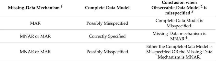
In practice, researchers are often interested in whether the complete-data model, rather than the observable-data model, is misspecified. However, misspecification of the observable-data model when an ignorable missing-data mechanism is postulated implies that either the complete-data model is misspecified or the missing-data mechanism is MNAR. Thus, Theorem 2(ii) in conjunction with the GIMT Framework (Golden et al. 2013,2016) provides a method for the detection of misspecification of complete-data probability models and also provides a method for detecting the presence of an MNAR data generating process in situations where the complete-data model is known, in fact, to be correctly specified.

Nonetheless, it is important to emphasize that the GIMT method is only capable of detecting some types of misspecification of the researcher’s complete-data model. For example, suppose that the complete-data model was misspecified and the missing-data mechanism was correctly specified as ignorable. Situations may exist where the presence of the missingness “hides” misspecification in the observable data model and thus the complete-data model is not identified as misspecified. This occurs because the missing-data mechanism sometimes renders the presence of model misspecification unobservable. Further, this method for detecting model misspecification by checking the Information Matrix Equality cannot directly detect misspecification of the missing-data mechanism because the Information Matrix Equality is not functionally dependent upon the missing-data mechanism. However, misspecification of the missing-data mechanism as ignorable may be indirectly detected by the GIMT method in the special case where the complete-data model isknown to be correctly specified and misspecification is detected in the observable-data model. In this situation, the correctly specified complete-data model (alternative) serves to provide the necessary distribution assumption (Jaeger 2006; Molenberghs et al. 2008; Rhoads 2012) to test for the presence of a nonignorable missing-data mechanism.

3.5. Estimating the Fraction of Missing Information with Possible Model Misspecification

Definition 6.Fraction of Information Loss Functions.(i) The Hessian fraction of information loss function ξA:Θ→R is defined such that for allθ∈Θ: ξA(θ) =λmax

e A(θ)

−₁_ A(θ)

whenAe(θ) −1

exists. The quantityξ∗_A≡ξ_A(θ∗)is called the Hessian fraction of information loss. (ii) The OPG fraction of information loss function ξB:Θ→R is defined such that for allθ∈Θ:ξB(θ) =λmax

e

B(θ)−1_B(θ)

exists. The quantityξ∗_B≡ξ_B(θ∗)is called the OPG fraction of information loss. (iii) The robust fraction of information loss function ξC:Θ→R is defined such that for allθ∈Θ:ξC(θ) =λmax

e

C(θ)_C(θ)

where

_

C(θ) ≡ Ce −₁

(θ)−_C¯

−₁

(θ)when_C(θ) exists. The quantityξ∗_C ≡ ξ_C(θ∗)is called the robust fraction of information loss.

Dempster et al.(1977; also seeMcLachlan and Krishnan 1997; andLittle and Rubin 2002, p. 177) discuss the Hessian fraction of information loss. In particular, they define the fraction of information

loss as the largest eigenvalue ofAe −₁_

Aevaluated at the true parameter values. The OPG and robust fractions of information loss have not been previously discussed in the literature to our knowledge. The Missing Information Principle presented in Theorem 3 provides an interpretation of the Hessian, OPG, and robust fraction of information loss functions, which measure the magnitude of a matrix

relative deviation betweenAe,eBandeC −₁

andA¯,B¯ andC¯ −₁

relative toeA,eBandCe −₁

. This interpretation is valid for environments where the researcher may have misspecified the missing data model as ignorable or misspecified the complete-data model.

Letξ..A(θ) =λmax

e

A(θ)−1_B(θ)

be an alternative representation ofξA(θ)that follows directly from theLouis(1982, eq. 3.2) MIPA=Ae−

_

B.

The fraction of information loss function will typically take on non-negative values that are no greater than one on the parameter space because the parameter space is usually chosen so that the expected negative observed-data log-likelihood function is convex on the parameter space. However, in regions of the parameter space where the expected negative observed-data log-likelihood is not convex (e.g., saddle points), the fraction of information loss function can take on values that are greater than one (Dempster et al. 1977, p. 10;McLachlan and Krishnan 1997, p. 107).

Theorem 4. Fraction of Information Loss and Missing-Data Likelihood Convexity. Assume that Assumptions 1, 2, and 4 hold.

(i) Let θ†be a point in the interior of ΘAssume thateA

θ†is positive definite. BothξA

θ† ≤ _1and ..

ξA

θ†≤_{1if and only if there exists a non-empty open convex subset}Γ_ofΘ_{which contains}θ†such that l is convex onΓ. In addition, the range ofξAand

..

ξAonΓis the set of non-negative real numbers. (ii) Assume thatAe is positive definite on a non-empty open convex subset Γof Θ. Bothξ_A(θ) ≤ 1or

..

ξA(θ)≤1for allθ∈Γif and only if l is convex onΓ. In addition, the range of ξAand ..

ξAonΓis the set of non-negative real numbers.

The assumption thatAeis positive definite on the parameter space is not very restrictive in practice.

Under typically assumed regularity conditions,eAwill be positive definite on the parameter space

Proposition 3.Identifiability.Assume that Assumptions 1, 2(i), 2(ii), and 4(i)(a) hold. LetΓbe a non-empty open subset of the parameter spaceΘ. Assume that the observable-data expected negative log-likelihood l is a convex function onΓ. Letθ∗∈Γ_{be a strict local minimizer of l. Then the following assertions hold.}

(i) The minimizerθ∗is the unique global minimizer of l onΓ.

(ii) If the missing-data mechanism ph|_xis MAR and the observable-data model is correctly specified onΓ, then the unique global minimizerθ∗is the unique observable-data true parameter value for l onΓ.

(iii) If the missing-data mechanism ph|_xis MAR and the complete-data model is correctly specified onΓ, then the unique global minimizerθ∗is both the observable-data true, and complete-data true parameter value for l onΓ.

The assumption thatθ∗ ∈ Γ_{is a strict local minimizer of l means that Assumption 5 holds for} θ∗. In summary, Theorem 4 provides regularity conditions that ensure the observable-data expected negative log-likelihood is convex on the parameter space provided the complete-data expected negative log-likelihood is strictly convex and the amount of missingness is sufficiently small. Given that the observable-data expected negative log-likelihood is strictly convex, then it follows (with some additional regularity conditions) from Proposition 3(iii) that for MAR data any strict local minimizer of the observable-data expected negative log-likelihood is the unique global minimizer and that global minimizer corresponds to the unique complete-data true parameter value.

4. Summary and Conclusions