REAL-ROOTED POLYNOMIALS IN COMBINATORICS

(1)

REAL-ROOTED POLYNOMIALS IN COMBINATORICS Mirkó Visontai

A DISSERTATION in

Mathematics

Presented to the Faculties of the University of Pennsylvania in

Partial Fulfillment of the Requirements for the Degree of Doctor of Philosophy

2012

Supervisor of Dissertation

James Haglund, Professor of Mathematics

Graduate Group Chairperson

Jonathan Block, Professor of Mathematics

Dissertation Committee:

(2)

INFORMATION TO ALL USERS

The quality of this reproduction is dependent on the quality of the copy submitted. In the unlikely event that the author did not send a complete manuscript

and there are missing pages, these will be noted. Also, if material had to be removed, a note will indicate the deletion.

ProQuest LLC.

789 East Eisenhower Parkway P.O. Box 1346

Ann Arbor, MI 48106 - 1346 UMI 3509499

(3)

ACKNOWLEDGEMENT

I am really fortunate to have had Jim Haglund as my advisor. Discussions with him sparked my interest in research early on, and his far-reaching insights and expertise were of tremendous help in making my decisions along the way. I thank him for his constant support throughout the years and for his unobtrusive guidance that kept me on the right track towards reaching my goals.

I owe a lot to the inspiring atmosphere of the math department at Penn as well. The combinatorics class taught by Herb Wilf was one of the most significant influences in my mathematical development. I also benefitted a great deal from the numerous discussions I had with Steve Shatz.

I thank my collaborators, Petter Brändén, Jim Haglund, David G. Wagner, and Nathan Williams. It was a pleasure working with them. I also thank Ira Gessel for discussing his conjecture with me, and Carla Savage for several stim-ulating discussions. Thanks to Robin Pemantle and Martha Yip for serving on my dissertation committee and for their suggestions.

I would also like to thank the staff—Janet, Monica, Paula, and Robin—for alleviating the administrative burden that came with graduate school.

(4)

ABSTRACT

REAL-ROOTED POLYNOMIALS IN COMBINATORICS

Mirkó Visontai James Haglund

Combinatorics is full of examples of generating polynomials that have only real roots. At the same time, only a few classical methods are known to prove that a polynomial, or a family of polynomials, has this curious property. In this dissertation we advocate the use of a multivariate approach that relies on the theory of stable polynomials, which has recently received much attention.

We first present a proof of the Monotone Column Permanent conjecture of Haglund, Ono and Wagner, which asserts that certain polynomials obtained as permanents of a special class of matrices have only real roots. This proof is joint work with Brändén, Haglund and Wagner.

(5)

refinements over Stirling permutations (joint work with Haglund) and for some reflection groups (joint work with Williams). Our approach provides a unifying framework with often simpler proofs.

(6)

Introduction

This dissertation is concerned with generating polynomials in combinatorics whose roots are all real. This is of particular interest due to the deep con-nections between the roots and the coefficients of a polynomial. The body of work presented here was largely motivated by the Monotone Column Perma-nent (MCP) conjecture of Haglund, Ono and Wagner which asserts that certain polynomials obtained from a special class of matrices have only real roots. I was introduced to this conjecture by my advisor, J. Haglund while I was a master’s student at the University of Pennsylvania; see [Vis07].

Chapter 1 of this dissertation contains the proof of MCP conjecture which is based on two papers [HV09, BHVW11]. The first one is joint work with J. Haglund, and contains a multivariate generalization of the conjecture and its proof for n ₆ 4. The multivariate conjecture asserts that a certain multivariate refinement of the polynomials in question is stable, in the sense that it does not vanish whenever all variables lie in the open upper half-plane. The second paper—joint work with P. Brändén, J. Haglund and D. G. Wagner—establishes the multivariate conjecture proposed in the first paper for all n. The techniques from the theory of stable polynomials that were successfully used in the proof of the (multivariate) MCP conjecture are then applied to a related conjecture of Haglund on hafnians. This last, partial, result which appeared in [Vis11], concludes the first chapter.

(9)

Chapter 2 of the dissertation deals with generalizations of the Eulerian poly-nomials and their stable multivariate refinements. This chapter is based on two papers [HV12, VW12]. The first one is joint work with J. Haglund, and gives sta-ble Eulerian polynomials for restricted multiset permutations, such as the Stir-ling permutations. The second one is joint work with N. Williams, and extends the stability results of Eulerian polynomials to groups other than the symmetric group, namely, the hyperoctahedral group, the generalized symmetric group and some affine Weyl groups. The key contribution of this chapter is that the multivariate ideology provides a unifying framework to prove real-rootedness results using stability.

(10)

“. . . the interesting problems tend to be open precisely because the established techniques cannot easily be applied.”

Timothy Gowers

Chapter 1 The MCP conjecture

In this chapter we give a proof of the MCP conjecture. In Section 1.1, we for-mulate the conjecture and briefly mention its history. In Section 1.2, we collect results from the theory of stable polynomials that will be needed for the proof. In Section 1.3, we give the proof of the MCP conjecture—in fact, we prove a stronger multivariate version of it. Finally, we apply some of the techniques used in the proof to a related conjecture of Haglund, and obtain some partial results in Section 1.4.

The results in this chapter are taken from the following three papers [HV09, BHVW11, Vis11]. The main result, presented in Section 1.3, was obtained in collaboration with P. Brändén, J. Haglund and D. G. Wagner. Sections 1.2 and 1.3 are taken verbatim with minor modifications from Sections 2 and 3 of [BHVW11]. Section 1.4 is taken in parts from [Vis11].

1.1 The origin of the conjecture

Let us begin with stating the conjecture. Before we can do that we need to review some definitions.

Definition 1.1.1. Thepermanent of ann-by-n matrix M= (mij)is the “signless

determinant”, that is,

per(M) = X

π∈Sn

n

Y

i=1

mi,πi,

whereSn denotes the symmetric group onnelements.

Definition 1.1.2. An n-by-n matrix A = (aij) is a monotone column matrix if its

entries are weakly increasing down columns, i.e.,aij 6ai+1,jfor all16i6n−1

and all 1₆j₆n.

(11)

Conjecture 1.1.3. LetJndenote the matrix of all ones of sizen-by-n. IfAis an n-by-n

monotone column matrix, thenper(zJn+A), as a polynomial inz, has only real roots.

We will refer to this conjecture as the Monotone Column Permanent (MCP) conjecture. Important special cases of monotone column matrices are the ones with {0, 1} entries, which we call Ferrers matrices. These matrices appear fre-quently in rook theory and in algebraic combinatorics. Haglund, Ono, and Wagner arrived at the MCP conjecture after having settled it for Ferrers ma-trices. In fact, they proved that the so-called hit polynomial of any Ferrers board has only real roots, which is equivalent to the above conjecture for {0, 1} monotone column matrices. Relaxing integrality—much like in the case of the celebrated Heilmann–Lieb theorem—seemed a natural extension. We refer the reader to [HOW99, Hag00, Vis07] for the definition of Ferrers board, hit poly-nomial, and their connection to the Heilmann–Lieb theorem and further details on the history of the problem.

1.2 Theory of stable polynomials

In this section, we introduce elements from the theory of stable polynomials recently developed by Borcea and Brändén. These results lie at the heart of the proof of the MCP conjecture and will be used in Chapter 2 as well.

The basic idea of using a multivariate generalization to prove real-rootedness results is not new. For example, it was applied in one of the beautiful (and probably lesser known) proofs of the Heilmann–Lieb theorem [HL72, Theorem 4.6, Lemma 4.7]. The recent developments in stability-preserving operators, which we are about to discuss, made this approach even more powerful and applicable.

First, we set up some multivariate notation for convenience. For a positive integer n, let [n] denote the set {1, . . . , n} and let x be the shorthand for then -tuple x1, . . . , xn. Similarly, x+y denotes then-tuple x1+y1, . . . , xn+yn. For U a set (or multiset) with entries from [n], we let xU = Q_i_∈_Uxi; for example,

(x+y)[n] ₌ Qn

i=1(xi+yi). The cardinality of U is written |U|. We will denote

the concatenation of x and y by x,y or sometimes by x;y in case we want to emphasize the different roles played byxandy. We useH={w∈_C| =(w)> 0} to denote the open upper half of the complex plane, andHdenote its closure in C. Forf∈C[z]and16j6n, let degzj(f)denote the degree of zj inf.

Definition 1.2.1. A polynomial f ∈ _C[z] is stable if f(z) does not vanish, when-ever the imaginary part of eachzifor16i 6nis positive.

(12)

The results presented here are taken from [BB10, BB09, Brä07]; see also Sec-tions 2 and 3 of [Wag11]. Our presentation is an abridged version of Section 2 of [BHVW11], we repeat the following results and proofs for the sake of com-pleteness with the only difference that most of the theorems are stated for real polynomials only. That suffices for the results in presented in this dissertation. Lemma 1.2.3 (see Lemma 2.4 of [Wag11]). These operations preserve stability of polynomials inR[z].

(a) Permutation:for any permutation σ∈Sn,f7→f(zσ(1), . . . , zσ(n)). (b) Scaling:forc∈_Canda∈_Rn_with_a_>₀_, _f₇_→_cf₍_a

1z1, . . . , anzn).

(c) Diagonalization:for1₆i < j₆n, f→7 f(z)|zi=zj. (d) Specialization:fora∈H, f→7 f(a, z2, . . . , zn).

(e) Inversion:ifdeg_z

1(f) =d,f7→z

d

1f(−z−11, z2, . . . , zn).

(f) Translation:f7→f(z1+t, z2, . . . , zn)∈R[z, t].

(g) Differentiation:f7→∂f(z)/∂z1.

Proof. Only part (f) is not made explicit in [BB10, BB09, Wag11]. But if both z1 ∈Hand t∈H then clearlyz1+t∈H, from which the result follows.

Of course, parts (d), (e), (f), (g) apply to any indexjas well, by permutation. Part (g) is the only difficult one—it is essentially the Gauss-Lucas Theorem. Lemma 1.2.4. Letf(z, t)∈_C[z, t]be stable, and let

f(z, t) =

d

X

k=0

fk(z)tk

withfd(z)6≡0. Thenfk(z)is stable for all06k6d=deg_t(f).

Proof. Clearly fk(z) is a constant multiple of ∂kf(z, t)/∂tk|t=0, for 0 6 k 6 d,

which is stable by Lemma 1.2.3 parts (d) and (g).

Definition 1.2.5. Polynomialsg(z), h(z)∈_R[z]are inproper position, denoted by g h, if the polynomialh(z) +ıg(z)∈_C[z]is stable.

This is the multivariate analogue of interlacing roots for univariate polyno-mials with only real roots.

Proposition 1.2.6 (Lemma 2.8 of [BB09] and Theorem 1.6 of [BB10]). Let g, h ∈

(13)

(a) Thenhgif and only ifg+th∈_R[z, t]is stable.

(b) Thenag+bhis stable for alla, b ∈_Rif and only if eitherhgorg h.

It then follows from parts (d) and (g) of Lemma 1.2.3 that ifhgthen both h andg are stable (or identically zero).

Proposition 1.2.7(Lemma 2.6 of [BB10]). Suppose thatg ∈_R[z]is stable. Then the sets

{h ∈_R[z] :gh} and {h ∈_R[z] :hg}

are convex cones containingg.

Proposition 1.2.8. LetV be a real vector space, φ : Vn _→

R a multilinear form, and e1, . . . , en, v2, . . . , vnfixed vectors in V. Suppose that the polynomial

φ(e1, v2+z2e2, . . . , vn+znen)

inR[z]is not identically zero. Then the set of allv1 ∈V for which the polynomial

φ(v1+z1e1, v2+z2e2, . . . , vn+znen)

is stable is either empty or a convex cone (with apex0) containinge1 and−e1.

Proof. Let Cbe the set of all v1 ∈ V for which the polynomial φ(v1 +z1e1, v2 +

z2e2, . . . , vn+znen)is stable. For v∈ V let Fv =φ(v, v2 +z2e2, . . . , vn+znen).

Since

φ(v1+z1e1, v2 +z2e2, . . . , vn+znen) =Fv1+z1Fe1,

we have C ={v∈ V :Fe1 Fv}. Moreover since Fλv+µw =λFv +µFw it follows from Proposition 1.2.7 that Cis a convex cone provided that Cis non-empty. If C is nonempty then Fv +z1Fe1 is stable for some v ∈ V. But then Fe1 is stable, and so is

(±1+z1)Fe1 =φ(±e1+z1e1, v2 +z2e2, . . . , vn+znen)

which proves that ±e1 ∈C.

(Of course, by permuting the indices Proposition 1.2.8 applies to any indexj as well.)

Definition 1.2.9. A polynomialf∈_R[z]ismultiaffineif it has degree at most one in each variable.

(14)

Proposition 1.2.10 (Theorem 5.6 of [Brä07]). Let f ∈ _R[z]ma _{be multiaffine. Then}

the following are equivalent:

(a) fis stable.

(b) For all1₆i < j₆nand alla∈_Rn_,

∂f ∂zi

(a)∂f

∂zj

(a) −f(a) ∂

2_f

∂zi∂zj

(a)_>0.

Definition 1.2.11. For a linear operator T : _R[z]ma _→

R[z] define its algebraic

symbol as

GT(z,w) =T

(z+w)[n]∈_R[z,w].

The importance of this definition lies in the following characterization of stability-preserving linear operators.

Proposition 1.2.12 (Theorem 2.2 of [BB09]). Let T : _R[z]ma → _R[z] be a linear transformation. Then T preserves stability if and only if either

(a) T(f) =η(f)·pfor some linear functionalη:_R[z]ma →_Rand stablep∈_R[z], or

(b) the polynomialGT(z,w)is stable, or

(c) the polynomialGT(z,−w)is stable.

1.3 Proof of the MCP conjecture

The following multivariate generalization of the MCP conjecture, which ap-peared in [HV09], turned out to be a key idea in the resolution of the conjecture. Conjecture 1.3.1. LetJn denote then-by-nmatrix of all ones, and let

Zn=diag(z1, . . . , zn) =

    

z1 0 · · · 0

0 z2 · · · 0

..

. ... . .. ...

0 0 · · · zn

    

be the n-by-n diagonal matrix of indeterminates z = z1, . . . , zn. If A is an n-by-n

monotone column matrix thenper(JnZn+A)is a stable polynomial.

(15)

1.3.1 Reduction to Ferrers matrices

Lemma 1.3.2. Ifper(JnZn+A)is stable for all Ferrers matricesA, then the MMCPC

(Conjecture 1.3.1) is true.

Proof. If per(zj +aij) is stable for all Ferrers matrices, then by permuting the

columns of such a matrix, the same is true for all monotone column {0, 1} -matrices. Now let A = (aij) be an arbitrary n-by-n monotone column matrix.

We will show that per(zj+aij)is stable bynapplications of Proposition 1.2.8.

LetV be the vector space of column vectors of lengthn. The multilinear form φ we consider is the permanent of ann-by-n matrix obtained by concatenating n vectors inV. Let each ofe1, . . . , enbe the all-ones vector in V.

Initially, let v1, v2, . . . , vn be arbitrary monotone {0, 1}-vectors. Then φ(v1 +

z1e1, . . . , vn+znen) = per(JnZn+H) for some monotone column {0, 1}-matrix

H. One can specialize any number ofvj to the zero vector, and any number ofzj

to1, and the result is not identically zero. By hypothesis, all these polynomials are stable.

Now we proceed by induction. Assume that if v1, . . . , vj−1 are the first j−

1 columns of A, and if vj, . . . , vn are arbitrary monotone {0, 1}-columns, then

φ(v1 +z1e1, . . . , vn +znen) is stable. (The base case, j = 1, is the previous

paragraph.) Puttingvj =0andzj =1, the resulting polynomial is not identically

zero. By Proposition 1.2.8 (applied to index j), the set of vectors vj such that

φ(v1+z1e1, . . . , vn+znen)is stable is a convex cone containing±ej. Moreover,

it contains all monotone {0, 1}-columns, by hypothesis. Now, any monotone column of real numbers can be written as a nonnegative linear combination of

−e1 and monotone {0, 1}-columns, and hence is in this cone. Thus, we may

take v1, . . . , vj−1, vj to be the first j columns of A, vj+1, . . . , vn to be arbitrary

monotone{0, 1}-columns, and the resulting polynomial is stable. This completes the induction step.

After then-th step we find that per(JnZn+A)is stable.

1.3.2 A more symmetrical problem

Let A = (aij) be an n-by-n Ferrers matrix, and let z = {z1, . . . , zn}. For each

1 ₆ j ₆ n, let yj = (zj + 1)/zj, and let Yn = diag(y1, . . . , yn). The matrix

obtained from JnZn+A by factoring zj out of column j for all 1 6 j 6 n is

AYn+Jn−A= (aijyj+1−aij). It follows that

per(zj+aij) =z1z2· · ·zn·per(aijyj+1−aij). (1.3.1)

Lemma 1.3.3. For a Ferrers matrix A = (aij), per(zj +aij) is stable if and only if

(16)

Proof. The polynomials are not identically zero. Notice that=(zj)> 0if and only

if =(yj) ==(1+z−j 1)< 0. If per(zj+aij)is stable, then per(aijyj+1−aij)6=0

whenever=(yj)< 0for all16j6n. Since this polynomial has real coefficients,

it follows that it is stable. The converse is similar.

The set of n-by-n Ferrers matrices has the following duality A 7→ A∨ =

Jn−A>: transpose and exchange zeros and ones. That is, A∨ = (a∨ij) in which

a∨_ij = 1−aji for all 1 6 i, j 6 n. Note that (A∨)∨ = A. However, the form

of the expression per(aijyj +1−aij) is not preserved by this symmetry. To

remedy this defect, introduce new indeterminates x={x1, . . . , xn}and consider

the matrix B(A) = (bij) with entriesbij=aijyj+ (1−aij)xi for all16i, j 6n.

For example, if

A=      

0 1 1 1 1 0 0 1 1 1 0 0 1 1 1 0 0 0 1 1 0 0 0 0 0

     

then B(A) =

     

x1 y2 y3 y4 y5

x2 x2 y3 y4 y5

x3 x3 y3 y4 y5

x4 x4 x4 y4 y5

x5 x5 x5 x5 x5

      .

For emphasis, we may writeB(A;x;y) to indicate that the row variables are x and the column variables arey. The matricesB(A)and B(A∨)have the same general form, and in fact

per(B(A∨;x;y)) =per(B(A;y;x)). (1.3.2) Clearly per(B(A)) specializes to per(aijyj +1−aij) by setting xi = 1 for all

1 ₆ i ₆ n. We will show that per(B(A)) is stable, for any Ferrers matrixA. By Lemmas 1.2.3(d), 1.3.3, and 1.3.2, this will imply the MMCPC.

1.3.3 A differential recurrence relation

Next, we derive a differential recurrence relation for polynomials of the form per(B(A)), for A an n-by-nFerrers matrix. There are two cases: eitherann =0

or ann = 1. Replacing A by A∨ and using (1.3.2), if necessary, we can assume

that ann =0.

Lemma 1.3.4. LetA= (aij)be an n-by-nFerrers matrix withann =0, letk >1be

the number of 0’s in the last column ofA, and letA◦ be the matrix obtained fromAby deleting the last column and the last row ofA. Then

(17)

       

· · 2 · · ·

2 · · · · ·

· · · 2

· · · · 2 ·

· 2 · · · ·

· · · 2 · ·

        7 →        

· · 2 · ·

2 · · · ·

· · · 2 ·

· · · · 2

· 2 · · ·

       

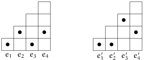
Figure 1.1: σ=3 1 6 5 2 4maps toπ(σ) =3 1 4 5 2.

in which

∂=

nX−k

i=1

∂ ∂xi

+

nX−1

j=1

∂ ∂yj

.

Proof. In the permutation expansion of per(B(A))there are two types of terms: those that do not containyn and those that do. LetTσ be the term of per(B(A))

indexed by σ∈Sn. For each n−k+1 6i 6n, letCibe the set of those terms

Tσ such that σ(i) =n; for a term in Ci the variable chosen in the last column is

xi. Let Dbe the set of all other terms; for a term inDthe variable chosen in the

last column is yn.

For every permutationσ∈Sn, let(iσ, jσ)be such thatσ(iσ) =nandσ(n) =

jσ, and define π(σ) ∈ Sn−1 by putting π(i) = σ(i) if i 6= iσ, and π(iσ) = jσ (if

iσ 6= n). Let Tπ(σ) be the corresponding term of per(B(A◦)). See Figure 1 for an example. Informally,π(σ)is obtained fromσ, in word notation, by replacing the largest element with the last element, unless the largest element is last, in which case it is deleted.

For eachn−k+1₆i₆n, consider all permutationsσindexing terms inCi. The mapping Tσ 7→ Tπ(σ) is a bijection from the terms in Ci to all the terms in per(B(A◦)). Also, for eachσ∈Ci,Tσ =xnTπ(σ). Thus, for eachn−k+16i6n,

the sum of all terms in Ciisxnper(B(A◦)).

Next, consider all permutations σindexing terms in D. The mapping Tσ 7→

Tπ(σ) is (n−k)-to-one from D to the set of all terms in per(B(A◦)), since one needs both π(σ) and iσ to recover σ. Let vσ be the variable in position (iσ, jσ)

of B(A◦). Then vσTσ = xnynTπ(σ). It follows that for any variable w in the set {x1, . . . , xn−k, y1, . . . , yn−1}, the sum over all terms inDsuch thatvσ =wis

xnyn

∂

∂wper(B(A ◦

)).

Sincevσ is any element of the set{x1, . . . , xn−k, y1, . . . , yn−1}, it follows that the sum of all terms in Disxnyn∂per(B(A◦)).

(18)

1.3.4 Proof of the multivariate MCP conjecture

Theorem 1.3.5. For anyn-by-nFerrers matrixA, per(B(A))is stable.

Proof. As above, by replacingA by A∨ if necessary, we may assume that a1n =

0. We proceed by induction on n, the base case n = 1 being trivial. For the induction step, letA◦ be as in Lemma 1.3.4. By induction, we may assume that per(B(A◦)) is stable; clearly this polynomial is multiaffine. Thus, by Lemma 1.3.4, it suffices to prove that the linear transformationT =k+yn∂maps stable

multiaffine polynomials to stable polynomials if k _> 1. This operator has the form T = k+zn

Pn−1

j=1 ∂/∂zj (renaming the variables suitably). By Proposition

1.2.12 it suffices to check that the polynomial GT(z,w) = T

(z+w)[n] = k+zm

mX−1

j=1

1 zj+wj

!

(z+w)[n]

is stable. If zj and wj have positive imaginary parts for all16j6nthen

ξ= k

zm

+

mX−1

j=1

1 zj+wj

has negative imaginary part (since k > 0). Thus zmξ =6 0. Also, zj +wj has

positive imaginary part, so that zj +wj 6= 0 for each 1 6 j 6 n. It follows

that GT(z,w) 6= 0, so that GT is stable, completing the induction step and the

proof.

Proof of the MMCPC. Let A be any n-by-n Ferrers matrix. By Theorem 1.3.5, per(B(A))is stable. Specializingxi=1for all16i 6n, Lemma 1.2.3(d) implies

that per(aijyj+1−aij)is stable. Now Lemma 1.3.3 implies that per(zj+aij) is

stable. Finally, Lemma 1.3.2 implies that the MMCPC is true.

Remark 1.3.6. There are several interesting consequences of the multivariate MCP theorem. These include multivariate stable Eulerian polynomials, a new proof of Grace’s apolarity theorem and some permanental inequalities. We will discuss the Eulerian polynomials in depth in Chapter 2, for the other two results we refer the reader to Section 4 of [BHVW11].

1.4 On a related conjecture of Haglund

(19)

per-fect matchings in a complete bipartite graph. Equivalently, one could consider perfect matchings in the complete graph on even number of vertices instead.

In order to state this conjecture, first we will define this matrix function— the analog of the permanent, and then define a condition on matrices that will replace the monotone column condition.

Definition 1.4.1. Let C = (cij) be a 2n×2na symmetric matrix, the hafnian of

Cis defined as

haf(C) = 1

n!2n

X

σ∈S2n

n

Y

k=1

cσ(2k−1),σ(2k), (1.4.1) whereS2n denotes the symmetric group on2n elements.

Remark 1.4.2. Originally, Caianiello defined the hafnian for (upper) triangular arrays as the “signless Pfaffian” [Cai59, Equation (11)]. There are slight varia-tions in the literature on how to extend the original definition to matrices; the one above is in agreement with the notation in [Hag00].

The analogue of the monotone column property is best explained using tri-angular arrays (which are essentially matrices with the entries below the diago-nal discarded).

Definition 1.4.3. Let 1 ₆ m ₆ n. The mth hook of a triangular array A = (aij)16i<j6n is the set of cells given by

hookm ={(i, m)|i=1, . . . , m−1}∪{(m, j)|j=m+1, . . . , n}. (1.4.2)

Furthermore, the direction alongthemth hook is the one in which the quantity i+j is increasing where(i, j)∈hookm.

Definition 1.4.4. A monotone hook triangular array has real entries decreasing along at leastn−1of its hooks, or possibly along allnof them. Analogously, a

monotone hook matrixis a real symmetric matrix whose entries above the diagonal form a monotone hook triangular array.

We are in position to state the following conjecture of Haglund.

Conjecture 1.4.5 (Conjecture 2.3 in [Hag00]). Let Abe a 2n×2n monotone hook matrix, andJ2n the2n×2nmatrix of all ones. Then the polynomialhaf(zJ2n+A)has

only real roots.

(20)

Threshold graphs have been widely studied and are known to have several equivalent definitions (see Theorem 1.2.4 in [MP95] for a couple). For our pur-poses, the following definition will come in handy.

Definition 1.4.6. A graph G on n vertices is a threshold graph if it that can be constructed starting from a one-vertex graph by adding vertices one at a time in the following way. At step i, the vertex being added is either isolated (has degree 0) or dominating (has degree i−1at the time when added).

Let AG denote the adjacency matrix of a threshold graph G. From

Defini-tion 1.4.1 it is clear, that haf(zJ2n +AG) is invariant under the permutation of

the vertices of G. Hence, we can assume that the vertices of G are labeled in the order of the above construction. This means that in every column i, for 2 ₆ i ₆ 2n, the entries above the diagonal element (i, i) are either equal to z (if vi was added as an isolated vertex) or z+1 (if vi was added as dominating

vertex). This suggests the multivariate generalization that we show next. The idea essentially is to add a new variable for each vertex (see construction of the matrix Bin Theorem 1.4.7 below).

The following theorem is a (multivariate) generalization of the MHH conjec-ture for the special case of adjacency matrices of threshold graphs.

Theorem 1.4.7. Let z1, . . . , z2n denote commuting indeterminates and letB = (bij)

denote the 2n×2n symmetric matrix with entries bij = zmax(i,j). Then haf(B) is a

stable polynomial in the variablesz2, . . . , z2n (z1 only appears on the diagonal).

Proof. The proof is a direct application of the idea of the proof of Theorem 1.3.5. to hafnians. We use induction. Clearly,

haf

z1 z2

z2 z2

=z2

is stable, which settles the base case. Let B◦ denote the (2n−2)-by-(2n−2)

matrix obtained from B by deleting the last two rows and two last columns. Next we show that haf(B) is stable if haf(B◦)was stable. This follows from the differential recursion:

haf(B) =z2nhaf(B◦) +2z2n−1z2n∂haf(B◦)

in which

∂=

2nX−2

i=2

∂ ∂zi

.

(21)

can be seen, analogously to the proof of Theorem 1.3.5, that the algebraic symbol of the linear operatorT =z2n−1z2n

1 z2n−1 +2

P _∂

∂zi

is a stable polynomial. The proposition gives a multivariate version of the MHH conjecture for cer-tain matrices. Unfortunately, it is not clear how to transition from here to the general MHH conjecture. Nevertheless, Theorem 1.4.7 does imply the follow-ing theorem of Haglund, the special case of the MHH conjecture for threshold graphs.

Theorem 1.4.8 (Theorem 2.2 of [Hag00]). Let AG denote the adjacency matrix of a

(non-weighted) threshold graphGon2nvertices. Thenhaf(zJ2n+AG)is stable.

Proof. Let Gbe a threshold graph on 2nvertices. Assume that the vertices of G are ordered as in the definition of the vertex-by-vertex construction above. It is easy to see that matrix B in Theorem 1.4.7 specializes to zJ2n+AG if for all i,

2₆i ₆2n, we set zi =

z, if vi was added as an isolated vertex

z+1, if vi was added as a dominating vertex (1.4.3)

These last operations of translating, specializing and diagonalizing the variables preserves stability by Lemma 1.2.3 parts (c), (d) and (f).

(22)

“Lisez Euler, lisez Euler, c’est notre maître à tous.”

Pierre-Simon Laplace

Chapter 2 Stable Eulerian polynomials

Eulerian polynomials play an important role in enumerative combinatorics. In the context of the MCP conjecture (now theorem), these polynomials naturally arise as permanents of the so-called “staircase” shaped Ferrers matrices. In this chapter, we will examine the combinatorial interpretation of these polynomials in terms of permutation statistics.

We begin with some review of terminology. In Section 2.1, we introduce descents and excedances in permutations. These statistics are often called Eule-rian, since their distribution overSn agrees with the coefficients of the Eulerian

polynomials Sn(x). We then define refinements of these statistics which will

give rise to multivariate Eulerian polynomials. As a consequence of the MMCP theorem these multivariate polynomials are stable which generalizes a classical result that the Eulerian polynomials are real-rooted. This observation serves as a starting point for the results presented in this chapter.

The notion of descent can be extended to various generalizations of per-mutations, such as multi-perper-mutations, or Coxeter groups. Eulerian polyno-mials arising from such generalizations are often known—in some cases only conjectured—to be real-rooted. Our contribution is a unifying framework that allows us to strengthen these results to multivariate stability. This is achieved by understanding the differential recurrences and taking advantage of the fact that they turn out to be given by stability-preserving linear operators.

In Section 2.2, we provide stable Eulerian polynomials for Stirling permuta-tions, and their generalizations. In Section 2.3, we prove stability for Eulerian polynomials for signed and colored permutations and Eulerian-like polynomi-als for some affine Weyl groups.

(23)

2.1 Eulerian polynomials as generating functions

The polynomials

‘‘α = x β = x+x2 γ = x+4x2+x3

δ = x+11x2+11x3+x4

ε = x+26x2+66x3+26x4 +x5

ζ = x+57x2+302x3+302x4+57x5 +x6 etc."

appeared in Euler’s work on a method of summation of series [Eul36].

Since then these polynomials, known as the Eulerian polynomials and their coefficients, the so-called Eulerian numbers have been widely studied in enu-merative combinatorics, especially within the combinatorics of permutations. They serve as generating functions of several permutation statistics such as de-scents, excedances, or runs of permutations. They are intimately connected to Stirling numbers, and also the binomial coefficients, via the famous Worpitzky-identity [Wor83]. See the notes of Foata and Schützenberger [FS70, Foa10], Car-litz ([Car59, Car73]) for a survey and the history of these polynomials.

2.1.1 Statistics on permutations

Letnbe a positive integer, and recall thatSndenotes the set of all permutations

of the set [n] ={1, . . . , n}.

Definition 2.1.1. For a permutationπ=π1. . . πn∈Sn, let

ASC(π) ={i |πi−1 < πi},

DES(π) ={i |πi > πi+1},

denote the ascent setand the descent setofπ, respectively.

For convenience, we will also define a slight variant of the above statistics. Definition 2.1.2. For a permutationπ=π1. . . πn∈Sn, let

ASC0(π) ={i |πi−1 < πi}∪{1},

DES0(π) ={i |πi > πi+1}∪{n},

(24)

Remark 2.1.3. One way to think about the latter extended sets is to consider statistics on the permutation π with a zero prepended to the beginning and a zero appended to the end, i.e.,π0 =πn+1 =0.

Definition 2.1.4. For a permutationπinSn let

des(π) =|DES(π)|

asc(π) =|ASC(π)|

edes(π) =|DES0(π)|

easc(π) =|ASC0(π)|

denote the cardinality of these sets, the number of descents, ascents and ex-tended descents and exex-tended ascents in π, respectively.

Remark 2.1.5. Obviously, edes(π) = des(π) +1 and easc(π) = asc(π) + 1, but sometimes it will be more convenient to use the notation for the extended de-scents (and ade-scents).

We also mention two other well-known permutation statistics. Definition 2.1.6. Let

EXC(π) ={i |πi > i}

denote the set of excedances, and let exc(π) =|EXC(π)|. Definition 2.1.7. Let

WEXC(π) ={i|πi>i}

denote the set of weak excedances, and let wexc(π) =|WEXC(π)|.

It is well-known that excedances are equidistributed with descents, and weak excedances are equidistributed with the extended descents.

2.1.2 Eulerian numbers

Eulerian numbers (see sequence A008292 in the OEIS [OEI12]) denoted by n_k, or sometimes by A(n, k), are amongst the most studied sequences of numbers in enumerative combinatorics. They count, for example, the number of permu-tations of{1, . . . , n}withk extended descents (ork−1 descents).

Definition 2.1.8. For1₆k₆n, let Dn

k E

=|{π∈Sn|edes(π) =k}|. (2.1.1)

(25)

Proposition 2.1.9. For1₆k < n+1,

n+1

k

=k Dn

k E

+ (n+2−k)

n k−1

, (2.1.2)

with initial condition1₁=1and boundary conditionsn_k =0fork₆0orn < k.

In this chapter, we will investigate the ordinary generating function of Eule-rian numbers along with several generalizations of them.

Definition 2.1.10. The generating polynomials of the Eulerian numbers, also known as the classical Eulerian polynomialsare defined as:

Sn(x) = n

X

k=1

Dn k

E

xk = X

π∈Sn

xedes(π) . (2.1.3)

Remark2.1.11. We note here that there is no standard notation for Eulerian poly-nomials unfortunately. In the works of Euler, Carlitz, Comtet the above notation is more prevalent, however, recently the descent generating polynomial (which is off by a factor of x) is also commonly used.

The recursion for the Eulerian numbers (2.1.2) translates into a recursion for the Eulerian polynomials.

Proposition 2.1.12. LetA0(x) =1. Forn>0,

Sn+1(x) = (n+1)xSn(x) +x(1−x)

∂

∂xSn(x). (2.1.4)

Remark2.1.13. See an intuitive proof of this statement in REF (CH3).

This recursion serves as the basis of several proofs of the following folklore result in combinatorics, already noted by Frobenius [Fro10, p. 829].

Theorem 2.1.14. The classical Eulerian polynomial Sn(x) has only real roots.

Fur-thermore, the roots are all distinct and nonpositive.

2.1.3 Polynomials with only real roots

There are several properties of a sequence implied by the fact that its generat-ing polynomial has only real roots. Real-rootedness of a polynomial Pn_i₌₀bixi

with nonnegative coefficients is often used to show that the sequence {bi}i=0...n

is log-concave (b2

i > bi+1bi−1) and unimodal (b0 6 · · · 6 bk > · · · > bn). In

fact, even more is true. For example, the sequence {bi}i=0...n can have at most

(26)

inequalities [New07], Darroch’s theorem [Dar64], etc. Furthermore, the normal-ized coefficients bi/(

P

ibi)– viewed as a probability distribution – converge to

a normal distribution as n goes to infinity, under the additional constraint that the variance tends to infinity [Ben73, Har67]. See also [Pit97] for a review and further references.

2.2 Eulerian polynomials for Stirling permutations

Gessel and Stanley defined and studied the following restricted subset of mul-tiset permutations, called Stirling permutations, in [GS78]. Their motivation was to find a combinatorial interpretation of the coefficients of a polynomial related to the Stirling numbers. Eventually, Stirling permutations turned out to be in-teresting enough combinatorial objects to be studied in their on right.

Definition 2.2.1. Consider the multiset Mn = {1, 1, 2, 2, . . . , n, n}, where each number from 1ton appears twice. Stirling permutationsof ordern, denoted by

Qn, are permutations ofMn in which for all 1 ₆ i ₆ n, all entries between the two occurrences ofi are larger than i.

For instance, Q1 = {11}, Q2 = {1122, 1221, 2211}, and from a recursive con-struction rule—observe thatnandnhave to be adjacent inQn—it is not difficult to see that |Qn|=1·3· · · · ·(2n−1) = (2n−1)!!.

2.2.1 Statistics on Stirling permutations

Gessel and Stanley also studied the descent statistic over Qn (the number of descents gave the interpretations of the coefficients they were looking for). The notions of ascents and descents can be easily extended to Stirling permutations. Bóna in [Bón09] introduced an additional statistic called plateauand studied the distribution of the following three statistics over Stirling permutations.

Definition 2.2.2. Forσ=σ1σ2. . . σ2n ∈Qn, let ASC0

(σ) ={i|σi−1 < σi}∪{1}, DES0

(σ) ={i|σi> σi+1}∪{2n},

PLAT(σ) ={i|σi=σi+1}

denote the set of extended ascents, extended descents and plateaux of a Stirling permutationσ, respectively.

(27)

Definition 2.2.3. Forσ∈Qn, let

denote the number of extended ascents, extended descents, and plateaux in σ.

Remark 2.2.4. edes(σ) +easc(σ) +plat(σ) = 2n+1, for any σ ∈ Qn (since the number of gaps, counting the padding zeros, is exactly2n+1).

We conclude by yet another reason why the extended statistics is a conve-nient shorthand.

Proposition 2.2.5 (Proposition 1 in [Bón09]). The three statistics are equidistributed overQn.

2.2.2 Second-order Eulerian numbers

We adopt the following double angle-bracket notation suggested in [GKP94, p. 256].

Definition 2.2.6. For1₆k₆n, let DDn

k EE

=|{σ∈Qn|edes(σ) =k}|. (2.2.1) Following [GKP94], we refer to these numbers as the “second-order Eulerian numbers”1 since they satisfy a recursion very similar to (2.1.2).

Proposition 2.2.7(Equation (14) in [Car65]). For1₆k < n+1, we have

n+1 k

=kDDn k

EE

+ (2n+2−k)

n k−1

, (2.2.2)

with initial condition1₁=1and boundary conditionsn_k =0fork₆0orn < k. Remark2.2.8. Note that our indexing is in agreement with sequence A008517 in [OEI12] and with the definition of the statistics adopted from [Bón09], however it differs from the one in [GKP94].

The second-order Eulerian numbers have not been as widely studied as the Eulerian numbers. Nevertheless, they are known to have several interesting combinatorial interpretations. Apart from counting Stirling permutations Qn with kdescents [GS78], kascents, kplateau [Bón09], these numbers also count

(28)

the number of Riordan trapezoidal words of length n with k distinct letters [Rio76, p. 9], the number of rooted plane trees on n+1 nodes with k leaves [Jan08], and matchings of the complete graph on 2n vertices with (n−k) left-nestings (Claim 6.1 of [Lev10]).

Definition 2.2.9. Thesecond-order Eulerian polynomial, denoted byS(n2)(x), is the

generating function of the second-order Eulerian numbers, formally,

S(_n2)(x) =

n

X

k=1

DDn k

EE

xk = X

σ∈_Qn

xedes(σ).

The following theorem is an analog of Theorem 2.1.14 for the second-order Eulerian numbers.

Theorem 2.2.10 (Theorem 1 of [Bón09]). The second-order Eulerian polynomial

S(n2)(x)has only real (simple, nonnegative) roots.

This result can be seen as the consequence of that the following recursion satisfied by these generating polynomials which is strikingly similar to (2.1.4). Proposition 2.2.11(Equation (13) in [Car65]). LetS(₁2)(x) =1.Forn_>0,

S(_n2₊)₁(x) = (2n+1)xS(_n2)(x) +x(1−x) ∂

∂xS (2)

n (x). (2.2.3)

2.2.3 A stable refinement of the classical Eulerian polynomial

Brändén and Stembridge suggested finding a stable multivariate generalization of the Eulerian polynomials. In [HV09], the multivariate polynomial

Sn(x) =

X

π∈Sn Y

πi>i xπi

!

, (2.2.4)

was shown to be stable for n₆5, and was conjectured to be stable for all n. Next we show that the multivariate refinement in (2.2.4) refines the weak ex-cedance set and the extended descent set statistics simultaneously. See Propo-sition 2.2.13 below for a formal statement. This correspondence is key as the extended descents allow for an easy recurrence. So, for convenience, we will be working with extended descents instead of weak excedances.

Let us continue with the introduction of some notation for the refinement of the extended descent sets.

(29)

and similarly, let its ascent topset be

AT(π) ={πi+1 :06i 6n+1, πi< πi+1},

whereπ0 =πn+1 =0.

Proposition 2.2.13(Proposition 3.1 in [HV12]).

Sn(x) =

X

π∈Sn

xDT(π),

Proof. Follows from a bijection of Riordan [Rio58, page ], see also Theorem 3.15 of [Bre94].

Following the idea of P. Brändén for the proof of stability of typeAEulerian polynomials (given in detail in Section 2.3.2) consider the following homoge-nization ofSn(x):

Sn(x,y) =

X

π∈Sn

xDT(π)yAT(π). (2.2.5) Theorem 2.2.14(Theorem 3.2 of [HV12]). Sn(x,y)is a stable polynomial.

Proof. S1(x1, y1) =x1y1 which is stable. Note that the following recursion

Sn+1(x,y) =xn+1yn+1∂Sn(x,y), (2.2.6)

holds for n_> 1, where∂again denotes the sum of all partials. Note that∂is a stability preserving operator by Proposition 1.2.12, since its algebraic symbol

G∂ =

n

X

i=1

1 xi+ui

+

n

X

i=1

1 yi+vi

!

(x+u)[n](y+v)[n]

is a stable polynomial.

We will often deal with functions that havexand yas variables, and so un-less specified otherwise the special symbol∂will always denotePni=1

∂ ∂xi +

∂ ∂yi

, the sum of partial derivatives with respect to allx andyvariables.

Remark2.2.15. Using the ascent tops and descent tops for subscripts in the mul-tivariate refinement is crucial. If we were to use the position of descents and ascents as subscripts, the resulting polynomials would fail to be stable.

From Theorem 2.2.14 we get the following corollary, which is also a special case of Theorem 3.4 of [BHVW11] for Ferrers boards of staircase shape.

(30)

In [BHVW11] the stability results for staircase shape boards were further extended to obtain a stable multivariate generalization of the multiset Eulerian polynomial previously studied by Simion [Sim84]. We continue along a similar direction as well, and extend Theorem 2.2.14 to a restricted subset of multiset permutations introduced in this section, the Stirling permutations.

2.2.4 Multivariate second-order Eulerian polynomials

Janson in [Jan08] suggested studying the trivariate polynomial that simultane-ously counts all three statistics of the Stirling permutations (see also [Dum80]):

S(_n2)(x, y, z) = X

σ∈_Qn

xdes(σ) yasc(σ) zplat(σ). (2.2.7)

We go a step further, and introduce a refinement of this polynomial obtained by indexing each ascent, descent and plateau by the value where they appear, i.e., ascent top, descent top, plateau:

S(_n2)(x,y,z) = X

σ∈_Qn

xDT(σ)yAT(σ)zPT(σ), (2.2.8) whereAT(σ)andDT(σ)are extended to Stirling permutationsσin the obvious way and the plateaux top set is defined asPT(σ) ={σi :σi =σi+1}. For example,

S(₁2)(x,y,z) =x1y1z1,

S(₂2)(x,y,z) =x2y1y2z1z2+x1x2y1y2z2 +x1x2y2z1z2.

These polynomials are multiaffine, since any value v ∈ {1, . . . , n} can only appear at most once as an ascent top (similarly, at most once as a descent top or a plateau, respectively). This is immediate from the restriction in the definition of a Stirling permutation. Furthermore, each gap (j, j+1) for 0 ₆ j ₆ 2n in a Stirling permutation σ ∈Qn is either a descent, or an ascent or a plateau. This implies thatS(n2)(x,y,z)is also homogeneous, and of degree2n+1.

Theorem 2.2.17. The polynomialS(n2)(x,y,z)defined in(2.2.8)is stable.

Proof. Note that

S(_n2₊)₁(x,y,z) =xn+1yn+1zn+1∂Sn(2)(x,y,z), (2.2.9)

where∂=Pn_i₌₁∂/∂xi+

Pn

i=1∂/∂yi+

Pn

i=1∂/∂zi.The recursion follows from

the fact that each Stirling permutation in Qn+1 is obtained by inserting two

(31)

the statistic—either ascent, plateau, or descent—that existed in the gap before. From here, the proof is analogous to that of Theorem 2.2.14.

There are some interesting corollaries of this theorem. First, note that, di-agonalizing variables preserves stability (see part c in Lemma 1.2.3). Hence, by setting x1 = · · · = xn = x, y1 = · · · = yn = y, and z1 = · · · = zn = z, we

immediately have the following.

Corollary 2.2.18. The trivariate generating polynomialS(n2)(x, y, z)defined in(2.2.7)

is stable.

Specializing variables also preserves stability (part d of Lemma 1.2.3). Thus, by setting y=z=1, we get back Theorem 2.2.10.

If we specialize variables first, without diagonalizing, namely sety1 =· · ·=

yn=z1 =· · ·=zn =1we get a different corollary.

Corollary 2.2.19. The multivariate descent polynomial for Stirling permutations

S(_n2)(x) = X

σ∈Qn

xDT(σ) (2.2.10)

is stable.

Corollary 2.2.20 (Theorem 2.1 of [Jan08]). The trivariate polynomial S(n2)(x, y, z)

defined in (2.2.7)is symmetric in the variablesx,y,z.

Proof. Follows from the symmetry of the recursion (2.2.9) and the fact that

S(₁2)(x, y, z) =xyz.

2.2.5 Generalized Stirling permutations and Pólya urns

One can model the differential recursion in (2.2.9) as follows (see the Urn I model in [Jan08]). Step 1: start with r = 3 balls in an urn. Each ball has a different color: red, green, blue. At each step i, for i =2 . . . n, we remove one ball (chosen uniformly at random) from the urn and put in three new balls, one of each color. The distribution of the balls of each color corresponds to the distribution of the ascents (red), descents (green), and plateau (blue) in a Stirling permutation. Our multivariate refinement can be thought of as simply labeling each ball by a number i that represents the step i when we placed the ball in the urn. Clearly, this method can be further generalized torcolors, as was done by Janson, Kuba and Panholzer in [JKP11], which led them to consider statistics over generalizations of Stirling permutations.

(32)

Definition 2.2.21. Let r and n be a positive integers. The set of r-Stirling per-mutations of order n, denoted by Qn(r), is the set of multiset permutations of

{1r, . . . , nr}with the property that all elements between two occurrences ofiare at leasti. In other words, every element that appears between “consecutive” oc-currences of i is larger thani, or in pattern avoidance terminology,Qn consists of multiset permutations of {1r, . . . , nr}that are212-avoiding.

Janson, Kuba and Panholzer in [JKP11] considered various statistics over r-Stirling permutations. We define the ascent top sets and descent top sets identically as in the two previous sections (with the convention of padding with zeros, σ0 = σrn+1 = 0). In addition, we will adopt their definition of the j

-plateau, and define the analogousj-plateau top set.

Definition 2.2.22. For anr-Stirling permutationσ, aj-plateau top setofσ, denoted by PTj(σ), is the set of values σisuch that σi =σi+1 whereσ1. . . σi−1 contains

j−1instances ofσi.

In other words, aj-plateau counts the number of times thejth occurrence of an element is followed immediately by the (j+1)st occurrence of it. We note that there arej-plateaux for j=1 . . . r−1 inQn(r).

Now we can define a multivariate polynomial that is analogous to the pre-viously studied S(n1)(x,y)and Sn(2)(x,y,z). Forr>1, let

S(_nr)(x,y,z1, . . . ,zr−1) =

X

σ∈_Qn(r)

xDT(σ)yAT(σ)

r−1

Y

j=1

zPT_j j(σ) (2.2.11) wherezj =zj,1, . . . , zj,n for all j=1, . . . , r−1.

Theorem 2.2.23. S(nr)(x,y,z1, . . . ,zr−1)is a stable polynomial.

Proof. The proof is identical to that of Sn and S(n2) (see Theorems 2.2.14 and

2.2.17) and therefore omitted.

As a corollary of this theorem, we obtain that the diagonalized polynomial,

S(nr)(x, y, z1, . . . , zr−1) is symmetric in the variables x, y, z1, . . . , zr−1 which

im-plies the results of Theorem 9 in [JKP11]. Analogously, we could define the rth order Eulerian numbers as the number ofr-Stirling permutations with exactlyk descents (or equivalently, kascents or k j-plateau for some fixedj). We suggest the notationn_k_r, rbeing the shorthand for therangle parentheses. The results for the special cases of r = 1 and r = 2 give the results for permutations and Stirling permutations, respectively.

(33)

Definition 2.2.24. Let k1, . . . , kn be nonnegative integers. The set of generalized

Stirling permutations of rank n, denoted by Q∗n, is the set of all permutations of

the multiset {1k1_{, . . . , n}kn} _{with the same restriction as before: for each} _i_{, for} 1₆i ₆n, the elements occurring between two occurrences ofi are at leasti.

We can further generalize the multivariate Eulerian polynomials by simply extending the above defined statistics to generalized Stirling permutations. This corresponds to an urn model with balls colored withκ=maxn

i=1ki+1many

col-ors: c1, c2, . . . , cκ. We start withk1+1balls in the urn colored withc1, . . . , ck1+1

(each ball has a different color). In each round i, for 2 ₆i ₆ n, we remove one ball and put inki+1balls, one from each of the firstki+1colors,c1, . . . , cki+1.

We can then define a multivariate polynomial counting all statistics simultane-ously,

S(∗)_n (x,y,z1, . . . ,zκ−2) =

X

σ∈_Q∗

n

xDT(σ)yAT(σ)

κ−2

Y

j=1

zPT_j j(σ) (2.2.12) Theorem 2.2.25. S(∗)n (x,y,z1, . . . ,zκ−2)is stable.

Proof.

S(∗)_n₊₁(x,y,z1, . . . ,zλ−1) =xn+1yn+1

knY+1−1

`=1

z`,n+1

!

∂S(∗)_n (x,y,z1, . . . ,zκ−2),

whereλ=max(κ−1, kn+1), and∂, as before, denotes the sum of all first-order

partials (with respect to all variables inS(∗)n ).

Theorem 2.2.23 is a special case of Theorem 2.2.25 withki=r, for all16i6

n. Note that the diagonalized version of the polynomial defined in (2.2.12) need not be a symmetric function in all variablesx, y, z1, z2, . . . zκ−2. Nevertheless, if

we specialize all variables except x, i.e., by lettingy = z1 = · · · = zκ−2 = 1 we

get the following result of Brenti.

Theorem 2.2.26 (Theorem 6.6.3 in [Bre89]). The descent generating polynomial over generalized Stirling permutations

S(∗)_n (x) = X

σ∈Q∗

n

xedes(σ)

has only real roots.

(34)

in each round. This way, we could define (r, s)-Eulerian numbers, polynomials, and investigate whether they are stable or not.

Several related questions concerningq-analogs, Legendre–Stirling numbers, Durfee squares are posed in [HV12].

2.3 Stable

W

-Eulerian polynomials

In this section, we discuss how the stability results of the Eulerian polynomi-als can be further extended in another direction. Reiner [Rei93, Rei95] and Brenti [Bre94] noted that the notion of descent can be defined for groups other than the symmetric groups. In this section we focus mainly on Coxeter groups. We begin by revising some basic Coxeter group terminology, and show how descents can be defined in such groups. That is essentially all we need to define the so-calledW-Eulerian polynomials, which we will denote as P(W;x) follow-ing Brenti (mainly to avoid confusion between the typeAEulerian polynomials and the classical ones).

Brenti showed that the type B Eulerian polynomials have only real roots and conjectured that for any Coxeter group W, the W-Eulerian polynomial is real-rooted. We follow our multivariate approach. In particular, we de-fine rede-finements of the descent statistics that will give rise to stable multivari-ate W-Eulerian polynomials for some W. For type A, we present Brändén’s proof [Brä10]. We then show how this can be extended to type B (hyperoctahe-dral group or signed permutations), generalizing the univariate result of Brenti. With a little more work we give a stable refinement for the generalized symmet-ric group (colored permutations). Finally, we show stability results for affine Eu-lerian polynomials, introduced by Dilks, Petersen, and Stembridge in [DPS09]. Our multivariate stability results generalize the already known univariate real-rootedness results, but we are not able to settle the cases where real-real-rootedness is only conjectured (see Conjectures 2.3.3 and 2.4.3, and Remark 2.4.9).

2.3.1 Eulerian polynomials for Coxeter groups

We follow the notation in [BB05]. Let S be a set of Coxeter generators, m be a Coxeter matrix, and

W =hS: (ss0)m(s,s0) =e, fors, s0 ∈S, m(s, s0)<∞i

be the corresponding Coxeter group. Given such a Coxeter system (W, S) and σ∈W, we denote by `W(σ)the length ofσinW with respect toS.

Definition 2.3.1. ForW a finite Coxeter group, the descentset ofσ∈W is

(35)

Definition 2.3.2. ForW a finite Coxeter group, theW-Eulerian polynomialis the descent generating polynomial

P(W;x) = X

σ∈W

x|DW(σ)|.

The study of these polynomials was originated by Brenti, who also made the following conjecture.

Conjecture 2.3.3 (Conjecture 5.2 of [Bre94]). For every finite Coxeter groupW, the polynomialP(W;x)has only real roots.

2.3.2 Stable Eulerian polynomials for type

A

Let An denote the Coxeter group of type A of rank n. We can regard An as

Sn+1, the group of all permutations on[n+1] with generatorsS={s1, . . . , sn},

wheresi is the transposition(i, i+1)for 16i 6n.

Proposition 2.3.4(Proposition 1.5.3 in [BB05]). Givenσ=σ1. . . σn+1 ∈An, DA(σ) ={si∈S:σi > σi+1},

Definition 2.3.5. TheEulerian polynomials of type Aare defined as P(An;x) =

X

σ∈An

x|DA(σ)|. Using this notation we have that

P(An;x) =

Sn−1(x)

x ,

whereSn(x)denotes the classical Eulerian polynomial defined in Definition 2.1.10.

Hence, by Theorem 2.1.14, we immediately have the following. Theorem 2.3.6. P(An;x)has only real roots.

To give a multivariate refinement of this polynomial we make use of follow-ing refined typeAstatistics.

Definition 2.3.7. Given σ∈An, define the typeAdescent topset to be DTA(σ) ={max(σi, σi+1) :16i6n, σi> σi+1},

and similarly, let the typeAascent top set be

(36)

Remark2.3.8. This definition is slightly different from the descent top set defined in Definition 2.2.12 for extended descents. For example, when σ =31452∈ A4, DTA(σ) ={3, 5}and ATA(σ) ={4, 5}.

Note the seemingly superfluous notation max(σi, σi+1)simply reduces toσi

and σi+1 in the case of type Adescent top and ascent top sets, respectively. Its

significance will become apparent when we introduce the type B descent top and ascent top sets (see Definition 2.3.15).

Theorem 2.3.9(Brändén [Brä10]). P(An;x,y) =

X

σ∈An

xDTA(σ)yATA(σ) (2.3.1)

is stable.

Proof. We proceed by induction. Note that P(A0;x1, y1) = 1 is stable. By

ob-serving the effect of inserting n+1into a permutation σ∈An−1 on the type A

ascent top and descent top sets, we obtain the following recursion. For n > 0, we have

P(An;x,y) = (xn+1 +yn+1)P(An−1;x,y) +xn+1yn+1∂P(An−1;x,y). (2.3.2)

We remind the reader here that ∂ = Pn_i₌₁_∂x∂

i +

∂ ∂yi

. It is easy to check using Proposition 1.2.12 that the linear operatorT = (xn+1+yn+1) +xn+1yn+1∂

is stability-preserving, because its algebraic symbol

GT =xn+1yn+1

" 1 yn+1

+ 1

xn+1

+

n

X

i=1

1 xi+ui

+ 1

yi+vi

#

| {z }

InH−whenx,y,u,v∈H+

(x+u)[n](y+v)[n]

is a stable polynomial.

Specializing theyivariables to1, it follows that

Corollary 2.3.10.

P(An;x) =

X

σ∈An

xDTA(σ)

is stable.

(37)

Corollary 2.3.11.

P(An;x) =

X

σ∈An

x|DTA(σ)| = X

σ∈An

x|DA(σ)|

is stable.

2.3.3 Stable Eulerian polynomials of type

B

LetBndenote the Coxeter group of typeBof rankn. We regardBnas the group

of all signed permutations on [±n] ={−n, . . . ,−1, 1, . . . , n}with generatorsS=

{s0, s1, . . . , sn−1}, where s0 is the transposition (−1, 1) and si = (i, i +1) for

1₆i ₆n−1. Given σ= (σ1, . . . , σn)∈Bn, we let

N(σ) =|{i ∈[n] :σi< 0}|

denote the number of negative entries in the signed permutationσ.

TypeBdescents have a simple combinatorial description that we will exploit. Proposition 2.3.12 (Corollary 3.2 of [Bre94], also Proposition 8.1.2 of [BB05]).

Givenσ∈Bn,

DB(σ) ={si∈S:σi> σi+1},

whereσ0

def

= 0.

Analogously to typeA, the typeBEulerian polynomials have only real roots. Theorem 2.3.13(Brenti [Bre94]).

P(Bn;x) =

X

σ∈Bn

x|DB(σ)| (2.3.3)

In [Bre94], Brenti introduced a “q-analog”2 of the univariate Eulerian poly-nomials and showed the following.

Theorem 2.3.14(Corollary 3.7 of [Bre94]). Forq_>0,

Bn(x;q) = X

σ∈Bn

qN(σ)x|DB(σ)|. (2.3.4)

(38)

These Bn(x;q) polynomials specialize to Eulerian polynomials P(An−1;x)

and P(Bn;x)—when q = 0 and q = 1, respectively—so that Theorem 2.3.14

simultaneously generalizes Theorem 2.3.6 and 2.3.13.

We will proceed in the same way that Theorem 2.3.9 extends Theorem 2.3.6. Recall that the stability of the multivariate refinement of the type A Eulerian polynomials in (2.3.1) came from the choice of the statistic. Choosing the larger index from each ascent and descent allowed for the simple stability-preserving recursion.

Next we extend this idea to signed permutations in such a way that the definitions remain consistent with the definitions for ordinary permutations. Definition 2.3.15. Given σ∈Bn, define the typeBdescent top set to be

DTB(σ) ={max(|σi|,|σi+1|) :06i6n−1, σi > σi+1}. Analogously, we define the type Bascent topset to be

ATB(σ) ={max(|σi|,|σi+1|) :06i 6n−1, σi< σi+1}.

For example, for σ = (3, 1,−4,−5, 2) ∈ B5, we have DTB(σ) = {3, 4, 5} and ATB(σ) ={3, 5}.

Now we are in position to give a multivariate strengthening of Theorem 2.3.14. Theorem 2.3.16(Theorem 3.9 of [VW12]). Forq_>0,

Bn(x,y;q) = X

σ∈Bn

qN(σ)xDTB(σ)yATB(σ) (2.3.5)

is stable.

Proof. As in the proof of Theorem 2.3.9, we proceed by induction. B1(x1, y1;q) =

qx1 +y1 is stable when q > 0, which settles the base case. By observing the

effect on the ascent top and descent top sets of type B of inserting n+1 or

−(n+1) into a signed permutationσ∈ Bn, we obtain the following recursion.

Forn > 0, we have

Bn+1(x,y;q) = (qxn+1+yn+1)Bn(x,y;q)+(1+q)xn+1yn+1∂Bn(x,y;q). (2.3.6)

To complete the proof, we note that for a fixed q _> 0, the linear operator acting on the right hand side, T = (qxn+yn) + (1+q)xnyn∂preserves stability

by Proposition 1.2.12, since

GT =

" q yn+1

+ 1

xn+1

+

n

X

i=1

1+q xi+ui

+ 1+q

yi+vi

#

(x+u)[n](y+v)[n]

(39)

By looking at (2.3.6) it is clear that we can have a strengthening of Theo-rem 2.3.16 for Bn(x,y;p, q) where the additional variablep counts the positive values inσ1. . . σn ∈Bn.

Remark 2.3.17. It is possible to define excedance for hyperoctahedral groups as well (see [Bre94]). The multivariate refinement used in (2.3.5) simultaneously refines the type Bdescent and the typeBexcedance statistic. See Theorem 3.15 of [Bre94] for a bijective proof using an extension of Foata’s "fundamental trans-formation".

Theorem 2.3.16 has some noteworthy consequences. The value ofBn(x,y;q)

atq= −1 is immediate from the recursion. Corollary 2.3.18.

Bn(x,y; −1) = (y−x)[n]

If we setq=1, we obtain the analogue of Theorem 2.3.9 for typeB. Corollary 2.3.19.

Bn(x,y;1) = X

σ∈Bn

xDTB(σ)yATB(σ)

is stable.

Remark 2.3.20. We would like to point out that when we plug in q = 0 into (2.3.5), we get a homogenized polynomial that is not equal to the polynomial P(An−1;x,y) from (2.3.1), since their recursions differ. Rather, Bn(x,y;0) is

the permanent of the so-called staircase Ferrers matrix—a special case of the matrices considered in Chapter 1. Let M= (mij)be the followingn×nmatrix.

For i, j ∈ [n], letmij = xi, whenever i < j and mij = yj, otherwise. When we

expand the permanent by the last column, we obtain the recurrence in (2.3.6) with q=0 (cf. the proof of Lemma 1.3.4).

Specializing all theyvariables in Bn(x,y;q) to 1 preserves stability. Corollary 2.3.21. Forq_>0,

Bn(x;q) = X

σ∈Bn

qN(σ)xDTB(σ)

is stable.

Remark2.3.22. Finally, observe that (the non-homogeneous)Bn(x;q)polynomial does reduce to P(An−1;x) and P(Bn;x)—the multivariate Eulerian polynomial

of type Aand typeB—whenq=0andq=1, respectively.

DiagonalizingxinBn(x;q)yields the polynomialBn(x;q)defined in (2.3.4). We therefore recover Theorem 2.3.14 as a corollary.

(40)

2.3.4 Stable Eulerian polynomials for colored permutations

Theorem 2.3.16 can be extended in two directions independently: from signed permutations to colored permutations, and from a single qvariable to several.

Let Zr denote the cyclic group of order r with generator ζ. We will take

ζ to be an rth primitive root of unity. The wreath product Gr_n = _Zr oAn−1

is the semidirect product (_Zr)×n o An−1. Its elements can be thought of as

σ = (ζe1_τ

1, . . . , ζenτn), whereei ∈ {0, 1, . . . , r−1} and τ ∈ An−1. Grn is

some-times called the generalized symmetric group. Its elements are also known as r-colored permutations, which reduce to signed permutations and ordinary per-mutations when r = 2 and r = 1, respectively. In other words, Bn = G2n and

An−1 =G1n.

Definition 2.3.24. Given σ = (ζe1_τ

1, . . . , ζenτn) ∈ Grn, let N(σ) be the multiset

in which each i∈ [n] appearseitimes. Note that for σ∈Bn, |N(σ)|=N(σ), the

number of negative entries in σ= (σ1, . . . , σn).

We adopt the following total order on the elements of (_Zr×[n])∪{0} (see

[Ass10], for example):

ζr−1n < · · ·< ζn < ζr−1(n−1)<· · ·< ζ(n−1)<· · ·< ζr−11 <· · ·< ζ1 < 0

0 < 1 <· · ·< n.

Using this ordering, the definitions of descent, descent top set, and ascent top set all extend verbatim from Bn toGrn. We shall therefore, by slightly abusing

the notation, use the same symbols to denote them. For example, when σ = (3, ζ21, ζ24, ζ45, ζ2)∈G5_n, thenDTB(σ) ={3, 5}, andATB(σ) ={3, 4, 5}.

Brändén generalized Brenti’sBn(x;q)polynomial, defined in (2.3.4), to mul-tipleqvariables, and proved the following.

Theorem 2.3.25 (Corollary 6.5 in [Brä06]). Let q = (q1, ..., qn). If qi > 0, for

1₆i ₆n, then

Bn(x;q) = X

σ∈Bn

qN(σ)x|DB(σ)|. (2.3.7)

has only simple real roots.

Next, we extend this result simultaneously toGr

nand to multiplexvariables.

Theorem 2.3.26. If qi > 0, for all 1 6 i 6 n, then the multivariate q-Eulerian

polynomial for the generalized symmetric group, Gr

n, defined as

Gr_n(x,y;q) = X

σ∈Gr n

qN(σ)xDTB(σ)yATB(σ) (2.3.8)

(41)

Proof. Gr

n(x1, y1;q1) = (q1 +· · ·+q₁r−1)x1 +y1 is clearly stable when q1 > 0.

The theorem follows immediately from the following recursion. Forn > 1, Gr_n(x,y;q) =(qn+· · ·+qrn−1)xn+yn+ (1+· · ·+qrn−1)xnyn∂

Gr_n₋₁(x,y;q).

As a consequence, we obtain a generalization of Corollary 2.3.18 toGr n.

Corollary 2.3.27. Letr_>2. For an rth root of unity, ζ6=1, we have

Gr_n(x,y;ζ, . . . , ζ_{| {z }}

n

) = (y−x)[n].

Lettingr=2also generalizes Theorem 2.3.16 to multiple qvariables. Corollary 2.3.28. Ifqi>0, for all16i6n, then Bn(x,y;q)is stable.

Diagonalizingqgives us a result for Gr

n with a singleqvariable.

Corollary 2.3.29. Ifq_>0, then Gr

n(x,y;q)is stable.

2.4 Stable

W

f

-Eulerian polynomials

Dilks, Petersen and Stembridge studied Eulerian-like polynomials associated to affine Weyl groups. They defined the so-called “affine” Wf-Eulerian polynomi-als as the “affine descent”-generating polynomipolynomi-als over the corresponding finite Weyl group. In [DPS09], it was shown that the (univariate) Wf-Eulerian poly-nomials have only real roots for types A and C, and also for the exceptional types. We strengthen these results for types A and C by giving multivariate stable refinements of these polynomials as well.

Definition 2.4.1. ForW a finite Weyl group, theaffine descent set ofσ∈W is e

DW(σ) =DW(σ)∪{s0 :`W(σs0)> `W(σ)},

where s0 is the reflection corresponding to the lowest root in the underlying

crystallographic root system. See [DPS09] for further details and the motivation behind this definition.

Definition 2.4.2. For W a finite Weyl group, the Wf-Eulerian polynomial is the affine descent generating polynomial

e

P(W, x) = X

σ∈W

x|DeW(σ)|

.

REAL-ROOTED POLYNOMIALS IN COMBINATORICS

Contents

Introduction

Chapter 1

The MCP conjecture

1.1

The origin of the conjecture

1.2

Theory of stable polynomials

1.3

Proof of the MCP conjecture

1.3.1

Reduction to Ferrers matrices

1.3.2

A more symmetrical problem

1.3.3

A differential recurrence relation

1.3.4

Proof of the multivariate MCP conjecture

1.4

On a related conjecture of Haglund

Chapter 2

Stable Eulerian polynomials

2.1

Eulerian polynomials as generating functions

2.1.1

Statistics on permutations

2.1.2

Eulerian numbers

2.1.3

Polynomials with only real roots

2.2

Eulerian polynomials for Stirling permutations

2.2.1

Statistics on Stirling permutations

2.2.2

Second-order Eulerian numbers

2.2.3

A stable refinement of the classical Eulerian polynomial

2.2.4

Multivariate second-order Eulerian polynomials

2.2.5

Generalized Stirling permutations and Pólya urns

2.3

Stable

W

-Eulerian polynomials

2.3.1

Eulerian polynomials for Coxeter groups

2.3.2

Stable Eulerian polynomials for type

A

2.3.3

Stable Eulerian polynomials of type

B

2.3.4

Stable Eulerian polynomials for colored permutations

2.4

Stable

W

f

-Eulerian polynomials