An inverse-modelling approach for frequency response correction of capacitive humidity sensors in ABL research with small remotely piloted aircraft (RPA)

(1)

Atmos. Meas. Tech., 7, 3059–3069, 2014 www.atmos-meas-tech.net/7/3059/2014/ doi:10.5194/amt-7-3059-2014

An inverse-modelling approach for frequency response correction of

capacitive humidity sensors in ABL research with small remotely

piloted aircraft (RPA)

N. Wildmann, F. Kaufmann, and J. Bange

Center for Applied Geoscience, Eberhard Karls Universität Tübingen, Tübingen, Germany Correspondence to: N. Wildmann ([email protected])

Received: 29 January 2014 – Published in Atmos. Meas. Tech. Discuss.: 5 May 2014 Revised: 16 August 2014 – Accepted: 21 August 2014 – Published: 22 September 2014

Abstract. The measurement of water vapour concentration in the atmosphere is an ongoing challenge in environmental research. Satisfactory solutions exist for ground-based mete-orological stations and measurements of mean values. How-ever, carrying out advanced research of thermodynamic pro-cesses aloft as well, above the surface layer and especially in the atmospheric boundary layer (ABL), requires the reso-lution of small-scale turbulence. Sophisticated optical instru-ments are used in airborne meteorology with manned aircraft to achieve the necessary fast-response measurements of the order of 10 Hz (e.g. LiCor 7500). Since these instruments are too large and heavy for the application on small remotely pi-loted aircraft (RPA), a method is presented in this study that enhances small capacitive humidity sensors to be able to re-solve turbulent eddies of the order of 10 m. The sensor exam-ined here is a polymer-based sensor of the type P14-Rapid, by the Swiss company Innovative Sensor Technologies (IST) AG, with a surface area of less than 10 mm2and a negligi-ble weight. A physical and dynamical model of this sensor is described and then inverted in order to restore original wa-ter vapour fluctuations from sensor measurements. Examples of flight measurements show how the method can be used to correct vertical profiles and resolve turbulence spectra up to about 3 Hz. At an airspeed of 25 m s−1this corresponds to a spatial resolution of less than 10 m.

1 Introduction

1.1 Water vapour in atmospheric research

(2)

measurements of entrainment processes with small remotely piloted aircraft (RPA) were reported (Martin et al., 2013), but only temperature and wind could be analysed, due to a lack of fast-response humidity measurements. Essential for the measurement of turbulent fluctuations is a high sampling rate and a short time response throughout the measurement chain, high measurement resolution and high accuracy. One goal of this study is to provide a method to enhance present sensors on small RPA in order to make the required measure-ments in the ABL.

1.2 Water vapour measurement in airborne systems In situ measurement of atmospheric processes above the surface layer requires airborne sensor carriers in the form of fixed-wing aircraft, helicopters, balloons or similar. There are research aircraft for upper-troposphere and lower-stratosphere measurements, but also for measurements in the ABL, which are the focus of this study. Examples of re-search aircraft for boundary-layer rere-search are the Dornier 128 (Bange et al., 2002; Corsmeier et al., 2001) and the MetAir Dimona (Neininger et al., 2001). A slightly differ-ent type of airborne system that was used for ABL research is the helicopter probe Helipod (Bange and Roth, 1999). All of them carry at least one instrument to investigate water vapour and its fluxes in the ABL. An overview of the state of the art of instrumentation for airborne measurements is given in Bange et al. (2013), and a short summary is pre-sented in Sect. 2.1 of this article. It should be noted that manned research aircraft are subject to high operating costs and thus are only used in short, dedicated field experiments. Within the last decade, technical progress has made it pos-sible to use small RPA, equipped with autopilots and way-point navigation, for research purposes in many fields (Mar-tin et al., 2011, 2013; Mar(Mar-tin and Bange, 2013; van den Kroo-nenberg et al., 2011, 2008; Spieß et al., 2007; Jonassen, 2008; Chao et al., 2008; Jensen and Chen, 2013). Their flexibil-ity and low operating cost enables researchers to come up with new, innovative ideas to probe the atmosphere in a way that was not possible before. Along with these possibilities come the challenges of making instrumentation even smaller and more lightweight in order for it to be carried on these aircraft while still competing with the quality of ground-based sensors. The smallest of these unmanned aerial vehi-cles (UAVs), as they are also called, weigh up to 5 kg and carry capacitive humidity sensors of different kinds (Reuder et al., 2009; Martin et al., 2011). Larger RPA, up to 50 kg, can carry more sophisticated sensors that are too large for the smaller RPA, such as krypton hygrometers (Thomas et al., 2012). Small RPA have several advantages: it is compara-tively easy to obtain flight permission for them in central Eu-rope. They do not require special ground facilities, such as a catapult or a runway, and they are low-cost. Furthermore, small RPA do not disturb the turbulent flow they have to mea-sure, which increases accuracy, while, at the same time, the

sensors allow a fast-response measurement of the variable of interest. This shows that an improved response time for capacitive humidity sensors can be of great benefit for at-mospheric research and especially for turbulence measure-ments. The University of Tübingen operates the RPA MASC (Multi-purpose Airborne Sensor Carrier), which is equipped with fast temperature sensors (Wildmann et al., 2013), a flow probe (Wildmann et al., 2014) and a capacitive humidity sen-sor. All flight measurements that are presented in this article were carried out with the MASC RPA.

1.3 Control theory and signal restoration

In this study, methods of control theory will be applied to achieve better results in the measurement of humidity with capacitive sensors. In control theory, mathematical models are derived from physical systems and put into standard forms to describe the dynamics of the system and to even-tually design controllers to influence the system’s behaviour. Instead of designing controllers for the system, the mathe-matical description of the dynamic behaviour of the system can also be used to restore the original signal from a mea-surement if the dynamics of the sensor are well described. Similar work has been done in the field of airspeed measure-ment with flow probes (Rediniotis and Pathak, 1999) to cor-rect for time delays in the pneumatic setup of these sensors. Another example are thermocouples in combustion engines where fast response of the sensors in harsh conditions is de-sired (Tagawa et al., 2005). It is shown in this report how sim-ilar techniques can be applied for capacitive humidity sensors in ABL research. Compared to simple time delay corrections that were reported to be applied to capacitive humidity sen-sors in radiosondes (Leiterer et al., 2005; Miloshevich et al., 2004), the approach using control theory methods makes it possible to better understand the dynamics that are found for this type of sensor.

2 Water vapour measurement 2.1 State of the art

(3)

N. Wildmann et al.: Capacitive humidity sensor inverse modelling 3061

Figure 1. Sensitive element of a capacitive humidity sensor. The

black polygon is the polymer between two gold electrodes.

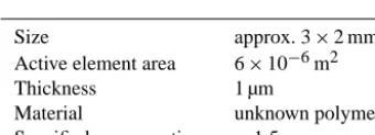
Table 1. Overview of P14 Rapid characteristics.

Size approx. 3×2 mm

Active element area 6×10−6m2

Thickness 1 µm

Material unknown polymer

Specified response time <1.5 s

In airborne measurements, a wide variety of customized instruments is being used, including, e.g., Lyman-α absorp-tion hygrometers (e.g. Buck, 1976; Bange et al., 2002), tun-able diode laser absorption spectroscopy hygrometers (TD-LAS, e.g. May, 1998; Zondlo et al., 2010; Paige, 2005), infrared absorption hygrometers (e.g. LI-7500A), chilled-mirror dew point instruments (DPM, Neininger et al., 2001), krypton hygrometers (Campbell et al., 1985; Thomas et al., 2012) or polymer-based thin-film capacitive absorption hy-grometers (see Spieß et al., 2007; Reuder et al., 2009). Only the optical instruments are usually used for turbulence anal-ysis.

Additional sensor types that have not previously been mentioned and are found in ground-based meteorology are psychrometers and resistive or inductive hygrometers. 2.2 Capacitive humidity sensors

None of the instruments that are used on manned aircraft can easily be carried by small RPA, where compact size and light weight are essential. A trade-off has to be made regarding ac-curacy, response time and long-term stability of the sensors. Considering all the sensor types mentioned in Sect. 2.1, only the capacitive humidity sensor can be easily integrated into a small RPA with current state of the art technology. The size of these elements is typically less than 1 cm2, and, in non-severe conditions, accuracy and stability of the elements is adequate.

Table 2. List of tested polymer-based humidity sensors

Model Company

P14 Rapid IST AG G-US.171R2 U.P.S.I. HIH4030 Honeywell HYT-241 Hygrosens SHT75 Sensirion

HMP50 Vaisala

DigiPicco IST AG HTM-B71 Tronsens

Capacitive humidity sensors are in most cases based on thin-film polymers (Tetelin and Pellet, 2006; Sen and Darabi, 2008; Shibata et al., 1996). The materials adsorb water at the sensor surface from where it diffuses into the material and changes the relative permittivity and therefore the capaci-tance of the sensor (see Sect. 2.3). With decreasing thickness of the polymer, the time constant also decreases. One of the fastest of this kind on the market is the P14 Rapid by Inno-vative Sensor Technology (IST) AG (Fig. 1, Table 1), which has a time response of<1.5 s falling edge, according to the specification (IST AG, 2009). Other sensors that are com-mercially available and were tested, both in a climate cham-ber and in flight, are listed in Table 2. The sensors HYT-241, HTM-B71, SHT75 and DigiPicco have a digital output that only allows low sampling rates. HIH4030 and HMP50 are analogue sensors. All of these sensors showed a slower time response than the P14 Rapid. The G-US.171R20 did show a very fast response to humidity changes but was extremely sensitive to temperature changes as well. The calibration of this sensor was not found to be stable in the long term.

(4)

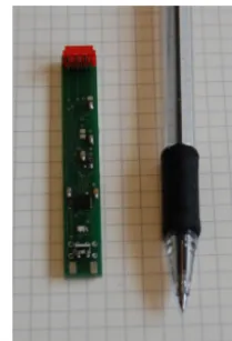
Figure 2. Humidity sensor on printed circuit board with the

capac-itance measurement chip PCAP01.

Applied Sciences Ostwestfalen-Lippe and the University of Tübingen. The computer stores the data at 100 Hz onto an SD card. At the same time, the sensor signal can be monitored in real time on a remote computer.

In order to better understand the measurements that are done with the P14 Rapid, Sect. 2.3 introduces a model which relates the measured capacitance to the water concentration in the polymer. In a steady state, the water concentration in the polymer equals the water concentration at the sensor surface. Section 2.4 introduces a calibration to get the rela-tive humidity from the surface water concentration. Finally, Sect. 3 describes how the diffusion process of water from the sensor surface into the polymer can be modelled and how, by inversion of this model, the surface concentration of the sensor – and thus the ambient relative humidity – can be es-timated throughout a measurement flight.

2.3 Physical model

In Sect. 3, a dynamical model will be presented, which de-scribes the change of water concentration in the polymer with time. In order to work with this model, it is necessary to translate the measurement variable capacitanceCto the cor-responding average water concentration in the polymerc. In this section, a physical model is presented, which describes this relation. In a parallel-plate capacitor, the charge per volt-age is defined as the capacitance. It can also be expressed as a function of the areaAof the parallel plate, the distanced

between the plates, the relative permittivityεrof the material between the plates and the vacuum permittivityε0:

C=Q

U =ε0εr A

d =(εr−1)ε0 A d +ε0

A

d. (1)

For the following investigation, it helps to decompose the capacity of the humidity sensor into partial capacities (Eq. 2), in particular the capacitance of the vacuum between the platesC0, the capacitance of the polymer aloneCPolyand the capacitance of absorbed water in the polymer CH2O.CPoly

andC0 are constant and provide an offset capacitance for zero water concentration, whileCH2Oaccounts for the

sensi-tivity of the capacitance to changes in water concentration in the polymer.

C=ε0(εHr2O+ε Poly r )

A d

=ε0εrPoly

A d

| {z }

:=CPoly

+(εH2O

r −1)ε0

A d

| {z }

:=C_H2O

+ε0

A d

|{z} :=C0

. (2)

The Debye equation for molar polarisationPm connects the microscopic characteristics, which are the electrical dipole momentµand the polarizabilityα, to the relative per-mittivityεrof a material (Debye, 1929).

Pm=

εH2O

r −1

εH2O

r +2 = Z

3ε0 ·

α+ µ

2

kBT

, (3)

with particle density Z= %

MNA and%being the density,M the molecular mass,NAthe Avogadro constant,kBthe

Boltz-mann constant andT the temperature.εH2O

r can be derived from Eq. (2) to yield

εH2O

r =

C−CPoly

C0

. (4)

The particle densityZcan also be expressed as the integral of water concentrationcin the volume

Z(t )= ˆ

z

ˆ

y

ˆ

x

c(x, y, z, t )dxdydz·NA

V . (5)

For spatially constant concentration (∇c=0)

Z=c·V·NA

V =c·NA . (6)

With the help of Eqs. (2), (3) and (6), water concentration can be found as a function of capacitance and temperature:

c=

(C−CPoly)

C0 −1

(C−CPoly)

C0 +2

· 3ε0

α+ µ2

kBT

· 1

NA

C−CPoly

C0 −1

2+C−CPoly

C0

· 1

QNA . (7)

WhileC is the capacitance actually measured andC0 is defined asε0A_d,Cpolyis unknown before calibration. It is es-timated by extrapolation of the calibration regression to zero relative humidity. The calibration procedure is described in Sect. 2.4.

2.4 Calibration

(5)

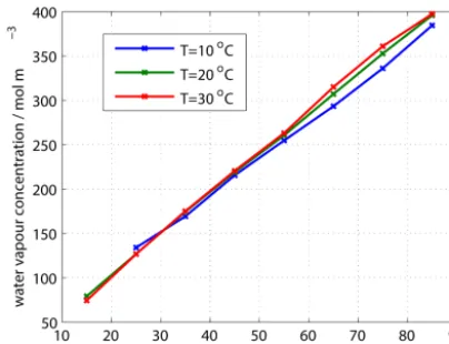
Figure 3. Calibration of a P14 Rapid humidity sensor. Calibration

was done at three different temperatures.

time. The dynamics of this process are modelled in Sect. 3. For the calibration, humidity is held at a constant level for at least 30 min to assure equilibrium of the water concen-tration. It is not necessarily the case that polymer-based ca-pacitive humidity sensors show a linear relationship between measured capacitance and relative humidity (Shibata et al., 1996). Figure 3 shows the result of three calibrations at three different temperatures. On theyaxis of the graph, the mea-sured capacitance was directly translated into water vapour concentration, according to Eq. (7). Before doing this,Cpoly must be set, so that an extrapolation of the curve in Fig. 3 will yield zero water concentration in the polymer at zero ambient relative humidity. A practical way to get a good es-timation forCpolyis to find the zero-crossing of a regression curve between measured capacitance and relative humidity, which is(Cpoly+C0). SinceC0is a known sensor property,

Cpoly can be calculated and was found to be approximately 60 pF for the sensor examined here. The temperature in the calibration chamber is kept constant and relative humidity is increased stepwise from 15 to 85 % during the calibration. A dew point mirror in conjunction with a PT100 tempera-ture sensor inside the calibration chamber is used as refer-ence instrument to control relative humidity and temperature. While sensor physics depends on both temperature and wa-ter vapour partial pressure, the P14 Rapid follows a linear relationship with relative humidity within the calibrated tem-perature range. The calibration chamber used was calibrated against a secondary standard with an accuracy of 0.4 % RH. A root mean square error of less than 1 % RH between the calibration curve and the measured values is found for the ca-pacitive humidity sensor calibration in the chamber at 10◦_C or more. The facilities that were available to the authors did not allow calibration at lower temperatures.

6 N. Wildmann et. al: Capacitive Humidity Sensor Inverse Modelling

               ∂c₁ ∂t ∂c2 ∂t ∂c₃ ∂t ∂c₄ ∂t .. . .. . ∂cN−1

∂t ∂cN ∂t                =               

−2Y Y 0 0 0 0 · · · 0

Y −2Y Y 0 0 0 · · · 0

0 Y −2Y Y 0 0 · · · 0

0 0 Y −2Y Y 0 · · · 0

..

. . .. ...

.

.. . .. ...

0 0 0 0 · · ·Y −2Y −Y

0 0 0 0 · · · 0 Y −Y

               ·                c1 c2 c3 c4 .. . . .. cN−1

cN                +                Y 0 0 0 .. . . .. 0 0               

·cs

cm= (1 1 1· · ·1)        c₁ N c₂ N c₃ N . .. cN N        (14) ∆x d · · · cs c1 c2 c3

cN−1

cN l l l l l l l l l l l l

Fig. 4. Sketch of the sensor model.

Boundary conditions exist for the layer at the surface of the sensor and the bottom most layer. At the surface layer the concentration that is adsorped from ambient water vapour diffuses into the layer. At the bottom, no diffusion is possible 380

from below.

Equation 14, translated to vector notation, conforms with the standard layout of a single-input-single-output (SISO) state-space model, as it is used in control theory (Lutz and Wendt, 2007):

385

∂

∂tc=Yc+ (Y 0 0· · ·0) T cs cm= 1 N 1 N 1 N · · ·

1 N

c (15)

The vector c of water concentrations in each layer of the model is the state vector. The diffusion matrix Y is the sys-390

tem (or state) matrix, which describes how the current con-centrations c in each layer affect the change in concon-centrations

∂

∂tc. The input (or control) vector(Y 0 0· · ·0) T

determines how the system input affects the states c. It is modelled to describe the diffusion of water vapour into the top most layer 395

of the sensor. The single input variable of the whole system is the surface concentrationcsand the single output variable is the averaged water concentration in the polymercm, that is presented as a function of the measured capacitance in

equa-0 5 10 15

55 60 65 70 75 80

time / s

rel. humidity / %

0 5 10 15

55 60 65 70 75 80

time / s

0 5 10 15

30 40 50 60

time / s

0 5 10 15

30 40 50 60

time / s

step

measured

modelled

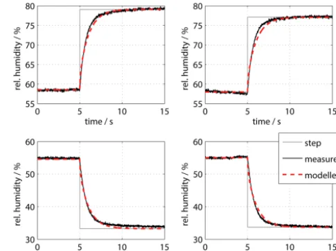
Fig. 5. Result of a step response experiment with rising edge (upper

figures) and falling edge (lower figures) humidity in comparison to model results. The model was run with 40 layers and a diffusion coefficientD= 0.38µm2

s−1_{in all cases.}

tion 7. The so-called output vector _N1 _N1 _N1 · · · 1

N

maps 400

the states c to the output variablecm, which in the case of the sensor model is a simple averaging of the concentrations in all layers.

Model validation

To show that this model does agree with reality, step response 405

experiments with rising and falling edge steps of humidity were performed. The results in figure 5 show that the model fits well with reality, if the correct diffusion coefficient is ap-plied. Of course, it has to be noted that the diffusion coef-ficient, since it is the one unknown parameter in the model, 410

also serves as a correction factor for other model inaccuracies and therefore is most likely not the true physical diffusion

co-Figure 4. Sketch of the sensor model.

3 Dynamic signal restoration 3.1 Dynamic model

A dynamic model describes the behaviour of a system over time. This behaviour is typically described mathematically by a set of differential equations. In the case of a capaci-tive humidity sensor, the dynamics are mainly influenced by the diffusion of water vapour from the sensor surface into the polymer. While the water concentrationcin the polymer was constant in space in the stationary model described in Sect. 2.3, the following section will describe how the con-centration changes in time and space. The diffusion flux J is described by Fick’s law as shown in Eq. (8). It is assumed that a model with a spatially constant diffusion coefficientD

describes the behaviour of the sensor well enough. Figure 4 shows a sketch of the model of finite volumes in the sensor polymer.

J= −D· ∇c (8)

Combined with the continuity equation of mass conserva-tion (Eq. 9), Fick’s second law can be derived (Eq. 10).

∂c

∂t = −∇ ·J (9)

=D∇2c (10)

Since these equations yield a differential equation of sec-ond order, a simplification is needed to find a manageable solution. A common solution to these kinds of problems is a numerical approach, such as the finite-volume method (LeV-eque, 2002). According to this method, the mass conserva-tion Eq. (9) is integrated over a finite-volume elementVn. ˚

Vn

∂c

∂t dV = −

˚

Vn

(∇ ·J)dV (11)

The divergence theorem (or the combination of the conti-nuity equation with the Gauss theorem) allows one to write the right-hand side of the equation as a surface integral. The left-hand side can be solved to obtain the product of spatially averaged concentration change in a volume element and its volume.

∂cn

∂t Vn= −

‹

s

(6)

In the following, concentrations with an index always rep-resent spatial averages over a finite volume, and the overbar notation to indicate the averaging, as incn, will be omitted. Concentration gradients in horizontal directions are consid-ered to be 0, as the sensor is small enough that a constant humidity above the whole sensor surface can be assumed. Therefore, there will be no horizontal fluxes of water and the volume elementsVncan be simplified to layers as shown in

Fig. 4. The surface integral can be simplified to the sum of diffusion from the layer above (n−1) and the layer below (n+1) for each layernin the polymer and therefore yields

∂cn

∂t =

−D·cn−cn−1

1x ·An,n−1

Vn

+

−D·cn−cn+1

1x ·An,n+1

Vn

, (13) where An,n−1 and An,n+1 are the top and bottom surface area of the polymer layers respectively and 1x is the layer thickness. A matrix representation of the simplified diffusion model with Y= D·A

1x·Vn is given in Eq. (14).              ∂c1 ∂t ∂c₂ ∂t ∂c₃ ∂t ∂c4 ∂t . . . . . .

∂cN−1 ∂t ∂cN ∂t              =         

−2Y Y 0 0 0 0 · · · 0 Y −2Y Y 0 0 0 · · · 0 0 Y −2Y Y 0 0 · · · 0 0 0 Y −2Y Y 0 · · · 0

. . . ._. . . . . . . . ._. . . . . 0 0 0 0 · · · Y −2Y −Y 0 0 0 0 · · · 0 Y −Y

         ·          c1 c2 c3 c4 . . . . . .

cN−1

cN          +          Y 0 0 0 . . . . . . 0 0         

·cs

cm=(1 1 1 · · ·1)        c1 N c2 N c3 N .. . cN N        (14)

Boundary conditions exist for the layer at the surface of the sensor and the bottommost layer. At the surface layer the concentration that is adsorbed from ambient water vapour diffuses into the layer. At the bottom, no diffusion is possible from below.

Equation (14), translated to vector notation, conforms with the standard layout of a single-input–single-output (SISO) state–space model as used in control theory (Lutz and Wendt, 2007):

∂

∂tc=Yc+(Y0 0· · · 0)

T_c

s

cm=

₁

N

1

N

1

N · · ·

1

N

c. (15)

Figure 5. Result of a step response experiment with rising-edge

(up-per figures) and falling-edge (lower figures) humidity in comparison to model results. The model was run with 40 layers and a diffusion coefficientD=0.38 µm2s−1in all cases.

The vectorc of water concentrations in each layer of the model is the state vector. The diffusion matrix Y is the system (or state) matrix, which describes how the current concentra-tionscin each layer affect the change in concentrations _∂t∂c. The input (or control) vector(Y 0 0· · ·0)T determines how the system input affects the statesc. It is modelled to describe the diffusion of water vapour into the topmost layer of the sensor. The single-input variable of the whole system is the surface concentrationcsand the single output variable is the averaged water concentration in the polymercmthat is pre-sented as a function of the measured capacitance in Eq.(7). The so-called output vector_N1 _N1 _N1 · · · 1

N

maps the states

cto the output variablecm, which, in the case of the sensor model, is a simple averaging of the concentrations in all lay-ers.

3.1.1 Model validation

(7)

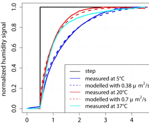
Figure 6. Step responses of the same sensor at different

tempera-tures. Theyaxis is normalized to 0 for humidity before the step and 1 for humidity after the step. This is legitimate since the dynamics does not depend on the step amplitude.

the sensor changes completely in less than 100 ms, based on the outlet flow of the generator and the size of the chamber. Comparing the rising and falling edge steps, it becomes evi-dent that no difference in time response can be observed for both cases, and the model works with the same diffusion co-efficient without hysteresis. This implies that diffusion is the dominant factor in comparison to adsorption and desorption regarding the dynamics of the sensor, and the model is suit-able for describing the dynamic behaviour of the sensor.

To investigate the sensitivity of the diffusion coefficient to ambient temperature, tests were done at three different temperatures (5, 20 and 37◦C). The result in Fig. 6 shows that the diffusion coefficient at 5◦C is lower compared to the other two temperatures, which agree quite well. This means that it is not possible to apply a universal diffusion coeffi-cient for one sensor, but the diffusion coefficoeffi-cient needs to be adapted to the given ambient temperature, especially in low-temperature environments. However, small deviations as they appear in the ABL will not be critical for the model. 3.2 Inverse model for signal restoration

Having found a model that reasonably describes the dynamic behaviour of the sensor, it is now possible to use this model to restore the original signal of relative humidity in the atmo-sphere from measured data. For this purpose it is necessary to invert the model, which is equivalent to solving the system equations for the surface water vapour concentrationcs.

Since the state–space model cannot easily be inverted, the first step is to transform Eq. (15) to a transfer function in the Laplace domain. This can be done as presented in Eq. (16)

according to Lutz and Wendt (2007).

cm(s)=

₁

N

1

N · · ·

1

N

(sE−Y)−1(Y 0 · · ·0)T · cs(s) =G(s)· cs(s) (16) E is a unity matrix of the same dimensions as the system ma-trix Y. The variables is a result of the Laplace transforma-tion.G(s)is the transfer function in the Laplace domain. A transfer function of a linear dynamic system can be expressed as a fraction with a numerator and a denominator polynomial of the parametersin the Laplace domain (Astrom and Mur-ray, 2009, chapter 8). This fraction can simply be inverted to solve Eq. (16) for the original signal:

cs(s)=G(s)−1· cm(s). (17)

A drawback of this method is that it only works well if the measured signal and the applied model fit well. Noise that is not modelled will be amplified more with increasing polynomial order in the transfer function. On the other hand, the model will be more accurate with a higher number of modelled layers in the polymer, which leads to a high poly-nomial order in the transfer function. A way of dealing with this problem is oversampling and careful filtering of the mea-sured signal in order to achieve a good signal-to-noise ratio.

Figure 7 shows a signal flow block diagram (see, e.g., Astrom and Murray, 2009, pp. 55–59) of the signal restora-tion. It includes input and output filters that were applied to achieve a restored signal that is not disturbed by amplified noise of the inverse modelling. For the input, a sharp low-pass filter of 20th order at a cutoff frequency of 10 Hz is cho-sen to eliminate the white noise of the capacitance measure-ment, which dominates above this frequency. In the output filter, a first-order low pass is good enough to filter out the remaining noise after the signal restoration. The block dia-gram was generated with Matlab Simulink®, which was also used in a first approach to carry out the convolution of the measured signal with the transfer function.

4 Results

4.1 Vertical profiles

(8)

Figure 7. Block diagram of signal restoration. The input signal of the humidity sensor is filtered with a Butterworth filter of order 20 at a

cutoff frequency of 10 Hz. After the inverse transformation, the signal is filtered again with a simple first-order delay low pass with cutoff frequency at 15 Hz.

Figure 8. Vertical profile of relative humidity before and after

cor-rection.

In Fig. 8, a vertical profile is shown with raw measure-ments and with a restored signal for relative humidity, ap-plying the method described in Sect. 3. It clearly shows how an offset present between ascent and descent of the flight is eliminated in almost every detail, except for a few altitudes, where obviously local events of water vapour disturb the con-tinuity of the profile, as can be seen between 150 and 200 m or at 350 m barometric altitude. The parameter that is critical to tune in the sensor model is the diffusion coefficient as de-scribed above. Within the minute or two that are needed for an ascent and a descent of a vertical profile with the RPA, in a nonconvective boundary layer, the mean relative humid-ity will not shift into one direction or the other, so that the parameter can be tuned to show a minimum offset between ascent and descent. Once the diffusion coefficient is found from a vertical profile, it is possible to use this parameter for the signal restoration of the complete flight with a duration of 30–60 min. It is, however, recommended to redo the vertical profile diffusion coefficient estimation for each flight since contamination and small damage invisible to the human eye were found to significantly change the sensor dynamics. Dif-ferent sensors of the same batch can even show slightly dif-ferent characteristics. Of course, this way of determining the diffusion coefficient only works if gradients of water vapour concentration do exist at least in parts of the vertical profile.

Figure 9. Power spectrum of relative humidity before and after

cor-rection. The number of layers in the sensor model is set toN=40. From the vertical profile, the diffusion constant was found to be

D=0.1 µm2s−1. The spectrum is averaged over five flight legs.

4.2 Spectral response

A MASC RPA at the University of Tübingen is equipped with fast sensors for temperature and wind measurement in order to measure turbulence. The goal of this study is to make turbulence studies for water vapour possible with capacitive humidity sensors. To quantify the improvements that were achieved in working towards this goal, it is useful to investi-gate the spectral response of the sensor before and after the signal restoration. Figure 9 shows the power spectral den-sity of the relative-humidity signal over the frequency for both cases. The original signal is strongly effected by the slow sensor dynamics for frequencies above 0.05 Hz (red curve). At about 3 Hz the signal vanishes in noise entirely (spectral power is almost constant for higher frequencies). The restored signal almost perfectly follows the expected −5/3 slope for locally isotropic turbulence in the inertial subrange according to Kolmogorov (1941), until about 3 Hz (blue curve). For higher frequencies, noise is dominant and thus is the limiting factor of the signal restoration.

(9)

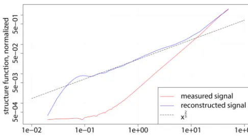
Figure 10. Structure function before and after correction.The

num-ber of layers in the sensor model is set toN=40. The diffusion constant was found to beD=0.1 µm2s−1from the vertical profile. The structure function is normalized by 2σ2and averaged over five flight legs.

indication of sensor dynamics or other errors in the measure-ment; this is the case even more clearly than for the power spectral densities. Figure 10 shows how close the structure function of the restored signal is to the theory until a time lag of about 0.3 s (corresponding to 3 Hz), especially compared to the original signal.

5 Conclusions

This report addressed the problem of water vapour measure-ment for turbulence analysis with small RPA. It was estab-lished that capacitive humidity sensors are currently the only feasible solution for these measurements onboard an RPA of 5 kg, as operated in Tübingen, or smaller. A method is intro-duced to enhance the quality of such measurements with the help of control theory methods in post-processing. The dy-namic diffusion model derived in Sect. 3 is therefore inverted to find the water concentration on the sensor surface from measured average water concentration in the polymer. Since the measurement variable of the sensor is, in the first place, the capacitance, the physics of how to translate the mea-sured capacitance into water concentration was introduced in Sect. 2.3. A calibration approach was used to connect sen-sor surface water concentration to ambient relative humidity (Sect. 2.4). To summarize, the model can be applied in five steps:

1. calculation of average water concentration in the poly-mer cm for a time series of capacitance of the sensor according to Sect. 2.3;

2. setup of the state–space model according to Sect. 3.1; 3. conversion of the state–space model into a transfer

func-tion according to Sect. 3.2, Eq. (16);

4. deconvolution of the measured average water concen-tration signalcmin the polymer with the transfer func-tion in order to find the water concentrafunc-tion at the sur-face of the polymercs(Eq. 17);

5. recovery of the relative humidity from the surface wa-ter concentrationcsthrough the calibration described in Sect. 2.4.

It is shown in Sect. 4 how vertical profiles can be corrected using the presented method. We propose using a minimiza-tion of error between ascent and descent of a vertical profile flight with an RPA to find the correct diffusion coefficient for the given temperature and sensor. This is necessary, since the exact relation between diffusion coefficient and temperature could not be determined in a laboratory experiment and infor-mation about the polymer type is not available. The benefit of determining the diffusion coefficient empirically for each measurement flight is that this parameter is the only unknown in the dynamic model and therefore can also be used to cor-rect for other inaccuracies in the model. A spectral analy-sis of flight legs in the atmospheric boundary layer with a diffusion coefficient determined from a vertical profile dur-ing the same flight showed promisdur-ing results for turbulence analysis. It can be stated that the enhancement of the sen-sor makes it possible to resolve turbulent fluctuations up to 3 Hz, which corresponds to a 10 m eddy size at 25 m s−1 air-speed. Compared to temperature and wind measurement on a MASC RPA (up to 20 Hz), this is still fairly low and will need to be improved in future work. The main constraints for the given setup are the signal-to-noise ratio and the sensitivity of the capacitance measurement. Improvements of the measure-ment circuit with several parallel sensors can possibly solve this problem. Measurements of turbulent fluctuations up to 10 Hz seem possible. The systematic approach of the signal restoration is open to further extensions of the sensor model, e.g. physical descriptions of water adsorption on the sensor surface or temperature dependence of diffusion into the poly-mer. These extensions can lead to significantly higher com-plexity, which cannot be described by a linear time-invariant system any more. For measurements in the summer convec-tive boundary layer in central Europe, the described simpli-fications are appropriate and provide promising results. To apply the method in very cold temperatures or in radiosonde applications, where strong temperature differences are expe-rienced in a single ascent, further studies that are beyond of the scope of this paper are required.

Acknowledgements. We are grateful to one anonymous referee and the Associated Editor Murray Hamilton for their fruitful comments, which helped to improve the quality of this paper.

(10)

We acknowledge support by the Deutsche Forschungsge-meinschaft and the Open Access Publishing Fund of Tübingen University.

Edited by: M. Hamilton

References

Astrom, K. and Murray, R.: Feedback Systems: An Introduction for Scientists and Engineers, Princeton University Press, 2009. Bange, J. and Roth, R.: Helicopter-Borne Flux Measurements in the

Nocturnal Boundary Layer Over Land – a Case Study, Bound.-Lay. Meteorol., 92, 295–325, 1999.

Bange, J., Beyrich, F., and Engelbart, D. A. M.: Airborne Measure-ments of Turbulent Fluxes during LITFASS-98: A Case Study about Method and Significance, Theor. Appl. Climatol., 73, 35– 51, 2002.

Bange, J., Esposito, M., and Lenschow, D. H.: Airborne Measure-ments for Environmental Research – Methods and InstruMeasure-ments, chap. 2: Measurement of Aircraft State, Thermodynamic and Dy-namic Variables, 641 pp., Wiley, 2013.

Buck, A. L.: The Variable-Path Lyman-Alpha Hygrometer and Its Operating Characteristics, Bull. Am. Meteorol. Soc., 57, 1113– 1118, 1976.

Campbell, G., Tanner, B., and Gauthier, R.: Krypton hygrometer, available at: http://www.google.com/patents/US4526034 (last access: 17 September 2014), uS Patent 4,526,034, 1985. Chao, H., Baumann, M., Jensen, A., Chen, Y., Cao, Y., Ren, W., and

McKee, M.: Band-reconfigurable multi-UAV-based cooperative remote sensing for real-time water management and distributed irrigation control, IFAC World Congress, Seoul, Korea, 2008. Corsmeier, U., Hankers, R., and Wieser, A.: Airborne Turbulence

Measurements in the Lower Troposphere Onboard the Research Aircraft Dornier 128-6, D-IBUF, Meteorol. Z., 4, 315–329, 2001. Debye, P.: Polare Molekeln, S. Hirzel, Leipzig, 200 pp., 1929. Eckles, R.: Gas analyzer, available at: http://www.google.com/

patents/US6317212 (last access: 17 September 2014), uS Patent 6,317,212, 2001.

Garratt, J.: The Atmospheric Boundary Layer, University Press, Cambridge, 1992.

IST AG: P14 – Rapid Capacitive Humidity Sensor, datasheet V4.3-11/2009, 2009.

Jensen, A. and Chen, Y.: Tracking tagged fish with swarming un-manned aerial vehicles using fractional order potential fields and Kalman filtering, in: 2013 International Conference on Un-manned Aircraft Systems (ICUAS), 1144–1149, IEEE, 2013. Jonassen, M. O.: The Small Unmanned Meteorological Observer

(SUMO), Master’s thesis, University of Bergen – Geophysical Institute, 2008.

Kolmogorov, A.: The Local Structure of Turbulence in Incompress-ible Viscous Fluid for Very Large Reynolds Numbers, Dokl. Akad. Nauk SSSR, 30, 299–303, reprint: Proc. R. Soc. Lond. A, 1991, 434, 9–13, 1941.

Kuisma, H., Lehto, A., and Jalava, J.: Capacitive humidity sen-sor and method for the manufacture of same, available at: http: //www.google.com/patents/US4500940 (last access: 17 Septem-ber 2014), uS Patent 4,500,940, 1985.

Leiterer, U., Dier, H., Nagel, D., Naebert, T., Althausen, D., Franke, K., Kats, A., and Wagner, F.: Correction Method for RS80-A

Hu-micap Humidity Profiles and Their Validation by Lidar Backscat-tering Profiles in Tropical Cirrus Clouds, J. Atmos. Oceanic Technol., 22, 18–29, 2005.

LeVeque, R. J.: Finite Volume Methods for Hyperbolic Problems, Cambridge University Press, doi:10.1017/CBO9780511791253, 2002.

Lutz, H. and Wendt, W.: Taschenbuch der Regelungstechnik: mit MATLAB und Simulink, Harri Deutsch, Frankfurt am Main, Germany, 2007.

Maronga, B.: Monin-Obukhov similarity functions for the structure parameters of temperature and humidity in the unstable surface layer: results from high-resolution large-eddy simulations, J. At-mos. Sci., 71, 716–733, doi:10.1175/JAS-D-13-0135.1, 2013. Martin, S. and Bange, J.: The Influence of Aircraft Speed

Variations on Sensible Heat Flux Measurements by Differ-ent Airborne Systems, Bound.-Lay. Meteorol., 150, 153–166, doi:10.1007/s10546-013-9853-7, 2013.

Martin, S., Bange, J., and Beyrich, F.: Meteorological profiling of the lower troposphere using the research UAV “M2AV Carolo”, Atmos. Meas. Tech., 4, 705–716, doi:10.5194/amt-4-705-2011, 2011.

Martin, S., Beyrich, F., and Bange, J.: Observing Entrain-ment Processes Using a Small Unmanned Aerial Vehicle: A Feasibility Study, Bound.-Lay. Meteorol., 150, 449–467, doi:10.1007/s10546-013-9880-4, 2013.

May, R. D.: Open-path, near-infrared tunable diode laser spectrom-eter for atmospheric measurements of H2O, J. Geophys.

Res.-Atmos., 103, 19161–19172, doi:10.1029/98JD01678, 1998. Miloshevich, L. M., Paukkunen, A., Vömel, H., and Oltmans,

S. J.: Development and Validation of a Time-Lag Correction for Vaisala Radiosonde Humidity Measurements, J. Atmos. Oceanic Technol., 21, 1305–1327, doi:10.1175/jtech1770.1, 2004. Neininger, B., Fuchs, W., Baeumle, M., Volz-Thomas, A., Prévôt,

A. S. H., and Dommen, J.: A Small Aircraft for More Than Just Ozone: MetAir’s ’Dimona’ After Ten Years of Evolving Devel-opment, in: 11th Symp. on Meteorological Observations and In-strumentation, Albuquerque, NM, Amer. Meteor. Soc., 123–128, 2001.

Paige, M. E.: Compact and Low-Power Diode Laser Hygrometer for Weather Balloons, J. Atmos. Oceanic Technol., 22, 1219–1224, doi:10.1175/jtech1770.1, 2005.

Rediniotis, O. and Pathak, M.: Simple Technique for Frequency-Response Enhancement of Miniature Pressure Probes, AIAA Journal, 37, 897–899, 1999.

Reuder, J., Brisset, P., Jonassen, M., Müller, M., and Mayer, S.: The Small Unmanned Meteorological Observer SUMO: A new tool for atmospheric boundary layer research, Meteorol. Z., 18, 141– 147, 2009.

Sen, A. and Darabi, J.: Modeling and Optimization of a Microscale Capacitive Humidity Sensor for HVAC Applications, Sensors Journal, IEEE, 8, 333–340, 2008.

Shibata, H., Ito, M., Asakursa, M., and Watanabe, K.: A digital hy-grometer using a polyimide film relative humidity sensor, IEEE Trans. Instr. Measure., 45, 564–569, 1996.

Spieß, T., Bange, J., Buschmann, M., and Vörsmann, P.: First Ap-plication of the Meteorological Mini-UAV “M2AV”, Meteorol. Z. N. F., 16, 159–169, 2007.

(11)

Tagawa, M., Kato, K., and Ohta, Y.: Response compensation of fine-wire temperature sensors, Rev. Sci. Instrum., 76, 094904, 4 pp., 2005.

Tetelin, A. and Pellet, C.: Modeling and optimization of a fast re-sponse capacitive humidity sensor, Sensors Journal, IEEE, 6, 714–720, 2006.

Thomas, R. M., Lehmann, K., Nguyen, H., Jackson, D. L., Wolfe, D., and Ramanathan, V.: Measurement of turbulent water va-por fluxes using a lightweight unmanned aerial vehicle system, Atmos. Meas. Tech., 5, 243–257, doi:10.5194/amt-5-243-2012, 2012.

van den Kroonenberg, A., Martin, S., Beyrich, F., and Bange, J.: Spatially-averaged temperature structure parameter over a het-erogeneous surface measured by an unmanned aerial vehicle, Bound.-Lay. Meteorol., 142, 55–77, 2011.

van den Kroonenberg, A. C., Martin, T., Buschmann, M., Bange, J., and Vörsmann, P.: Measuring the Wind Vector Using the Au-tonomous Mini Aerial Vehicle M2AV, J. Atmos. Oceanic Tech-nol., 25, 1969–1982, 2008.

Wildmann, N., Mauz, M., and Bange, J.: Two fast temperature sen-sors for probing of the atmospheric boundary layer using small remotely piloted aircraft (RPA), Atmos. Meas. Tech., 6, 2101– 2113, doi:10.5194/amt-6-2101-2013, 2013.

Wildmann, N., Ravi, S., and Bange, J.: Towards higher accuracy and better frequency response with standard multi-hole probes in tur-bulence measurement with remotely piloted aircraft (RPA), At-mos. Meas. Tech., 7, 1027–1041, doi:10.5194/amt-7-1027-2014, 2014.

Wyngaard, J. C. and Clifford, S. F.: Estimating Momentum, Heat, and Moisture Fluxes from Structure Parameters, J. Atmos. Sci., 35, 1204–1211, 1978.