www.atmos-meas-tech.net/7/3497/2014/ doi:10.5194/amt-7-3497-2014
© Author(s) 2014. CC Attribution 3.0 License.
Effect of surface BRDF of various land cover types on geostationary
observations of tropospheric NO
2
K. Noguchi1, A. Richter2, V. Rozanov2, A. Rozanov2, J. P. Burrows2, H. Irie3, and K. Kita4
1Faculty of Science, Nara Women’s University, Nara, Japan
2Institute of Environmental Physics, University of Bremen, Bremen, Germany 3Center for Environmental Remote Sensing, Chiba University, Chiba, Japan 4Faculty of Science, Ibaraki University, Mito, Japan
Correspondence to: K. Noguchi ([email protected])
Received: 30 January 2014 – Published in Atmos. Meas. Tech. Discuss.: 7 April 2014 Revised: 27 August 2014 – Accepted: 10 September 2014 – Published: 10 October 2014
Abstract. We investigated the effect of surface reflectance
anisotropy, bidirectional reflectance distribution function (BRDF), on satellite retrievals of tropospheric NO2. We
assume the geometry of geostationary measurements over Tokyo, which is one of the worst air-polluted regions in East Asia. We calculated air mass factors (AMF) and box AMFs (BAMF) for tropospheric NO2to evaluate the effect of
BRDF by using the radiative transfer model SCIATRAN. To model the BRDF effect, we utilized the Moderate Resolution Imaging Spectroradiometer (MODIS) products (MOD43B1 and MOD43B2), which provide three coefficients to express the RossThick–LiSparse reciprocal model, a semi-empirical and kernel-based model of BRDF. Because BRDF depends on the land cover type, we also utilized the High Resolu-tion Land-Use and Land-Cover Map of the Advanced Land Observing Satellite (ALOS)/Advanced Visible and Near In-frared Radiometer type 2 (AVNIR-2), which classifies the ground pixels over Tokyo into six main types: water, urban, paddy, crop, deciduous forest, and evergreen forest. We first develop an empirical model of the three BRDF coefficients for each land cover type over Tokyo and then apply the model to the calculation of land-cover-type-dependent AMFs and BAMFs. Results show that the variability of AMF among the land types is up to several tens of percent, and if we ne-glect the reflectance anisotropy, the difference with AMFs based on BRDF reaches 10 % or more. The evaluation of the BAMFs calculated shows that not considering BRDF will cause large errors if the concentration of NO2is high close
to the surface, although the importance of BRDF for AMFs decreases for large aerosol optical depth (AOD).
1 Introduction
Nitrogen dioxide (NO2) plays an important role in
tro-pospheric chemistry, and has been measured from space since the late 1990s. The spaceborne measurements from the Global Ozone Monitoring Experiment (GOME) (Burrows et al., 1999) and the Scanning Imaging Absorption Spectrom-eter for Atmospheric Cartography (SCIAMACHY) (Bovens-mann et al., 1999) successfully provided the horizontal dis-tributions of several tropospheric minor constituents includ-ing NO2. The GOME and SCIAMACHY instruments have
spatial resolutions of 40 km×320 km and 30 km×60 km, respectively. Improved spatial resolution of 13 km×24 km (nadir mode) is achieved with the Ozone Monitoring In-strument (OMI) onboard the Earth Observing System Aura, launched in 2004 (Levelt et al., 2006), followed by GOME-2 with a resolution of 40 km×80 km (Callies et al., 2000).
In previous studies, it was shown that measurements at such a high spatial resolution need more realistic parame-ters such as surface pressure, surface albedo, and reflectivity to derive accurate tropospheric NO2vertical column
densi-ties (VCDs) (Zhou et al., 2009; Boersma et al., 2011; Heckel et al., 2011; Russell et al., 2011). The authors indicated that the error from surface albedo was especially large. For ex-ample, Heckel et al. (2011) showed that the spread of NO2
air mass factor (AMF) values over land in a typical coastal area (around San Francisco) increases by±30 % on average if they used the surface albedo with high spatial resolution instead of coarse albedo which had been utilized in the previ-ous retrievals. Russell et al. (2011) showed that using surface
reflectance with a high resolution in NO2 retrievals
dimin-ished a false enhancement of NO2which were retrieved with
a coarse surface albedo over an unpolluted region. The re-duction of NO2amounts was up to 30 %.
One of the difficulties of treating surface albedo is its complex dependence on the incidence and outgoing direc-tions of light, which is expressed as the bidirectional re-flectance distribution function (BRDF). Because the pre-cise observations of BRDF for the entire global surface are difficult, nearly all previous studies assumed a Lambertian equivalent reflectivity (LER) surface for the operational re-trieval of the NO2 products. However, Zhou et al. (2010)
pointed out the importance of BRDF for tropospheric NO2
retrievals from OMI measurements, where viewing zenith angles on the ground surface are 0–70◦and the overpass time is 13:45 LT at the equator, showing that the differences be-tween the tropospheric NO2 VCDs using LER and BRDF
are 0–20 %. In their study, viewing angles largely changed with relatively constant solar zenith angles as OMI is aboard a sun-synchronous satellite. Lin et al. (2013) accounts for the BRDF effect in the retrievals of the tropospheric NO2
col-umn density over China using OMI measurements, and the authors showed that without consideration of the BRDF in the NO2 retrievals (OMI-based LER product was used for
the surface albedo), the tropospheric NO2VCDs decrease by
7 % on average with a variability of up to−45 % for individ-ual grid pixels compared to the retrievals with BRDF.
In the present study, we discuss the effect of BRDF on tropospheric NO2retrievals in future geostationary
measure-ments from the Geostationary Mission for Meteorology and Air Pollution (GMAP-Asia) in Japan (Akimoto et al., 2008, 2009), where a horizontal resolution of 10 km×10 km or less is planned. The GMAP-Asia aims to monitor air pol-lution in Asia, and the present study focuses on the Tokyo region (the Kanto Plain), which is one of the most polluted regions in Asia. Discussion of the effect of BRDF on geo-stationary measurements is also important since solar zenith angles and azimuth angles change largely throughout the day in geostationary measurements, much more so than for low earth orbits. The effect of BRDF can be critical, particularly if the diurnal variation of a tropospheric species is to be de-termined. The nature of BRDF of a given surface is largely dependent on the land cover type. Therefore, we first develop an empirical model of BRDF with consideration of various land cover types in the Tokyo area, and then apply the model to the evaluation of the BRDF effect on tropospheric NO2
retrievals.
2 Method
2.1 BRDF data
Following the method proposed by Zhou et al. (2010), we utilized the BRDF products derived from Moderate
Reso-Fig. 1. Definition of geometry angles of BRDF.
18
Figure 1. Definition of geometry angles of BRDF.
lution Imaging Spectroradiometer (MODIS) measurements (Justice et al., 1998). MODIS is aboard the Terra (EOS AM) and Aqua (EOS PM) satellites, and has six spectral bands in the wavelength region from 400 nm to 14.4 µm with spatial resolutions of 250, 500 and 1000 m, depending on the bands. In the present study, we utilized the channel 3 (459–479 nm) data.
The MODIS BRDF products adopted the RossThick– LiSparse reciprocal model, which is a semi-empirical and kernel-based model of BRDF (Lucht et al., 2000). The kernel components include the isotropic reflection effect, the vol-ume scattering effect, and the surface scattering and geomet-ric shadow casting effect:
BRDF(θ0, θ, φ, λ)=(1/ π ){fiso(λ)+fvol(λ) (1)
Kvol(θ0, θ, φ)+fgeo(λ)Kgeo(θ0, θ, φ)},
where θ0 is the solar zenith angle (SZA), θ is the
view-ing angle from the satellite,φis the relative azimuth angle, λis the wavelength, andKvol andKgeo are the volumetric
(RossThick) and geometric scattering (LiSparse-R) kernels, respectively (Roujean et al., 1992). This BRDF definition separates the dependence of BRDF on wavelength and the solar zenith and viewing angles. The definition of the three angles of the geometry, θ0, θ, and φ, is explained in
de-tail in Fig. 1. The three coefficients,fiso,fvol, andfgeo, are
determined from MODIS observations. The first coefficient, fiso, represents the component of non-directional reflectance
while other two coefficients,fvol andfgeo, are related with
the directional components of the surface reflectance. The details of these coefficients are described in Roujean et al. (1992) and Zhou et al. (2010). The spatial distributions of fiso,fvol, and fgeo over the Tokyo area were analyzed by
Noguchi et al. (2012).
Table 1. Definition of surface albedo types used in the present study.
Albedo type Reflectance nomenclature of Definition and implementation
Nicodemus et al. (1977) in the present study
BRF (bidirectional reflectance factors) BRF Angle dependence (θ0, θ, φ) is fully
considered, but treated as Lambertian equivalent reflectivity (LER) in RTM
BSA Directional hemispheric reflectance Integral of the BRDF over all viewing
(black-sky albedo) geometries. Only SZA dependence is considered,
and treated as LER in RTM
WSA Bihemispherical reflectance No consideration of angle
(white-sky albedo) dependence, and treated as LER in RTM
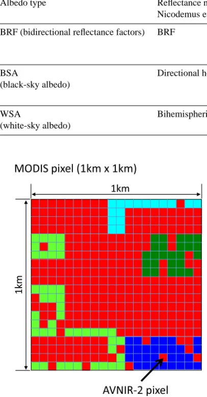
Fig. 2. Schematic of the MODIS and AVNIR-2 pixel sizes. For example, the dominance of the land cover
type shown in red for the MODIS pixel is calculated by dividing the number of the pixels in red (=285) by the number of all the pixels (=400).
19
Figure 2. Schematic of the MODIS and AVNIR-2 pixel sizes. For example, the dominance of the land cover type shown in red for the MODIS pixel is calculated by dividing the number of the pixels in
red (=285) by the number of all the pixels (=400).
mass factor (BAMF) of the tropospheric NO2. Table 1
ex-plains the differences among the approximations used. We calculated AMF and BAMF not only for BRDF but also for bidirectional reflectance factors (BRF), black-sky albedo (BSA), and white-sky albedo (WSA) to compare with the results among those definitions. In the reflectance nomen-clature of Nicodemus et al. (1977), BSA and WSA are so called directional hemispheric reflectance and bihemispher-ical reflectance, respectively. The three BRDF parameters, fiso,fvol, andfgeo, are included in the MODIS BRDF
prod-uct, MOD43B1 (Schaaf et al., 2002). We use the product MOD43B2 for a check of the data quality. The spatial reso-lution of the three BRDF parameters which we utilized in the
present study is 1 km×1 km. The values of BRF, BSA, and WSA are calculated for a given geometry based on MODIS parameters. Lucht et al. (2000) proposed and Zhou et al. (2010) also utilized a very good and simple approximation with a third-degree polynomial to calculate the numerical in-tegral ofKvolandKgeowith respect toθandφ:
BSA(θ0, λ)=fiso(λ)+fvol(λ)(−0.007574 (2) −0.070987θ02+0.307588θ03)+fgeo(λ)(−1.284909 −0.166314θ02+0.041840θ03).
In a similar way, Lucht et al. (2000) gave the values of the numerical integral ofKvol andKgeo with respect to all the
angles (θ0,θ, andφ):
WSA(λ)=fiso(λ)+0.189184fvol(λ)−1.377622fgeo(λ). (3) In the subsequent radiative transfer model (RTM), these fixed values are implemented as LER. This means that the BRF, WSA, and BSA are all treated as LER values when the AMF and BAMFs are calculated with the RTM. As for BRDF, the RTM directly reads the three parameters and then calculates AMF and BAMF considering the BRDF effect.
2.2 Land cover type data
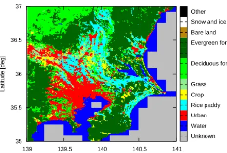
To take into account land cover types in the calculation of BRDF and other albedo types, we utilized the High Res-olution Land-Use and Land-Cover Map of Advanced Land Observing Satellite (ALOS)/Advanced Visible and Near In-frared Radiometer type 2 (AVNIR-2) (Fukue et al., 1997). The spatial resolution of the data set is approximately 50 m×50 m. As the grid size of AVNIR-2 is much smaller than that of MODIS, one MODIS grid pixel includes 400 pixels of AVNIR-2 (Fig. 2). Since there are few MODIS pix-els which consist of only one land cover type, we define the most frequent land cover type within each MODIS grid pixel as the representative land cover type of the pixel. Figure 3 shows the most dominant land cover type for each MODIS grid pixel over Tokyo. The land cover types which we focus on in the present study are summarized in Table 2.
139 139.5 140 140.5 141 Longitude [deg]
35 35.5 36 36.5 37
Latitude [deg]
Unknown Water Urban Rice paddy Crop Grass Deciduous forest Evergreen forest Bare land Snow and ice Other
Fig. 3. Land cover type map over the Kanto plain derived by AVNIR-2. The grid size is changed to a 1km square, which is the MODIS pixel size, from the AVNIR-2 original size of a 50msquare.
20
Figure 3. Land cover type map over the Kanto Plain derived from AVNIR-2. The grid size is changed to a 1 km square, which is the MODIS pixel size, from the AVNIR-2 original size of a 50 m square.
2.3 Atmospheric and geometric scenarios for
calculation of AMFs and BAMFs with SCIATRAN
We calculated the AMFs and BAMFs of the tropospheric NO2 with the RTM SCIATRAN (version 3.1.29), which
was developed to perform radiative transfer modeling for the purpose of the measurements of the earth’s atmosphere (Rozanov et al., 2005, 2014). SCIATRAN can perform radia-tive transfer calculations properly accounting for the spheri-cal shape of the earth’s atmosphere including refraction. In this study, the discrete-ordinates method, which is one of the options provided by SCIATRAN, was selected to solve the integro-differential radiative transfer equation in pseudo-spherical mode.
For the simulations, appropriate atmospheric and geomet-ric scenarios need to be defined. We defined 143 atmosphegeomet-ric layers between the altitudes of 0 and 100 km with a verti-cal resolution of 200 m (0–10 km), 500 m (10–12 km), and 1 km (12–100 km). We used a fixed NO2vertical profile
with-out seasonal or local time changes (Fig. 4). The scientific requirement team of the GMAP-Asia project provided this NO2profile data, which is based on the measurements
con-ducted by the TRACE-P aircraft mission (Jacob et al., 2003) and numerical simulations of the WRF-Chem model version 3.0.1 (Grell et al., 2005) with the conditions defined in Taki-gawa et al. (2007) and also in the CHASER model (Sudo et al., 2002). Pressure and temperature were taken from the US standard atmosphere 1976 (the average of midlatitudes). As for aerosols, we adopted a typical mixing state for ur-ban aerosols described in Hess et al. (1998) with the options prepared by SCIATRAN, following Noguchi et al. (2011). Table 3 summarizes the details of the aerosol conditions as-sumed in the present study. We also assume a vertical profile of the extinction coefficient with a scale height of 3 km and
Table 2. Land cover type and its identification number (ID) in the AVNIR-2 data set.
Land cover type ID
Water 1
Urban 2
Paddy 3
Crop 4
Deciduous forest 6
Evergreen forest 8
an aerosol optical depth (AOD) of 0.2 and 1.0 for comparison at a wavelength of 550 nm.
For the definition of the geometric scenario in SCIA-TRAN, three angles are needed; the SZA, the viewing angle from the satellite, and the relative azimuth angle (the angle between the sun and the satellite or an observation point at the ground surface). The definitions of those angles in SCI-ATRAN are depicted in Noguchi et al. (2011). We prepared a diurnal variation of SZAs and relative azimuth angles for summer and winter solstices as shown in Table 3 in Noguchi et al. (2011). The viewing angle at the surface is constant (46.4◦) for a geostationary satellite, which is chosen to be lo-cated at the altitude of 36 000 km over 120◦E on the equator.
3 Results
3.1 Empirical model of BRDF parameters
(fiso, fvol, fgeo) specific to land cover types
To obtain an empirical model of the typical BRDF param-eters for each land cover type over Tokyo, we computed monthly averages of the BRDF parameters,fiso, fvol, and
fgeo, grouped by MODIS pixels having the same land cover
type. As is described in Sect. 2.2, we classify each MODIS pixel to have one specific land cover type, which is the most dominant land cover type in the MODIS pixel. To select typ-ical MODIS pixels which represent each land cover type, we defined a threshold for the percentage of the most frequent AVNIR-2 land cover type in a MODIS pixel. As a sensitiv-ity study, the values offiso, fvol, andfgeo were compared
for different values of the land cover threshold (90, 95, and 100 %). Different values were used for crop land cover type (60 %), owing to the small number of MODIS pixels with a high ratio dominance of crop. Then, we created monthly averages of the three BRDF parameters for each land cover type. For example, we averaged all of the BRDF parameters, fiso,fvol, andfgeo, using only those MODIS pixels which
include 95 % or more of the “water” type of AVNIR-2 pixels to obtain the monthly mean BRDF parameters of the water type for the threshold of 95 %.
(a) (b)
0 2 4 6 8 10
0.01 0.1 1 10
Altitude [km]
NO2 VMR [ppbv]
0 2 4 6 8 10
1012 1013 1014 1015 1016
Altitude [km]
NO2 partial column density [cm -2
]
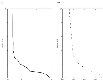
Fig. 4. Vertical profiles of (a)NO2volume mixing ratio (VMR) and (b)NO2partial column density of each
layer. Tropospheric (0–10km) total column density is 1.1×10¹⁶[cm−2].
21
Figure 4. Vertical profiles of (a) NO2volume mixing ratio (VMR) and (b) NO2partial column density of each layer. Tropospheric (0–10 km)
total column density is 1.1×10¹⁶[cm−2].
Table 3. Aerosol scenario.
Layer no. Altitude range Aerosol types Components and number Relative
mixing ratios humidity
#1 0–2 km Urban water soluble: 0.177 80 %
insoluble: 0.949×10⁻⁵
soot: 0.823
#2 2–10 km Continental average water soluble: 0.458 70 %
insoluble: 0.261×10⁻⁴
soot: 0.542
#3 10–30 km Sulfate sulfate: 1 0 %
#4 30–100 km Meteoric meteoric dust: 1 0 %
forest, and evergreen forest do not vary much if the thresh-old is increased from 90 to 100 % (see the Supplement). For the urban and rice paddy types, however, the results for 90 and 95 % are similar, but that for 100 % is different from the others. This is because the number of the pixels for 100 % is very small, only 20 pixels out of a total of 4248 urban-type pixels and just one pixel for a total of 3418 rice-paddy-type pixels.
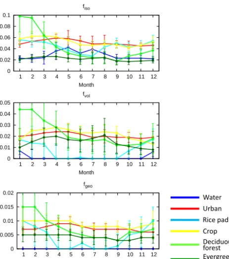
Therefore we decided to take a threshold percentage of 95 % land cover type dominance to obtain an empirical model of monthly averages of the BRDF parameters, fiso,
fvol, andfgeo, except for crop, for which we took a threshold
of 70 %. Figure 5 shows the results. We can see that the ur-ban type, which is a major land cover type in the polluted re-gion, has small seasonal dependence. This is consistent with the fact that urban surface features (e.g., buildings and roads)
are basically permanent, although plants beside roads and in parks possibly bring about some seasonality.
Deciduous and evergreen forests have a contrastive sea-sonality; the BRDF parameters of the deciduous forest type largely depend on season, but the evergreen forest type has a relatively small seasonality. The difference is caused by winter leaf drop in deciduous forests. As for the variability of the BRDF parameters (i.e., the magnitude of error bars), the land types covered with plants tend to have larger mag-nitudes than those of urban regions. If we strictly remove the pixels covered by plants from the urban region’s pixels, it may decrease the uncertainties related to BRDF’s seasonal-ity.
Here we focus on the seasonal change of rice paddies; rice paddies are distributed broadly in plain regions in Japan and also around Tokyo (see Fig. 3). Thefgeoandfvolof the rice
0 0.02 0.04 0.06 0.08 0.1
1 2 3 4 5 6 7 8 9 10 11 12 Month
fiso
0 0.01 0.02 0.03 0.04 0.05
1 2 3 4 5 6 7 8 9 10 11 12 Month
fvol
0 0.005 0.01 0.015 0.02
1 2 3 4 5 6 7 8 9 10 11 12 Month
fgeo
Fig. 5. Monthly averages of the MODIS BRDF parameters,fiso,fvolandfgeofor water (blue), urban (red), rice
paddy (light blue), crop (yellow), deciduous forest (light green) and evergreen forest (green). The land cover
type is derived by AVNIR-2.
22
Figure 5. Monthly averages of the MODIS BRDF parameters,fiso,
fvol, andfgeofor water (blue), urban (red), rice paddy (light blue),
crop (yellow), deciduous forest (light green), and evergreen forest (green). The land cover type is derived from AVNIR-2.
paddy type changes abruptly to close to zero in summer. This is caused by the nature of the water type, which has almost zero values throughout the year for bothfvolandfgeo, which
represent directional components of BRDF. This means that the water type has a small directional dependence of scat-tering (except for sun glint reflection). The seasonal change of rice paddies is caused by water cover in summer, while in other seasons no water exists in rice paddies. We should note such an abrupt change of the BRDF characteristics dur-ing that season in areas covered by rice paddies which often surround urban regions in Japan.
3.2 Tropospheric NO2AMFs including the BRDF effect
for each land cover type
Tropospheric NO2 AMFs for the BRDF surface are
calcu-lated for each land type (Fig. 6). The results show that the AMFs largely depend on land cover type, and the order of the AMFs’ magnitude between the different land cover types depends on season; in summer the AMF over urban sur-faces is largest, while in winter the rice paddy areas have the largest AMF. The AMF of evergreen forest is smallest both in summer and winter. The difference between the largest and smallest AMF is up to several tens of percent or even a factor of two. The variability among the land cover types is larger in summer than in winter and stronger at noon than in the morning or evening, which suggests that the dependence
of BRDF on land cover types becomes significant when the SZA is small.
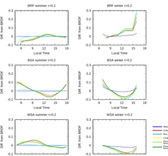
Figure 7 shows the relative difference of the AMFs for calculations using approximated surface types,ABRF,ABSA,
andAWSA, from the AMF for full BRDF treatment,ABRDF.
The difference depends in a complex way on season and lo-cal time differences fromABRDF being as large as 10 % or
more. With the exception of water and paddy surfaces, all land types show a similar behavior, indicating that the differ-ences are mainly in their total reflectivity and not the angular distribution. For the water-covered surfaces, the differences fromABRDF are generally small. In summer, the difference
is zero since thefvol andfgeo of water are zero. The AMF
of rice paddies in summer also has a small difference from ABRDF, which is similar to water since it is filled by water
during this season as discussed in Sect. 3.1. This means that ABRDFof rice paddies largely depends on season. The
dif-ference from the pure water type could be attributed to the non-water-covered regions of rice paddies, such as footpaths between rice fields.
The diurnal variations seen in Fig. 7 are a combination of changes in the AMF from the particular approximation used and changes in the AMF based on full BRDF calculations. In general, the AMF values for tropospheric NO2increase with
the increase of surface albedo. Figure 8 shows the diurnal variations of BRF, BSA, and WSA for the urban-type sur-face. In summer, for example, the values of BRF are smaller than those of BSA and WSA in the morning but larger in the afternoon except for the evening. This could partially ex-plain the feature of the diurnal variations shown in Fig. 7; ABRFis biased low in the summer morning but biased high
in the afternoon, and behaves opposite toABSA andAWSA.
The details of the AMF differences as function of local time depend on (a) the particularities of the BRDF parameteriza-tion used for the given area and (b) the specific geometry for the measurements over Tokyo from the assumed position of the geostationary satellite.
Although we cannot simply compare our results with Zhou et al. (2010), in which viewing angles largely changed in-stead of SZA, the results obtained by both studies are com-plementary; Zhou et al. (2010) showed that using LER in-stead of BRDF caused the differences of 0–20 % of tropo-spheric NO2 VCDs for changing viewing angles, and the
present study showed 10 % differences of tropospheric NO2
AMF (and approximately the same amounts of the differ-ences in tropospheric NO2 VCDs as well) for changing
SZA. The values of 10 % estimated in the present study are also consistent with the averaged values of 7 % difference between BRDF- and LER-based tropospheric NO2 VCDs
0 0.5 1 1.5
6 9 12 15 18
Trop. AMF
Local Time BRDF summer τ=0.2
0 0.5 1 1.5
6 9 12 15 18
Trop. AMF
Local Time BRDF winter τ=0.2
-0.1 0 0.1 0.2 0.3
6 9 12 15 18
Diff. from BRDF
Local Time BRDF summer τ=0.2
-0.1 0 0.1 0.2 0.3
6 9 12 15 18
Diff. from BRDF
Local Time BRDF winter τ=0.2
Fig. 6. TroposphericNO2AMF in summer (left) and winter (right) using BRDF surface. The colors indicate
land cover types: water (blue), urban (red), rice paddy (light blue), crop (yellow), deciduous forest (light green)
and evergreen forest (green). For all calculations an aerosol optical depth (AOD) of 0.2 is assumed.
23
Figure 6. Tropospheric NO2AMF in summer (left) and winter (right) using BRDF surface. The colors indicate land cover types: water (blue), urban (red), rice paddy (light blue), crop (yellow), deciduous forest (light green), and evergreen forest (green). For all calculations an
aerosol optical depth (AOD) of 0.2 is assumed. 0
0.5 1 1.5
6 9 12 15 18
Trop. AMF
Local Time BRF summer τ=0.2
0 0.5 1 1.5
6 9 12 15 18
Trop. AMF
Local Time BRF winter τ=0.2
-0.1 0 0.1 0.2 0.3
6 9 12 15 18
Diff. from BRDF
Local Time BRF summer τ=0.2
-0.1 0 0.1 0.2 0.3
6 9 12 15 18
Diff. from BRDF
Local Time BRF winter τ=0.2
0 0.5 1 1.5
6 9 12 15 18
Trop. AMF
Local Time BSA summer τ=0.2
0 0.5 1 1.5
6 9 12 15 18
Trop. AMF
Local Time BSA winter τ=0.2
-0.1 0 0.1 0.2 0.3
6 9 12 15 18
Diff. from BRDF
Local Time BSA summer τ=0.2
-0.1 0 0.1 0.2 0.3
6 9 12 15 18
Diff. from BRDF
Local Time BSA winter τ=0.2
0 0.5 1 1.5
6 9 12 15 18
Trop. AMF
Local Time WSA summer τ=0.2
0 0.5 1 1.5
6 9 12 15 18
Trop. AMF
Local Time WSA winter τ=0.2
-0.1 0 0.1 0.2 0.3
6 9 12 15 18
Diff. from BRDF
Local Time WSA summer τ=0.2
-0.1 0 0.1 0.2 0.3
6 9 12 15 18
Diff. from BRDF
Local Time WSA winter τ=0.2
Fig. 7. Relative difference of troposphericNO2AMFs from the value obtained with full BRDF treatment when
implementing the values of BRF (top), BSA (middle) and WSA (bottom) surface as LER in the RTM in summer (left) and winter (right). The colors indicate land cover types: water (blue), urban (red), rice paddy (light blue), crop (yellow), deciduous forest (light green) and evergreen forest (green). An aerosol optical depth (AOD) of 0.2 is assumed.
24
Figure 7. Relative difference of tropospheric NO2AMFs from the value obtained with full BRDF treatment when implementing the values of BRF (top), BSA (middle), and WSA (bottom) surface as LER in the RTM in summer (left) and winter (right). The colors indicate land cover types: water (blue), urban (red), rice paddy (light blue), crop (yellow), deciduous forest (light green), and evergreen forest (green). An aerosol optical depth (AOD) of 0.2 is assumed.
3.3 Tropospheric NO2BAMFs including the BRDF
effect for each land cover type
Figure 9 shows the vertical profile of BAMF for each land cover type calculated with full treatment of BRDF. The fig-ure indicates that the BAMF differences among land cover types become larger in the lower layers. This means that the AMF dependence on the land cover types shown in Sect. 3.2 is mainly caused by the BAMF variability in the lower
alti-tudes. As a result, it follows that whenever a high concentra-tion of NO2exists in the lower layers, the AMFs’ difference
among land cover types will become large. For example, if the NO2concentrations in the lowermost layers (0–1 km
alti-tude) are 10 times larger than the ones of the original profile (Fig. 4), the variability of AMFs for BRDF among land cover types changes from 48 to 53 % (in the case of 12:00 LT). Note that for real measurements, such a highly polluted spot often
0 0.02 0.04 0.06 0.08 0.1
6 9 12 15 18
Reflectivity
Local Time Urban summer
BRF BSA WSA
0 0.02 0.04 0.06 0.08 0.1
6 9 12 15 18
Reflectivity
Local Time Urban winter
BRF BSA WSA
Fig. 8. Reflectivity values of BRF, BSA and WSA, which are implemented as LER in the RTM, in summer
(left) and winter (right). The results for the urban surface type are shown.
25
Figure 8. Reflectivity values of BRF, BSA, and WSA, which are implemented as LER in the RTM, in summer (left) and winter (right). The results for the urban surface type are shown.
involves an enhanced AOD, which could dampen the effect of NO2enhancement (see Sect. 3.4).
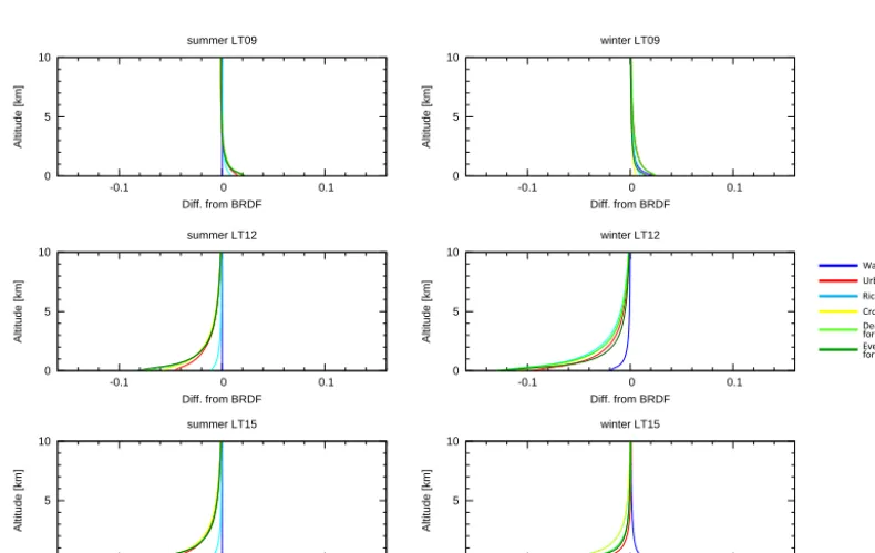
Figure 10 shows the relative differences of the BAMFs for BSA (BBSA) from the BAMF for full BRDF treatment
(BBRDF). The results forBBRF andBWSA are shown in the
Supplement. The differences fromBBRDFbecomes larger in
the lower altitudes, and the differences can be larger than 10 %. The results forBBRFandBWSAare also similar to the
results for BBRDF. This suggests that using BRF, BSA, or
WSA instead of BRDF as an approximation of the surface albedo causes an error which depends on where the NO2is
located in the atmosphere, the difference becoming large if a high concentration of NO2exists in the lowest layers.
Fig-ure 10 suggests that the tropospheric VCD of NO2will be
un-derestimated in the morning (due to larger BAMF) and over-estimated in the afternoon (due to smaller BAMF) in the case of the BSA approximation. In the winter case, for example, the amounts of the underestimation and overestimation reach 15 and 9 %, respectively, when we assume 10 times larger concentration of NO2in the lowest layer (0–1 km altitude).
Note that the occurrence of underestimation or overestima-tion depends on the relative azimuth and thus the locaoverestima-tion of the satellite. In other words, the local time dependence depends on whether the relative location of a geostationary satellite is west or east of the observation point on the sur-face. In the present study, the satellite is assumed to be lo-cated in the west of the observation point. If the location of the satellite is different, the result will be different.
Heckel et al. (2011) also obtained a similar result for the combination of wrong surface albedo and a high concentra-tion of NO2; the authors showed a case where large AMF
errors occurred if the surface albedo was wrong due to the coarse spatial resolution and if a high concentration of NO2
exists only over such a surface. In that case, the AMF value changed from 0.7 to 0.4 if they used MODIS-BSA (higher
resolution) instead of GOME-LER (lower resolution) for sur-face reflectance.
3.4 Effect of aerosols
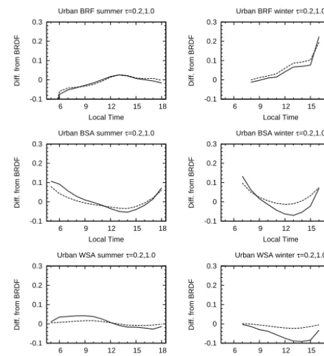
Figure 11 shows the relative difference of the AMFs for ap-proximated BRDF surface types, ABRF,ABSA, andAWSA,
from the AMF for BRDF,ABRDFfor AOD of 1.0. For better
comparison, Figure 10 shows only the results for the urban type at different AOD values (0.2 and 1.0). Again, we as-sume the constant NO2profile shown in Fig. 4. Compared
with Fig. 7, where AOD of 0.2 is assumed, smaller variabil-ity of AMF can be seen among land cover types in Fig. 11. In other words, the values of AMF for all land cover types tend to converge in Fig. 11. This can be attributed to the fact that larger scattering of aerosols weakens the importance of the surface term on the radiation field and thus decreases the dependence on the BRDF of different land cover types. Fig-ure 10 indicates that the AMF computed using the WSA has the smallest difference from that based on the full BRDF. This suggests that not considering the angular dependence at all (i.e., WSA) is better than an incomplete implementation (i.e., BRF and BSA) of angle dependence. In summary, the importance of BRDF on the AMFs decreases for increasing AOD.
3.5 Effect of the AMF differences on the NO2VCDs
Finally, we estimated the effect of the AMF differences men-tioned above on the retrievals of tropospheric NO2 VCDs.
In this estimate, we neglect the effect of stratospheric NO2
and assume that the tropospheric NO2slant column density
(SCD) can be obtained precisely. Assuming that the tropo-spheric NO2 VCD calculated by using BRDF is the true
value, we calculated the relative difference or “error”Ei of
the tropospheric NO2VCD for an albedo typei(i.e., BRF,
BSA, and WSA) from the true VCD as follows:
Ei =(Vi−Vtrue) / Vtrue, (4)
wherei denotes BRF, BSA, and WSA, Vi=SBRDF/ Ai is
the tropospheric NO2 VCD for the albedo type i, Vtrue=
SBRDF/ ABRDFis the true tropospheric NO2VCD, which is
calculated by using BRDF, andV andSare VCD and SCD, respectively.
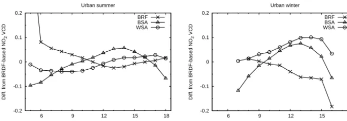
Figure 13 shows theEifor the urban surface type. We can
see that the difference is up to 10 % in most cases, and the occurrence of underestimation or overestimation depends on season and local time. Focusing on BSA, for example, sev-eral percent of underestimation occurs in the early morning, and a similar amount of overestimation occurs in the after-noon. In the Supplement, results for other albedo types are shown. Except for the water type and the summer case of the rice paddy type, the seasonal and local time variations of allEi are similar, which is expected from the results for the
0 5 10
0 1 2 3
Altitude [km]
BAMF summer LT12
0 5 10
0 1 2 3
Altitude [km]
BAMF winter LT12
Fig. 9. TroposphericNO2BAMF at local time (LT) 12 in summer (left) and winter (right) using BRDF surface.
The colors indicate land cover types: water (blue), urban (red), rice paddy (light blue), crop (yellow), deciduous
forest (light green) and evergreen forest (green). An aerosol optical depth (AOD) of 0.2 is assumed.
26
Figure 9. Tropospheric NO2BAMF at 12:00 local time (LT) in summer (left) and winter (right) using BRDF surface. The colors indicate land cover types: water (blue), urban (red), rice paddy (light blue), crop (yellow), deciduous forest (light green), and evergreen forest (green). An aerosol optical depth (AOD) of 0.2 is assumed.
0 5 10
-0.1 0 0.1
Altitude [km]
Diff. from BRDF summer LT09
0 5 10
-0.1 0 0.1
Altitude [km]
Diff. from BRDF summer LT12
0 5 10
-0.1 0 0.1
Altitude [km]
Diff. from BRDF summer LT15
0 5 10
-0.1 0 0.1
Altitude [km]
Diff. from BRDF winter LT09
0 5 10
-0.1 0 0.1
Altitude [km]
Diff. from BRDF winter LT12
0 5 10
-0.1 0 0.1
Altitude [km]
Diff. from BRDF winter LT15
Fig. 10. Relative difference of troposphericNO2BAMF for various land cover types from the tropospheric
NO2BAMF obtained using full BRDF treatment compared to results implementing the values of BSA surface
as LER in the RTM. Panels at local time (LT) 09, LT12 and LT15 for summer (left) and winter (right) are shown.
The colors indicate land cover types: water (blue), urban (red), rice paddy (light blue), crop (yellow), deciduous
forest (light green) and evergreen forest (green). An aerosol optical depth (AOD) of 0.2 is assumed.
27
Figure 10. Relative difference of tropospheric NO2BAMF for various land cover types from the tropospheric NO2BAMF obtained using full BRDF treatment compared to results implementing the values of BSA surface as LER in the RTM. Panels at 09:00, 12:00, and 15:00 LT for summer (left) and winter (right) are shown. The colors indicate land cover types: water (blue), urban (red), rice paddy (light blue), crop (yellow), deciduous forest (light green), and evergreen forest (green). An aerosol optical depth (AOD) of 0.2 is assumed.
3506 K. Noguchi et al.: BRDF effect on GEO measurements 0
0.5 1 1.5
6 9 12 15 18
Trop. AMF Local Time τ 0 0.5 1 1.5
6 9 12 15 18
Trop. AMF Local Time τ -0.1 0 0.1 0.2 0.3
6 9 12 15 18
Diff. from BRDF
Local Time BRF summer τ=1.0
-0.1 0 0.1 0.2 0.3
6 9 12 15 18
Diff. from BRDF
Local Time BRF winter τ=1.0
0 0.5 1 1.5
6 9 12 15 18
Trop. AMF
Local Time BSA summer τ=1.0
0 0.5 1 1.5
6 9 12 15 18
Trop. AMF
Local Time BSA winter τ=1.0
-0.1 0 0.1 0.2 0.3
6 9 12 15 18
Diff. from BRDF
Local Time BSA summer τ=1.0
-0.1 0 0.1 0.2 0.3
6 9 12 15 18
Diff. from BRDF
Local Time BSA winter τ=1.0
0 0.5 1 1.5
6 9 12 15 18
Trop. AMF
Local Time WSA summer τ=1.0
0 0.5 1 1.5
6 9 12 15 18
Trop. AMF
Local Time WSA winter τ=1.0
-0.1 0 0.1 0.2 0.3
6 9 12 15 18
Diff. from BRDF
Local Time WSA summer τ=1.0
-0.1 0 0.1 0.2 0.3
6 9 12 15 18
Diff. from BRDF
Local Time WSA winter τ=1.0
Fig. 11. Relative difference of troposphericNO2AMFs from the value obtained with full BRDF treatment
when implementing the values of BRF (top), BSA (middle) and WSA (bottom) surface as LER in the RTM in
summer (left) and winter (right). The colors indicate land cover types: water (blue), urban (red), rice paddy
(light blue), crop (yellow), deciduous forest (light green) and evergreen forest (green). An aerosol optical depth
(AOD) of 1.0 is assumed.
28
Figure 11. Relative difference of tropospheric NO2AMFs from the value obtained with full BRDF treatment when implementing the values of BRF (top), BSA (middle), and WSA (bottom) surface as LER in the RTM in summer (left) and winter (right). The colors indicate land cover types: water (blue), urban (red), rice paddy (light blue), crop (yellow), deciduous forest (light green), and evergreen forest (green). An aerosol optical depth (AOD) of 1.0 is assumed.
4 Concluding remarks
Assuming a geostationary satellite monitoring, we investi-gated the effect of surface reflectance anisotropy, BRDF, on the tropospheric NO2 measurements by calculating AMF
and BAMF for different BRDF types. Besides BRDF, which fully considers surface reflectance anisotropy, we imple-mented three albedo values from different models (BRF, BSA, WSA), which have a different level of the consider-ation of surface reflectance anisotropy as an approximconsider-ation, as LER in RTM. In our calculations, we also considered six land cover types: water, urban, paddy, crop, deciduous forest, and evergreen forest and their respective seasonal BRDFs.
Using MODIS BRDF results with AVNIR-2 land cover map data, we first developed an empirical model of BRDF parameters (fiso, fvol, fgeo) specific to land cover types
rep-resentative of the Tokyo area. Using the empirical model, we calculated AMFs and BAMFs for tropospheric NO2with
SCIATRAN. Results show that the AMF for tropospheric NO2 largely depends on land cover types; the variability
among the land types is up to several tens of percent. If we neglect the reflectance anisotropy (i.e., use BRF, BSA, or WSA), the difference from AMFBRDFreaches 10 % or more.
The difference depends in a complicated way on season and local time. Incomplete implementation of surface reflectance anisotropy (i.e., BRF and BSA) can lead to even worse re-sults than not considering the anisotropy of reflectance at all
0 0.5 1
6 9 12 15 18
Trop. AMF
Local Time
0 0.5 1
6 9 12 15 18
Trop. AMF Local Time -0.1 0 0.1 0.2 0.3
6 9 12 15 18
Diff. from BRDF
Local Time Urban BRF summer τ=0.2,1.0
-0.1 0 0.1 0.2 0.3
6 9 12 15 18
Diff. from BRDF
Local Time Urban BRF winter τ=0.2,1.0
0 0.5 1 1.5
6 9 12 15 18
Trop. AMF
Local Time Urban BSA summer τ=0.2,1.0
0 0.5 1 1.5
6 9 12 15 18
Trop. AMF
Local Time Urban BSA winter τ=0.2,1.0
-0.1 0 0.1 0.2 0.3
6 9 12 15 18
Diff. from BRDF
Local Time Urban BSA summer τ=0.2,1.0
-0.1 0 0.1 0.2 0.3
6 9 12 15 18
Diff. from BRDF
Local Time Urban BSA winter τ=0.2,1.0
0 0.5 1 1.5
6 9 12 15 18
Trop. AMF
Local Time Urban WSA summer τ=0.2,1.0
0 0.5 1 1.5
6 9 12 15 18
Trop. AMF
Local Time Urban WSA winter τ=0.2,1.0
-0.1 0 0.1 0.2 0.3
6 9 12 15 18
Diff. from BRDF
Local Time Urban WSA summer τ=0.2,1.0
-0.1 0 0.1 0.2 0.3
6 9 12 15 18
Diff. from BRDF
Local Time Urban WSA winter τ=0.2,1.0
Fig. 12. Relative difference of troposphericNO2AMFs from the value obtained with full BRDF treatment
when implementing the values of BRF (top), BSA (middle) and WSA (bottom) surface as LER in the RTM
for Urban type in summer (left) and winter (right). Aerosol optical depths (AODs) of 0.2 (solid curve) and 1.0
(broken curve) are assumed, respectively.
29
Figure 12. Relative difference of tropospheric NO2AMFs from the value obtained with full BRDF treatment when implementing the values of BRF (top), BSA (middle), and WSA (bottom) surface as LER in the RTM for urban type in summer (left) and winter (right). Aerosol optical depths (AODs) of 0.2 (solid curve) and 1.0 (dotted curve) are assumed, respectively.
(i.e., WSA). For lower altitudes, the BAMF difference among land cover types becomes larger. The difference of BAMFs computed using the BRF, BSA, and WSA from those de-rived using full BRDF treatment is also larger in the lower layers. If a high concentration of the tropospheric NO2exists
in the lower altitudes, failure to consider variations or BRDF will cause larger errors of the AMF. For example, if we use the BSA approximation instead of BRDF, the amounts of the underestimation (in the morning) and overestimation (in the afternoon) of the tropospheric VCD of NO2 reach 15 and
9 %, respectively, for the very polluted winter case with a 10 times larger concentration of NO2in the lowest layer (0–
1 km altitude). The size and direction of the error depend on the relative location of the satellite to the observation point on the surface. At larger AOD (1.0), the differences in AMFs for the various surface types become smaller as the impor-tance of BRDF decreases for large AOD.
-0.2 -0.1 0 0.1 0.2
6 9 12 15 18
Diff. from BRDF-based NO
2
VCD
Local Time Urban summer
BRF BSA WSA
-0.2 -0.1 0 0.1 0.2
6 9 12 15 18
Diff. from BRDF-based NO
2
VCD
Local Time Urban winter
BRF BSA WSA
Fig. 13. Relative difference of the troposphericNO2VCDs from the value obtained with full BRDF treatment
when implementing the values of BRF, BSA and WSA surface as LER in the RTM in summer (left) and winter
(right). The results for the urban surface type are shown. The VCD for BRDF is assumed to be a true value.
30
Figure 13. Relative difference of the tropospheric NO2VCDs from the value obtained with full BRDF treatment when implementing the values of BRF, BSA, and WSA surface as LER in the RTM in summer (left) and winter (right). The results for the urban surface type are shown. The VCD for BRDF is assumed to be a true value.
with the validation of NO2 column densities by ground
and/or airborne measurements. More comparison and vali-dation of satellite-based BRDF measurements (e.g., Román et al. (2009) for forests; Susaki et al. (2004, 2007) for rice paddies) and the detailed evaluation of the dependence of BRDF parameters on SZA (Jin et al., 2003) will be needed from independent satellite measurements and ground mea-surements.
For real measurements, we also need to consider the prob-lem of mixed surface types since the field of view of the sensor of the GMAP-Asia project is 10 km or less, which would usually include several surface types simultaneously. The present study focused on simple surface types to eval-uate the range of possible effects. Although an exact treat-ment of a mixed BRDF is not straightforward, a good as-sumption would be that the effect of the mixed BRDF on the AMF is just the average of the individual effects, weighted by the contribution of the different surface types included in the field of view of the sensor. The effect of such mixed surface types on real measurements should be evaluated in future studies.
The findings in the present study are based on the geome-try of the sun, an observed point on the ground surface, and a satellite (an observer), and are specific to the geostationary observation assumed in the present study. Detailed analysis for other satellite retrievals will be needed.
The Supplement related to this article is available online at doi:10.5194/amt-7-3497-2014-supplement.
Acknowledgements. We would like to thank Yasuko Kasai and other members of the APOLLO project and the Japan Society of Atmospheric Chemistry. We would also like to thank Kanako Mu-ramatsu and Noriko Soyama for their useful comments on surface albedo. For the calculation of the SZA and other angles, we utilized the website of the National Astronomical Observatory of Japan (http://www.nao.ac.jp/koyomi/koyomix/koyomix.html).
The MODIS products were available at the NASA website,
http://reverb.echo.nasa.gov. The High Resolution Land-Use
and Land-Cover Map is available at the JAXA website, http://www.eorc.jaxa.jp/ALOS/lulc/lulc_jindex.htm. This work was supported by JSPS KAKENHI grant nos. 24710008 (K. Noguchi) and 22310004 (K. Kita). This work was carried out partly by the joint research program of CEReS, Chiba University (2013). This research was partly supported by the Coordination Funds for Promoting Space Utilization of the Ministry of Education, Culture, Sports, Science and Technology (MEXT), JAPAN.
Edited by: S. Beirle
References
Akimoto, H., Kasai, Y., and Kita, K., (Eds.): Planning a Geosta-tionary Atmospheric Observation Satellite, National Institute of Information and Communications Technology, 2008.
Akimoto, H., Kasai, Y., Kita, K., Irie, H., Sagi, K., and Hayashida, S.: Geostationary Atmospheric Observation Satellite Plan in Japan (Invited), AGU Fall Meeting Abstracts, A51M–01, 2009. Boersma, K. F., Eskes, H. J., Dirksen, R. J., van der A, R. J.,
Veefkind, J. P., Stammes, P., Huijnen, V., Kleipool, Q. L., Sneep, M., Claas, J., Leitão, J., Richter, A., Zhou, Y., and Brunner, D.:
An improved tropospheric NO2column retrieval algorithm for
the Ozone Monitoring Instrument, Atmos. Meas. Tech., 4, 1905– 1928, doi:10.5194/amt-4-1905-2011, 2011.
Bovensmann, H., Burrows, J. P., Buchwitz, M., Frerick, J., Noël, S., Rozanov, V. V., Chance, K. V., and Goede, A. P. H.: SCIAMACHY: Mission Objectives and Measure-ment Modes, J. Atmos. Sci., 56, 127–150, doi:10.1175/1520-0469(1999)056<0127:SMOAMM>2.0.CO;2, 1999.
Burrows, J. P., Weber, M., Buchwitz, M., Rozanov, V., Ladstätter-Weißenmayer, A., Richter, A., Debeek, R., Hoogen, R., Bramstedt, K., Eichmann, K.-U., Eisinger, M., and Perner, D.: The Global Ozone Monitoring Experiment (GOME): Mission Concept and First Scientific Results, J. Atmos. Sci., 56, 151–175, doi:10.1175/1520-0469(1999)056<0151:TGOMEG>2.0.CO;2, 1999.
Callies, J., Corpaccioli, E., Eisinger, M., Hahne, A., and Lefebvre, A.: GOME-2 Metop’s second-generation sensor for operational ozone monitoring, ESA Bulletin, 102, 28–36, 2000.
Fukue, K., Igarashi, T., Osawa, Y., Shimoda, H., Matsuoka, R., and Kawata, Y.: Advanced Visible and Near-Infrared Radiometer type 2 (AVNIR-2), Proc. SPIE, 2957, 208–215, 1997.
Grell, G. A., Peckham, S. E., Schmitz, R., McKeen, S. A., Frost, G., Skamarock, W. C., and Eder, B.: Fully coupled “online” chem-istry within the WRF model, Atmos. Environ., 39, 6957–6975, doi:10.1016/j.atmosenv.2005.04.027, 2005.
Heckel, A., Kim, S.-W., Frost, G. J., Richter, A., Trainer, M., and Burrows, J. P.: Influence of low spatial resolution a priori data
on tropospheric NO2satellite retrievals, Atmos. Meas. Tech., 4,
1805–1820, doi:10.5194/amt-4-1805-2011, 2011.
Hess, M., Koepke, P., and Schult, I.: Optical Properties of Aerosols and Clouds: The Software Package OPAC, Bull. Amer. Meteorol. Soc., 79, 831–844, doi:10.1175/1520-0477(1998)079<0831:OPOAAC>2.0.CO;2, 1998.
Jacob, D. J., Crawford, J. H., Kleb, M. M., Connors, V. S., Bendura, R. J., Raper, J. L., Sachse, G. W., Gille, J. C., Emmons, L., and Heald, C. L.: Transport and Chemical Evolution over the Pacific (TRACE-P) aircraft mission: Design, execution, and first results, J. Geophys. Res., 108, 9000, doi:10.1029/2002JD003276, 2003. Jin, Y., Schaaf, C. B., Woodcock, C. E., Gao, F., Li, X., Strahler, A. H., Lucht, W., and Liang, S.: Consistency of MODIS surface bidirectional reflectance distribution function and albedo retrievals: 2. Validation, J. Geophys. Res., 108, 4159, doi:10.1029/2002JD002804, 2003.
Justice, C., Vermote, E., Townshend, J., Defries, R., Roy, D., Hall, D., Salomonson, V., Privette, J., Riggs, G., Strahler, A., Lucht, W., Myneni, R., Knyazikhin, Y., Running, S., Nemani, R., Wan, Z., Huete, A., van Leeuwen, W., Wolfe, R., Giglio, L., Muller, J., Lewis, P., and Barnsley, M.: The Moderate Resolution Imag-ing Spectroradiometer (MODIS): land remote sensImag-ing for global change research, IEEE Trans. Geosci. Remote Sens., 36, 1228– 1249, doi:10.1109/36.701075, 1998.
Levelt, P. F., van den Oord, G. H. J., Dobber, M. R., Malkki, A., Visser, H., de Vries, J., Stammes, P., Lundell, J. O. V., and Saari, H.: The ozone monitoring instrument, IEEE Trans. Geosci. Remote Sens., 44, 1093–1101, doi:10.1109/TGRS.2006.872333, 2006.
Lin, J.-T., Martin, R. V., Boersma, K. F., Sneep, M., Stammes, P., Spurr, R., Wang, P., Van Roozendael, M., Clémer, K., and Irie, H.: Retrieving tropospheric nitrogen dioxide over China from the Ozone Monitoring Instrument: effects of aerosols, surface reflectance anisotropy and vertical profile of nitro-gen dioxide, Atmos. Chem. Phys. Discuss., 13, 21203–21257, doi:10.5194/acpd-13-21203-2013, 2013.
Lucht, W., Schaaf, C., and Strahler, A.: An algorithm for the retrieval of albedo from space using semiempirical BRDF models, IEEE Trans. Geosci. Remote Sens., 38, 977–998, doi:10.1109/36.841980, 2000.
Nicodemus, F. E., Richmond, J. C., Hsia, J. J., Ginsberg, I. W., and Limperis, T.: Geometrical considerations and nomenclature for reflectance, NBS MN-160, Natl. Bur. Stand. Rep., 1977. Noguchi, K., Richter, A., Bovensmann, H., Hilboll, A., Burrows,
J. P., Irie, H., Hayashida, S., and Morino, Y.: A feasibility study
for the detection of the diurnal variation of tropospheric NO2
over Tokyo from a geostationary orbit, Adv. Space Res., 48, 1551–1564, doi:10.1016/j.asr.2011.06.029, 2011.
Noguchi, K., Richter, A., Burrows, J. P., Irie, H., and Kita, K.: A study of BRDF over Tokyo for the spaceborne
measure-ments of atmospheric trace gases, Proc. SPIE, 8524 pp., 85242D, doi:10.1117/12.974818, 2012.
Román, M. O., Schaaf, C. B., Woodcock, C. E., Strahler, A. H., Yang, X., Braswell, R. H., Curtis, P. S., Davis, K. J., Dragoni, D., Goulden, M. L., Gu, L., Hollinger, D. Y., Kolb, T. E., Mey-ers, T. P., Munger, J. W., Privette, J. L., Richardson, A. D., Wil-son, T. B., and Wofsy, S. C.: The MODIS (Collection V005) BRDF/albedo product: Assessment of spatial representativeness over forested landscapes, Remote Sens. Environ., 113, 2476– 2498, doi:10.1016/j.rse.2009.07.009, 2009.
Roujean, J.-L., Leroy, M., and Deschanps, P.-Y.: A bidirectional reflectance model of the Earth’s surface for the correction of remote sensing data, J. Geophys. Res., 97, 20455–20468, doi:10.1029/92JD01411, 1992.
Rozanov, A., Rozanov, V., Buchwitz, M., Kokhanovsky, A., and Burrows, J. P.: SCIATRAN 2.0–A new radiative transfer model for geophysical applications in the 175–2400 nm spectral region, Adv. Space Res., 36, 1015–1019, doi:10.1016/j.asr.2005.03.012, 2005.
Rozanov, V., Rozanov, A., Kokhanovsky, A., and Burrows, J.: Ra-diative transfer through terrestrial atmosphere and ocean: Soft-ware package SCIATRAN, J. Quant. Spectr. Rad. Trans., 133, 13–71, doi:10.1016/j.jqsrt.2013.07.004, 2014.
Russell, A. R., Perring, A. E., Valin, L. C., Bucsela, E. J., Browne, E. C., Wooldridge, P. J., and Cohen, R. C.: A high
spa-tial resolution retrieval of NO2 column densities from OMI:
method and evaluation, Atmos. Chem. Phys., 11, 8543–8554, doi:10.5194/acp-11-8543-2011, 2011.
Schaaf, C. B., Gao, F., Strahler, A. H., Lucht, W., Li, X., Tsang, T., Strugnell, N. C., Zhang, X., Jin, Y., Muller, J.-P., Lewis, P., Barnsley, M., Hobson, P., Disney, M., Roberts, G., Dunderdale, M., Doll, C., d’Entremont, R. P., Hu, B., Liang, S., Privette, J. L., and Roy, D.: First operational BRDF, albedo nadir reflectance products from MODIS, Remote Sens. Environ., 83, 135–148, doi:10.1016/S0034-4257(02)00091-3, 2002.
Sudo, K., Takahashi, M., Kurokawa, J., and Akimoto,
H.: CHASER: A global chemical model of the tropo-sphere 1. Model description, J. Geophys. Res., 107, 4339, doi:10.1029/2001JD001113, 2002.
Susaki, J., Hara, K., Park, J., Yasuda, Y., Kajiwara, K., and Honda, Y.: Validation of temporal BRDFs of paddy fields estimated from MODIS reflectance data, IEEE Trans. Geosci. Remote Sens., 42, 1262–1270, doi:10.1109/TGRS.2004.826798, 2004.
Susaki, J., Yasuoka, Y., Kajiwara, K., Honda, Y., and Hara, K.: Validation of MODIS Albedo Products of Paddy Fields in Japan, IEEE Trans. Geosci. Remote Sens., 45, 206–217, doi:10.1109/TGRS.2006.882266, 2007.
Takigawa, M., Niwano, M., Akimoto, H., and Takahashi, M.: Devel-opment of a one-way nested global-regional air quality forecast-ing model, SOLA, 3, 81–84, doi:10.2151/sola.2007-021, 2007. Zhou, Y., Brunner, D., Boersma, K. F., Dirksen, R., and Wang, P.:
An improved tropospheric NO2retrieval for OMI observations
in the vicinity of mountainous terrain, Atmos. Meas. Tech., 2, 401–416, doi:10.5194/amt-2-401-2009, 2009.
Zhou, Y., Brunner, D., Spurr, R. J. D., Boersma, K. F., Sneep, M., Popp, C., and Buchmann, B.: Accounting for surface reflectance
anisotropy in satellite retrievals of tropospheric NO2, Atmos.