University of Pennsylvania
ScholarlyCommons
Publicly Accessible Penn Dissertations
2018
Formally Verified Quantum Programming
Robert Rand
University of Pennsylvania, [email protected]
Follow this and additional works at:https://repository.upenn.edu/edissertations Part of theComputer Sciences Commons
This paper is posted at ScholarlyCommons.https://repository.upenn.edu/edissertations/3175 Recommended Citation
Rand, Robert, "Formally Verified Quantum Programming" (2018).Publicly Accessible Penn Dissertations. 3175.
Formally Verified Quantum Programming
Abstract
The field of quantum mechanics predates computer science by at least ten years, the time between the
publication of the Schrodinger equation and the Church-Turing thesis. It took another fifty years for Feynman to recognize that harnessing quantum mechanics is necessary to efficiently simulate physics and for David Deutsch to propose the quantum Turing machine. After thirty more years, we are finally getting close to the first general-purpose quantum computers based upon prototypes by IBM, Intel, Google and others.
While physicists and engineers have worked on building scalable quantum computers, theoretical computer scientists have made their own advances. Complexity theorists introduced quantum complexity classes like BQP and QMA; Shor and Grover developed their famous algorithms for factoring and unstructured search. Programming languages researchers pursued two main research directions: Small-scale languages like QPL and the quantum lambda-calculi for reasoning about quantum computation and large-scale languages like Quipper and Q# for industrial-scale quantum software development. This thesis aims to unify these two threads while adding a third one: formal verification.
We argue that quantum programs demand machine-checkable proofs of correctness. We justify this on the basis of the complexity of programs manipulating quantum states, the expense of running quantum programs, and the inapplicability of traditional debugging techniques to programs whose states cannot be examined. We further argue that the existing mathematical models of quantum computation make this an easier task than one could reasonably expect. In light of these observations we introduce QWIRE, a tool for writing verifiable, large scale quantum programs.
QWIRE is not merely a language for writing and verifying quantum circuits: it is a verified circuit description language. This means that the semantics of QWIRE circuits are verified in the Coq proof assistant. We also implement verified abstractions, like ancilla management and reversible circuit compilation. Finally, we turn QWIRE and Coq's abilities outwards, towards verifying popular quantum algorithms like quantum
teleportation. We argue that this tool provides a solid foundation for research into quantum programming languages and formal verification going forward.
Degree Type Dissertation
Degree Name
Doctor of Philosophy (PhD)
Graduate Group
Computer and Information Science
First Advisor Steve Zdancewic
Keywords
FORMALLY VERIFIED QUANTUM
PROGRAMMING
Robert Rand
A DISSERTATION
in
Computer and Information Science
Presented to the Faculties of the University of Pennsylvania
in
Partial Fulfillment of the Requirements for the
Degree of Doctor of Philosophy
2018
Supervisor of Dissertation
Steve Zdancewic
Professor of Computer and Information Science
Graduate Group Chairperson
Rajeev Alur
Professor of Computer and Information Science
Dissertation Committee
Stephanie Weirich, Professor of Computer and Information Science, Chair
Val Tannen, Professor of Computer and Information Science
Benjamin Pierce, Professor of Computer and Information Science
Acknowledgments
A lot of people helped me on the road to this dissertation, none more than my advisor, Steve Zdancewic. From the moment I wandered into his office and asked if we could do research on probability and logic (his response: “Sure!”), to the moment he emailed me and Jennifer Paykin asking if we wanted to work on a quantum computing project (“Sure!”), to the moment I submitted this dissertation, Steve has been endlessly enthusiastic, generous with his time, and willing to explore entirely new horizons.
In a similar vein, I have to thank my friend and collaborator Jennifer Paykin, who jumped into the new and exciting world of quantum programming languages with me. Doing research is an entirely different, and better, experience with a close collaborator, especially one as talented and tireless as Jennifer.Qwire, and therefore this thesis, could not possibly have existed without her.
Thanks to Mike Mislove and the other members of the “Semantics, Formal Rea-soning, and Tools for Quantum Programming” research initiative for introducing me to quantum computing and helping me acclimate to the field. Relatedly, thanks to the MFPS and QPL communities, which taught me a great deal and always made me feel welcome. Thanks especially to Peter Selinger, who blazed the path that I tried to follow and happily helped me along it, and Prakash Panangaden, who lent me his knowledge of quantum mechanics and graciously agreed to serve on my thesis committee.
Thanks to Andy Gordon, who hosted me for a summer at Microsoft Research Cambridge. Thanks to my collaborators there: Neil Toronto, Cecily Morrison, Claudio Russo, Simon Peyton-Jones, Abigail Sellen, Felienne Hermans, Advait Sarkar and Rupert Horlick. Also, thanks to Tony Hoare, Cédric Fournet and Georges Gonthier for intellectually stimulating lunch meetings that often segued into extensive discussions of formal verification.
Jesús Gallego Arias and Benoît Valiron for their generous help and camaraderie. Everyone who read this thesis, in part or in full, has my lasting gratitude. That’s Steve and Jennifer again, and my committee, Stephanie, Benjamin, Val and Prakash, as well Julien Ross, Yannick Zakowski, Alex Burka and Rivka Cohen. You are all my heroes.
ABSTRACT
FORMALLY VERIFIED QUANTUM PROGRAMMING
Robert Rand
Steve Zdancewic
The field of quantum mechanics predates computer science by at least ten years, the time between the publication of the Schrödinger equation and the Church-Turing thesis. It took another fifty years for Feynman to recognize that harnessing quantum mechanics is necessary to efficiently simulate physics and for David Deutsch to propose the quantum Turing machine. After thirty more years, we are finally getting close to the first general-purpose quantum computers based upon prototypes by IBM, Intel, Google and others.
While physicists and engineers have worked on building scalable quantum comput-ers, theoretical computer scientists have made their own advances. Complexity theo-rists introduced quantum complexity classes like BQP and QMA; Shor and Grover de-veloped their famous algorithms for factoring and unstructured search. Programming languages researchers pursued two main research directions: Small-scale languages like QPL and the quantum λ-calculi for reasoning about quantum computation and large-scale languages like Quipper and Q# for industrial-scale quantum software de-velopment. This thesis aims to unify these two threads while adding a third one:
formal verification.
We argue that quantum programs demand machine-checkable proofs of correct-ness. We justify this on the basis of the complexity of programs manipulating quan-tum states, the expense of running quanquan-tum programs, and the inapplicability of traditional debugging techniques to programs whose states cannot be examined. We further argue that the existing mathematical models of quantum computation make this an easier task than one could reasonably expect. In light of these observations we introduce Qwire, a tool for writing verifiable, large scale quantum programs.
Qwireis not merely a language for writing and verifying quantum circuits: it is a
Contents
List of Figures ix
List of Tables x
1 The Big Picture 1
1.1 Motivation . . . 1
1.2 Thesis Statement . . . 4
1.3 Outline . . . 4
2 An Introduction to Quantum Computing 7 2.1 Qubits . . . 7
2.2 Example: Quantum Teleportation . . . 11
2.3 Quantum Circuits . . . 12
2.4 Quantum States as Vectors . . . 13
2.4.1 Unitary transformations . . . 14
2.5 Mixed States as Density Matrices . . . 17
2.6 Additional Material . . . 20
3 History 21 3.1 Circuits, QRAM and Classical Control . . . 21
3.2 QCL: A General Purpose Quantum Language . . . 22
3.3 QPL: Semantics for Quantum Programming . . . 23
3.4 Linearity and the Quantum Lambda Calculi . . . 25
3.5 The Quantum IO Monad . . . 27
3.6 Quipper and the Proto-Quippers . . . 27
3.7 Liquid, Revs and Q# . . . 29
3.8 The World of Quantum Programming . . . 30
3.9 Models of Quantum Computation . . . 30
3.10 Formal Verification . . . 31
3.10.1 Quantum Logics . . . 32
4 Qwire in Theory 34
4.1 Introduction . . . 34
4.1.1 The Best of Both Worlds: Qwire . . . 35
4.1.2 Chapter Outline . . . 36
4.2 Qwire by Example . . . 37
4.3 The Qwire Circuit Language . . . 40
4.3.1 Circuit Language . . . 40
4.3.2 Host Language . . . 41
4.3.3 Static Semantics . . . 43
4.4 Operational Semantics: Circuit Normalization . . . 45
4.4.1 Type Safety . . . 49
4.5 Denotational Semantics . . . 50
4.5.1 Operational Behavior of run . . . 53
4.6 A Categorical Semantics for Qwire . . . 53
4.7 Dependent Types . . . 54
4.8 Summary . . . 55
5 Qwire in Practice 57 5.1 Circuits in Coq . . . 57
5.2 Typing Qwire . . . 59
5.3 De Bruijin Circuits . . . 61
5.4 Matrices and Semantics . . . 63
5.4.1 Complex Numbers . . . 63
5.4.2 The Matrix Library . . . 64
5.4.3 Density Matrices . . . 65
5.5 Denotation of Qwire . . . 65
5.6 Functional Notations . . . 69
6 Verifying Qwire 73 6.1 Predicates and Preservation . . . 73
6.1.1 Well-Formed Matrices . . . 73
6.1.2 Unitarity . . . 74
6.1.3 Pure and Mixed States . . . 75
6.1.4 Superoperator Correctness . . . 76
6.2 Towards Compositionality . . . 77
6.3 Future Work on Qwire’s Metatheory . . . 78
7 Verifying Quantum Programs 80 7.1 Verifying Matrices . . . 80
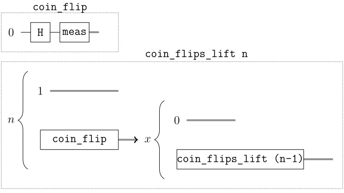
7.1.1 Tossing Coins . . . 80
7.1.2 Teleport . . . 80
7.1.3 Deutsch’s Algorithm . . . 82
7.2.1 Many Coins . . . 83
7.3 Algebraic Reasoning about Circuits . . . 84
7.3.1 A Unitary and Its Adjoint . . . 84
7.4 Equational Rewriting . . . 85
8 Reversibility 87 8.1 Ancillae and Assertions . . . 87
8.2 Safe and Unsafe Semantics . . . 90
8.3 Syntactically Valid Ancillae . . . 92
8.4 Compiling Oracles . . . 94
8.5 Quantum Arithmetic in Qwire . . . 97
8.6 Next Steps for Reversible Computation . . . 98
9 Automation 100 9.1 Typechecking Circuits . . . 100
9.1.1 Monoid . . . 104
9.1.2 Validate . . . 105
9.2 Arithmetic . . . 105
9.3 Linear Algebra . . . 106
9.3.1 Matrix Properties . . . 106
9.3.2 Solving Matrix Equalities . . . 108
9.4 Denoting Circuits . . . 109
9.5 Tactics Reference . . . 110
10 Details: Qwire Within 113 10.1 An outline ofQwire . . . 113
10.2 Matters of Trust . . . 116
11 Open Wires and Loose Ends 119 11.1 Computing inQwire . . . 119
11.2 Connecting Qwire . . . 121
11.3 The Future of Qwire . . . 121
11.3.1 Verified Optimization and Compilation . . . 122
11.3.2 Error Awareness and Error Correction . . . 123
11.3.3 Verified Algorithms and Cryptography . . . 123
A Solutions to Exercises 125 B Qwire in Theory: Proofs 130 B.1 Type safety and normalization . . . 130
C Qwire Documentation 137
C.1 Prelim.v . . . 137
C.2 Monad.v . . . 137
C.3 Monoid.v . . . 137
C.4 Matrix.v . . . 137
C.5 Quantum.v . . . 137
C.6 Contexts.v . . . 137
C.7 HOASCircuits.v . . . 138
C.8 DBCircuits.v . . . 138
C.9 Denotation.v . . . 138
C.10 HOASLib.v . . . 138
C.11 SemanticLib.v . . . 138
C.12 HOASExamples.v . . . 138
C.13 HOASProofs.v . . . 138
C.14 Equations.v . . . 138
C.15 Composition.v . . . 138
C.16 Ancilla.v . . . 139
C.17 Symmetric.v . . . 139
C.18 Oracles.v . . . 139
List of Figures
2.1 A quantum teleportation circuit . . . 13
3.1 A QPL program for tossing a quantum coin . . . 24
3.2 A quantum teleportation circuit . . . 26
4.1 A Qwire implementation of quantum teleportation without dynamic lifting. . . 38
4.2 Typing rules forQwire. . . 44
4.3 Operational semantics of concrete circuits. . . 48
4.4 Denotational semantics of circuits. . . 52
5.1 Rearranged Typing Rules . . . 60
5.2 A zipper for denoting controlled unitaries . . . 68
5.3 The Deutch-Jozsa circuit . . . 71
5.4 Flipping coins with dynamic lifting . . . 72
7.1 The superdense coding protocol with boolean inputs . . . 81
7.2 Tossing n coins . . . 83
8.1 Quantum oracles implementing the boolean ∧ and ∨. The ⊕ gates represent negation, and ● represents control. . . 87
8.2 An non-unitary quantum oracle for (a∨b)∧(c∨d) . . . 88
8.3 A unitary quantum oracle for (a∨b)∧(c∨d) with ancillae . . . 88
8.4 Compiling b1∧b2 on 3 qubits . . . 96
8.5 A quantum adder . . . 97
9.1 Typing a simple Qwire program . . . 100
9.2 Manually typechecking cnot12. . . 101
List of Tables
8.1 Reversibility assumptions . . . 90
9.1 A summary of Qwire tactics . . . 112
9.2 A summary of Qwire databases . . . 112
10.1 A brief summary of the Qwire Coq development . . . 114
10.2 The claims of Qwire . . . 117
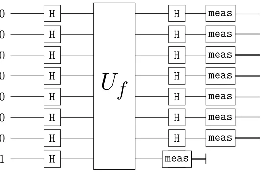
Chapter 1
The Big Picture
1.1
Motivation
In 1936, Alonzo Church wrote a programming language for a machine that didn’t exist. His lambda calculus (Church, 1936a) influenced many of the programming lan-guages that would emerge with the advent of the programmable computer in the 1940s. This, of course, wasn’t Church’s goal: He had in his sights Hilbert’s Entschei-dungsproblem, which asked whether one could write an algorithm to prove arbitrary statements in first-order logic. Church (1936b) and Turing (1937) both answered this problem in the negative and, in doing so, proposed “universal” models of computation that fundamentally ignored the scientific revolution of ten years prior.
While Church and Turing’s models of computation were able to express which problems were computable in theory, they were woefully ill-equipped to describe which problems were solvable in practice, even using the language of complexity theory. Richard Feynman first recognized this in 1982 (Feynman, 1982), pointing out that a Turing machine was seemingly incapable of efficiently simulating physics, since physics obeys the mathematically complex laws of quantum mechanics. This shortcoming was both surprising and disappointing: You would expect that we could simulate basic physical processes on our so-called universal computers.
such as Raz and Avishay’s (2018) proof of an oracle separation between BQP and the polynomial hierarchy. By now, Quantum Complexity Theory is featured in standard complexity theory textbooks (for example, Arora and Barak (2009)) and even books aimed at a popular audience (Aaronson, 2013).
While the complexity theorists and algorithms designers have done an impres-sive job of telling future quantum programmers what to program, programming lan-guages researchers have lagged behind in telling them howto program. This presents a dilemma. When general-purpose quantum computers see the light of day (soon, judging by recent efforts at technology giants Google1, IBM2, Intel3, Microsoft4 and Alibaba5, as well as the start-up Rigetti Computing6), people will program them. And if they are forced to invent ad-hoc programming languages to address the chal-lenges of the moment, we risk introducing design flaws that will plague generations of quantum programmers.
Reassuringly, programming languages research has a head start on actual tum computers. Several important paradigms have gained traction within the quan-tum programming languages community, including the QRAM model (Knill, 1996), in which a quantum computer is used as a sort of oracle by a connected classical computer, and Selinger’s (2004a) refinement called quantum data, classical control, in which data may be quantum, but a program’s control flow is always classical. A special case of Selinger’s approach is the quantum circuit model, in which a classical computer constructs quantum circuits and sends them to a quantum computer for execution.
The twenty-two years since Knill wrote his “Conventions for Quantum Pseu-docode” (Knill, 1996) have seen the proliferation of quantum programming languages, which we can loosely classify into two groups:
1. Academic programming languages for reasoning about quantum programs
2. High level languages for implementing complex quantum programs on future quantum devices
In the first category we have languages like QPL (Selinger, 2004a), λq (van Ton-der, 2004), and the Quantum Lambda Calculus (Selinger and Valiron, 2009). QPL
1
https://www.technologyreview.com/s/604242/googles-new-chip-is-a-stepping-stone-to-quantum-computing-supremacy
2
https://www.technologyreview.com/s/607887/ibm-nudges-ahead-in-the-race-for-quantum-supremacy
3
https://www.technologyreview.com/s/603165/intel-bets-it-can-turn-everyday-silicon-into-quantum-computings-wonder-material
4
http://www.nature.com/news/inside-microsoft-s-quest-for-a-topological-quantum-computer-1.20774
5
https://medium.com/syncedreview/alibaba-launches-11-qubit-quantum-computing-cloud-service-ad7f8e02cc8
6
was one of the first proposed quantum programming languages, with a denotational semantics given in terms of string diagrams and density matrices. This language was used as a model language in a number of subsequent works, such as Kakutani’s (2009) Hoare-like logic QHL and D’Hondt and Panangaden’s (2006) Quantum Weakest Pre-conditions. Van Tonder’s λq and Selinger and Valiron’s Quantum Lambda Calculus are both adaptations of Church’s lambda calculus to a quantum setting. λq focuses on expressivity and sketches a proof of equivalence to Yao’s (1993) quantum circuit model and thereby to the quantum Turing machine. Selinger and Valiron’s calcu-lus, by contrast, focuses on the language’s linear type system, which enforces the
no-cloning theorem of quantum mechanics by guaranteeing that each qubit is used exactly once. None of these languages are designed for practical quantum computing, however.
By contrast, quantum circuit languages like QCL (Ömer, 2000, 2003), Quip-per (Green et al., 2013a,b), Liquid (Wecker and Svore, 2014), and Q# (Svore et al., 2018) are designed for efficient, general-purpose quantum computing. QCL is a C-like language with support for both classical and quantum computing, where Quipper and Liquid are embedded in Haskell and F#, respectively, and are capable of us-ing these languages’ features and libraries to construct complex families of quantum circuits. Q# (Svore et al., 2018) is a recent standalone successor to Liquid, meant to reduce reliance on F# and provide a programming environment targeted exclu-sively at quantum computing. All of these languages provide optimized compilation to low-level circuits and can simulate quantum computation. Unfortunately, they lack important features of QPL and the Quantum Lambda Calculus, such as denotational semantics and type systems that guarantee circuits are well-formed.
Given the cost and expressive power of quantum computing, we need a program-ming language that fits in both of these categories. It should take advantage of existing programming languages research, which strongly suggests using the quantum circuit model adopted by Quipper and Liquid, as well as their abstractions and optimizations. It must ensure that any quantum program sent to the quantum computer represents a valid quantum mechanical operation, as guaranteed by the Quantum Lambda Cal-culus’ linear type system. And finally, it must be provably safe and easy to reason about, in the style of QPL.
program specification into the most convenient as well.
1.2
Thesis Statement
Quantum programming is not only amenable to formal verification: it demands it.
The overarching goal of this thesis is to write and verify quantum programs to-gether. Towards that end, we introduce a quantum programming language called
Qwire and embed it inside the Coq proof assistant. We give it a linear type system to ensure that it obeys the laws of quantum mechanics and a denotational seman-tics to prove that programs behave as desired. We also formalize the metatheory of
Qwireto ensure that the language itself is well-behaved and only supports physically realizable computation. We use Qwire’s rich type theory and semantic guarantees to implement features that could not be safely implemented in other languages, from circuit families to assertive terminations. And, naturally, we use Qwire to verify existing algorithms from the quantum computing literature.
1.3
Outline
We begin by introducing the basics of quantum computing (Chapter 2). We then take a look at the history of quantum programming languages, from van Tonder’s (2003) quantum lambda calculus to powerful modern languages like Quipper (Green et al., 2013a) and Q# (Svore et al., 2018). That brings us to the core of the thesis, the quantum circuit language Qwire.
Qwire is an embedded circuit generation language for quantum computing. In Chapter 4, we give Qwire a denotational semantics in terms of density matrices, a linear type system that guarantees circuits are well formed, and a dynamic lifting
operation for communication between a classical and a quantum computer.
We embed Qwire inside the Coq proof assistant (Chapter 5), tying its variables to those of Coq’s programming language Gallina, and implementing a typechecking algorithm as a Coq tactic. We also provide a direct translation toQwire’s semantics in terms of density matrices, allowing us to prove properties of generated circuits. These density matrices rely on our own libraries for linear algebra and quantum information theory, together with Coquelicot’s (Boldo et al., 2015) complex num-ber library. We explore Qwire’s metatheory in Chapter 6, showing that well-typed circuits correspond to quantum-mechanically sound functions on quantum states. In chapter Chapter 7, we use the resulting semantics to prove the properties of a number of quantum programs, including quantum teleportation, Deutsch’s algorithm (1985), and a variety of coin flipping protocols.
pro-gramming and formal verification. For the reader who would like to understand the Coq programming language better, we recommend our online tutorial (Rand and de Amorim, 2016) or the more comprehensive “Software Foundations,” which also delves deeply into programming languages and type theory, both of which will aid the reader in digesting this work.
WithQwire in hand, we can begin to explore a type-safe approach to high-level quantum programming (Chapter 8, based on Rand et al. (2018a)). We begin by imple-menting some of the core features of Greenet al.’s Quipper language using dependent types. Quipper makes heavy use of ancillas, temporary qubits that are initialized in some state and discarded in the same state, at least according to the assertions that accompany the discard operation. Unfortunately, Quipper has no way of ensuring that these assertions are true. Worse, the compiler relies upon these assertions, so when an assertion is false, the compiled program is likely to misbehave. We include assertions in the Coq implementation of Qwire and require the programmer to prove them correct before the program will compile. We also provide an assertion-using compiler from boolean expressions toQwirecircuits, and we prove that the generated circuits compute the same functions as the provided expressions.
All of this work requires a significant amount of reasoning, from proving that cir-cuits are well typed to showing that they compute the desired function. As we built
Qwire, we noticed which tasks demanded a lot of our own time and attempted to automate them, for our benefit and that of future users. Chapter 9 discusses the vari-ous forms of automation present inQwire, from the monoidal solver and disjointness checker used by our linear typechecker to the range of tactics used in proving matrix equalities.
Given that most of this dissertation discusses the ideas that underlie Qwire, in Chapter 10 we pause the high-level exposition and delve into the Coq development itself. There we discuss the assumptions that we use inQwireand attempt to justify them. We also include every proof and assumption in this thesis in Appendix C, which we urge the reader to consult, especially if an English-language description proves ambiguous. We also encourage the reader to step through the Coq development itself, available at https://github.com/inQWIRE/QWIRE.
Some of this work appears in two prior papers by Paykin, Rand, and Zdancewic: Paykin et al. (2017) and Rand et al. (2017). The first paper, which introduces the
Qwire language and its type system and denotational semantics, forms the basis for Chapter 4. The second paper contains early details of Qwire’s implementation, along with proofs of some basic circuit equalities. Many of the more interestingQwire proofs, particularly those about its metatheory, have yet to be published.
Chapter 2
An Introduction to Quantum
Computing
In this chapter, we introduce the basics of quantum computation, starting with sim-ple qubits and proceeding to concepts like superposition, entanglement, and unitary transformations. We only assume knowledge of basic linear algebra and try to elide any concepts not directly relevant to this dissertation, particularly those related to the physics of quantum computation. To assist the unfamiliar reader, we have included a number of exercises, which should help them internalize ideas as we present them. Solutions to these exercises are provided in Appendix A.
2.1
Qubits
Qubits, a pun on the ancient unit of measure, “cubit,” are the quantum analogue of bits. While qubits can take on a variety of configurations, called states, the two simplest correspond to the binary 0 and 1 and are written ∣0⟩ and ∣1⟩. We call these the basis states. They may represent different amounts of charge on a wire, or base particles rotating clockwise versus counterclockwise—as in classical computing, the physical implementation of qubits does not concern us.
Conveniently, when describing operations on qubits, we can describe their behavior on basis states and then lift this behavior to more complicated quantum states. One common “classical” operation on qubits is Wolfgang Pauli’s X (or NOT) operator, which behaves like classical negation:
X∣0⟩=∣1⟩ X∣1⟩=∣0⟩
define the controlled-not (or CNOT) operator on two qubit states:
CNOT∣00⟩=∣00⟩ CNOT∣01⟩=∣01⟩
CNOT∣10⟩=∣11⟩ CNOT∣11⟩=∣10⟩
When the first qubit is∣1⟩, the second qubit is negated; otherwise, both qubits are unchanged. The meaning of “controlled-not” should therefore be apparent: The first qubit controls whether the second is negated or not. This notion of control can be generalized as follows: For any operatorf onk qubits, a “controlled”f is an operator onk+1qubits that applies f if the first qubit is ∣1⟩and otherwise applies the identity function. Note that if we iterate the “control” operation, the function will be applied only if all of the controlling qubits (or “controls”) are∣1⟩. The controls themselves are never altered by this operation.
Superposition We now introduce our first “quantum” operation, the Hadamard
H, on one-qubit quantum states:
H∣0⟩=√1 2∣0⟩+
1
√
2∣1⟩
H∣1⟩=√1
2∣0⟩+ − 1
√
2∣1⟩
The scaling factors to the left of∣0⟩and∣1⟩are complex numbers calledamplitudes, and the expression α∣0⟩+β∣1⟩represents a superposition, a weighted combination of
∣0⟩and∣1⟩. This has no analogue in classical physics, but for our purposes “a weighted combination” will suffice. The+symbol here behaves like addition: It is commutative and associative and obeys distributive laws, with both scaling and tensor being a form of multiplication. Additionally, ∣ψ⟩ and −∣ψ⟩ cancel each other out, as we will see in the following example.
H(√1 2∣0⟩+
1
√
2∣1⟩)= 1
√
2H∣0⟩+ 1
√
2H∣1⟩
=√1
2( 1
√
2∣0⟩+ 1
√
2∣1⟩)+ 1
√
2( 1
√
2∣0⟩− 1
√
2∣1⟩)
=1 2∣0⟩+
1 2∣1⟩+
1 2∣0⟩−
1 2∣1⟩ =1
2∣0⟩+ 1 2∣0⟩ =∣0⟩
We see that the Hadamard operator can take a non-basis state to a basis state (this will be true of all our operators).
Exercise 1. Show thatH is its own inverse.
Entanglement Things become more interesting once we combine H and CNOT
operators.
Consider a CNOT applied to two qubits: √1 2∣0⟩+
1 √
2∣1⟩ and ∣0⟩:
CNOT[(√1 2∣0⟩+
1
√
2∣1⟩)⊗∣0⟩]=CNOT( 1
√
2∣00⟩+ 1
√
2∣10⟩)
=√1
2(CNOT∣00⟩)+ 1
√
2(CNOT∣10⟩)
=√1
2∣00⟩+ 1
√
2∣11⟩
In this new state, the two qubits are intertwined with one another: It is no longer possible to express this state as the tensor product of two distinct one-qubit states. We call this state of affairs entanglement, and it is closely related to the dependence
of two random variables in probability theory.
Measurement To see where probability enters the picture, we have to introduce the
measurement operator, meas, which, unlikeX,H and CNOT, can only be expressed as a function on the whole qubit, not its components:
meas(α∣0⟩+β∣1⟩)=⎧⎪⎪⎨⎪⎪
⎩
∣0⟩ with probability ∣α∣2
∣1⟩ with probability ∣β∣2
The modulus of a complex number ∣a+bi∣is √a2+b2, so whenever the imaginary
Note that in any single qubit state α∣0⟩+β∣1⟩, we have ∣α∣2+∣β∣2=1, allowing us to translate amplitudes into probabilities.
We can see that measuring ∣0⟩ always yields ∣0⟩ and similarly for ∣1⟩, since the basis state∣0⟩is really1∣0⟩+0∣1⟩. MeasuringH∣0⟩orH∣1⟩will yield each basis state with one-half probability, since √1
2 2
=(−√1 2)
2 = 1
2. Measurement is idempotent: Once
we have measured a qubit, it enters the basis state∣0⟩or∣1⟩, so measuring it a second time has no impact.
We can easily extend this notion of measurement to a multi-qubit system. If we have the state∑iαi∣i⟩, where∣i⟩ranges over the basis states∣0. . .0⟩through∣1. . .1⟩, the probability that measurement returns ∣i⟩ is ∣αi∣
2
.
What if we want to measure one qubit in a multiple qubit system? Let ∑iαi∣i⟩ represent the part of the state in which the qubit to be measured is ∣0⟩and ∑jβj∣j⟩ represent the part in which the qubit is ∣1⟩. Then the probabilityp0 of measuring our
qubit as ∣0⟩is ∑i∣αi∣2, yielding the state
1
√p
0∑i αi∣i⟩
and similarly for p1 and ∣1⟩. The scaling factor √1pi renormalizes the quantum state
so that the squares of the amplitudes still add up to 1.
For example, suppose we want to measure the first qubit in the state
1 3∣00⟩+
2+i 3 ∣01⟩+
1
√
3∣11⟩.
We can break this up into 1 3∣00⟩+
2+i
3 ∣01⟩ and 1 √
3∣11⟩. The probability of measuring
the qubit as ∣0⟩is
∣1
3∣ 2
+∣2+i
3 ∣ 2
=1 9+
4+1 9 =
6 9
and the probability of measuring ∣1⟩ is ∣√1 3∣
2 = 1
3. Hence when we measure a ∣0⟩ we
obtain the state √
3 2(
1 3∣00⟩+
2+i 3 ∣01⟩) and when we measure a ∣1⟩we obtain
√
3 1
1
√
3∣11⟩=∣11⟩.
Exercise 2. Now try measuring the second qubit in both of these cases. Verify that
Exercise 3. Verify that after measuring a qubit, the norm of the quantum state is still one.
2.2
Example: Quantum Teleportation
We can now introduce a simple quantum protocol known as quantum teleportation. First, we will introduce one more single-qubit gate:
Z∣0⟩=∣0⟩ Z∣1⟩= −∣1⟩
The setup for quantum teleportation is as follows: Alice and Bob share a Bell pair, a pair of qubits in the entangled state √1
2∣00⟩+ 1 √
2∣11⟩, with Alice holding the
first qubit (a) and Bob the second (b). We will annotate these qubits with a and b for readability. Though they may be separated by some distance, they are entangled, and hence we use a single quantum state to represent them. Alice wants to send the state of some third qubit q in the state α∣0⟩+β∣1⟩ to Bob but she has no quantum channel, only classical channels that can transmit non-quantum bits.
Hence, we begin with the state
(α∣0⟩+β∣1⟩)q(√1
2∣0a0b⟩+ 1
√
2∣1a1b⟩) which we can expand to
1
√
2(α∣0q0a0b⟩+α∣0q1a1b⟩+β∣1q0a0b⟩+β∣1q1a1b⟩).
Alice first applies a CNOT from q (the controlling qubit) to a, obtaining the following state:
1
√
2(α∣0q0a0b⟩+α∣0q1a1b⟩+β∣1q1a0b⟩+β∣1q0a1b⟩)
She then applies a Hadamard to q, obtaining
1
√
2∗ 1
√
2((α∣0q0a0b⟩+α∣1q0a0b⟩)+(α∣0q1a1b⟩+α∣1q1a1b⟩)+
(β∣0q1a0b⟩−β∣1q1a0b⟩)+(β∣0q0a1b⟩−β∣1q0a1b⟩))
mea-surements, which can each be encoded using a classical bit, to Bob. Let’s rearrange some terms to simplify our calculations:
1
2( ∣0q0a⟩ (α∣0⟩+β∣1⟩)b+∣0q1a⟩ (α∣1⟩+β∣0⟩)b+
∣1q0a⟩ (α∣0⟩−β∣1⟩)b+∣1q1a⟩ (α∣1⟩−β∣0⟩)b)
We can now look at the four possible outcomes of measurement:
Case 1: Alice measured ∣0q0a⟩. This case occurs with probability ∣1
2α∣ 2
+∣1 2β∣
2
. Since ∣α∣2 +∣β∣2 = 1, this is equal to 1
4, and we rescale by the square root of that
probability, or 1
2. Hence we arrive at the state:
∣0q0a⟩ (α∣0⟩+β∣1⟩)b
Bob’s qubit is in precisely the state of Alice’s original qubit, and the teleportation is complete.
Case 2: Alice measured ∣0q1a⟩. This also occurs with probability 14. Bob obtains
the state
∣0q1a⟩ (α∣1⟩+β∣0⟩)b
He applies an X to his qubit and obtains the desired state.
Case 3: Alice measured ∣1q0a⟩. The state of the system is
∣1q0a⟩ (α∣0⟩−β∣1⟩)b
The Z operation will flip the sign of the ∣1⟩.
Case 4: Alice measured ∣1q1a⟩. The state is
∣1q1a⟩ (α∣1⟩−β∣0⟩)b
Bob first applies anXto obtain the state of case 3, and then applies aZ to obtain Alice’s original quantum state.
2.3
Quantum Circuits
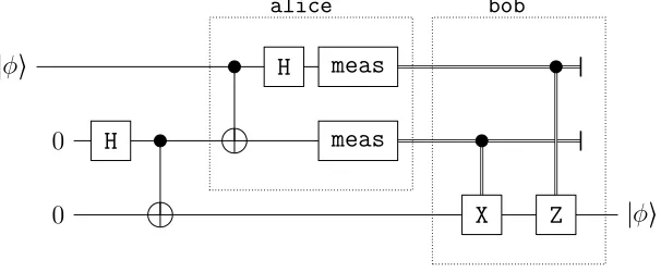
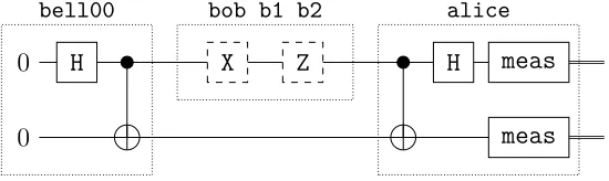
∣ϕ⟩
0
0 ∣ϕ⟩
bell00
H
alice
H meas
meas
bob
X Z
Figure 2.1: A quantum teleportation circuit
being applied to those wires.
Figure 2.1 shows the teleportation protocol from the previous section as a circuit. We explicitly initialize the bell pair √1
2∣00⟩+ 1 √
2∣11⟩ in the part of the circuit labeled
“bell00”. The CNOT gate is given a special representation as a NOT (the ⊕ on the bottom wire) “controlled” by the circle on the middle wire. Note that other gates can be controlled as well, as in the gates in the segment labeled “bob.” Alice applies a CNOT from the qubit to be transmitted to her member of the Bell pair, then applies a Hadamard and measures both qubits. We represent the output of this measurement using double lines, which represent classical bits. Bob uses these bits to control whether he applies X and Z, thereby obtaining the state of Alice’s original qubit.
2.4
Quantum States as Vectors
The exposition in the previous sections is somewhat lacking: It gives us a sense of what a quantum state is, but it does not describe what operations are quantum-mechanically valid, aside from the few operations given. To get a better sense of what operations are possible, we will switch to vector notation.
For a single qubit, the vector corresponding to α∣0⟩+β∣1⟩ is
(αβ)
.
For the more general quantum state α0∣00. . .0⟩+α1∣00. . .1⟩+ ⋅ ⋅ ⋅ +αn−1∣11. . .1⟩ we have the following vector:
⎛ ⎜⎜ ⎜ ⎝
α0 α1 ⋮ αn−1
.
Note that the kth element in the matrix is the coefficient of ∣kb⟩, where kb is the binary representation of k. This makes it easy to switch between representations.
What is the meaning of ∣ϕ⟩⊗∣ψ⟩ in vector notation? The tensor, or Kronecker product, takes an m×n matrix A and o×p matrix B and returns a mo×np matrix with copies of B tiled inside A. Visually, we have:
⎛ ⎜⎜ ⎜⎜ ⎜⎜ ⎜⎜ ⎜⎜ ⎜⎜ ⎜⎜ ⎜ ⎝
A1,1B1,1 . . . A1,1B1,p . . . . A1,nB1,1 . . . A1,nB1,p
⋮ ⋱ ⋮ . . . . ⋮ ⋱ ⋮
A1,1Bo,1 . . . A1,1Bo,p . . . . A1,nB1,1 . . . A1,nBo,p
⋮ ⋮ ⋮ ⋮ ⋮ ⋮ ⋮ ⋮
⋮ ⋮ ⋮ ⋮ ⋮ ⋮ ⋮ ⋮
⋮ ⋮ ⋮ ⋮ ⋮ ⋮ ⋮ ⋮
Am,1B1,1 . . . Am,1B1,p . . . Am,nB1,1 . . . Am,nB1,p
⋮ ⋱ ⋮ . . . . ⋮ ⋱ ⋮
Am,1Bo,1 . . . Am,1Bo,p . . . Am,nB1,1 . . . Am,nBo,p
⎞ ⎟⎟ ⎟⎟ ⎟⎟ ⎟⎟ ⎟⎟ ⎟⎟ ⎟⎟ ⎟ ⎠
Note that in the vector case, multiplying anmlength vector by ann length vector returns a vector of length mn. However, the general case of the Kronecker product will prove useful, as we will see shortly.
Exercise 4. Write(α∣0⟩+β∣1⟩)⊗(γ∣0⟩+δ∣1⟩)as a vector, first by taking the Kronecker product directly and then by simplifying the expression and transforming it into vector notation. Confirm that both results are equal.
2.4.1
Unitary transformations
What kind of operations are valid on quantum states? Let us begin by noting that quantum states ∣ϕ⟩ correspond to unit vectors, or vectors of norm 1:
∥∣ϕ⟩∥=
√ ∣α1∣
2
+ ⋅ ⋅ ⋅ +∣αn∣ 2
=1.
A valid quantum operation should preserve this property and the size of the vector. We call such operationsunitary.
Unitary transformations correspond precisely tounitary matrices, square matrices U satisfying the following:
U U†=I =U†U
the transpose of Wolfgang Pauli’s Y matrix:
Y†=(0 −i i 0)
†
=(−0 i
i 0)=( 0 −i
i 0)=Y
We see that Y happens to be its own adjoint.
Let us now multiply Y by its adjoint to confirm that it is unitary:
(0i −0i) (0i −0i)=(0+0(+−0i)i i(−0i+)0+0)=(1 00 1)
Theorem 1. For any unitary matrix U and unit vector ϕ, ∥U∣ϕ⟩∥=1
Proof. The norm of∣ϕ⟩can be represented as the product of∣ϕ⟩† and∣ϕ⟩, also written
⟨ϕ∣ ∣ϕ⟩. Technically, this is a1×1matrix, but it is isomorphic to a scalar. We call the adjoint matrix ⟨ϕ∣ abra and ∣ϕ⟩ a ket. Hence the norm of U∣ϕ⟩ can be written as
∥U∣ϕ⟩∥=(U∣ϕ⟩)†(U∣ϕ⟩) =⟨ϕ∣U†U∣ϕ⟩ =⟨ϕ∣ ∣ϕ⟩ =1
Here are the matrix forms of the operators H, X, and Z:
H= √1 2(
1 1
1 −1), X =( 0 1
1 0), Z =( 1 0 0 −1)
The controlled version of any n-qubit gate U is represented by the block matrix
( I2n 0 0 U )
The CNOT is simply the controlledX gate, and the controlled CNOT is called the Toffoli (TOF or CCNOT) gate.
Exercise 5. Note that H, X, Z, and CNOT are all their own adjoints. Verify that
these matrices are unitary.
Exercise 6. Show that H, X, Z, and CNOT have the behavior described in the
previous section. That is, show that when applied to basis vectors (1
0) and (01)they
produce the claimed output.
qubit system. We pad H on either side with 2×2 identity matrices and then apply I2⊗H⊗I2 to the quantum state. An arithmetic identity called the Kronecker mixed product says that (A⊗B)(C⊗D)=AC⊗BD (provided the dimensions line up), so if the target system is separable into ∣ψ⟩1∣ϕ⟩ ∣ψ⟩2, we get
(I2⊗H⊗I2)(∣ψ⟩1∣ϕ⟩ ∣ψ⟩2)=(I2∣ψ⟩1)⊗(H∣ψ⟩)⊗(I2∣ψ⟩2) =∣ψ⟩1(H∣ψ⟩) ∣ψ⟩2
as we would hope.
In general, a quantum computer can be expected to implement some number of unitary operations as primitive gates, though the precise set of primitives will differ based on architecture. It is important, however, that the implemented set be
universalfor quantum computation – that is, it can be used to efficiently approximate any unitary transformation. Here, the following two theorems are relevant:
Theorem 2 (Solovay-Kitaev). If a given set of gates can approximate any 2×2
unitary matrix, it can approximate any such matrix efficiently (with a sequence of gates of length log3.97(1/ϵ) where ϵ is the allowed error).
Theorem 3 (Shi (2003)). Any unitary transformation U on n qubits can be
approx-imated using Hadamard and Toffoli gates or CNOT and any single qubit gate g such that g2≠I.
The Solovay-Kitaev1 theorem (Dawson and Nielsen, 2005; Nielsen and Chuang, 2010), which was generalized to multiple qubit matrices, tells us that universal gate sets can generally be interchanged with little loss of efficiency, provided that they consist of gates on small numbers of qubits. Hence, the specific choice of gate set is likely to depend on a given quantum computer’s hardware. Shi (2003) gives a number of strong candidates for universal sets to use in practice; Aharonov (2003) discusses the variety of gate sets known to be universal.
Many functions do not correspond to valid unitary transformation and therefore cannot be applied to quantum states. One important such function is the subject of the no-cloning theorem:
Theorem 4 (No Cloning). There is no unitary transformation that copies the state
of an arbitrary qubit (that is, takes ∣ϕ⟩ ∣0⟩ to ∣ϕ⟩ ∣ϕ⟩).
This theorem is due to Dieks (1982) and Wooters and Zurek (1982); a succinct proof is given on page 523 of Nielsen and Chuang (2010). The no-cloning theorem will motivate our use of linear types (which prevent us from copying terms) in the
Qwire quantum circuit language (Chapter 4).
2.5
Mixed States as Density Matrices
At this point, we want to expand our notion of quantum states. So far, a quantum state has simply been a 2n-length complex vector, whose norm is equal to one. From here on we will call this a pure state. Note, however, that one of our operations— measurement—takes a pure state to a distribution over pure states. Since we would like to talk about these distributions directly, we will refer to them as mixed states.
Consider what happens if we apply a HadamardH to the basis state ∣0⟩and then measure it. We will obtain a distribution over∣0⟩and ∣1⟩, with 1
2 probability assigned
to each outcome. We can (naively) write this as
{ (1
2,∣0⟩), ( 1 2,∣1⟩) }
where the real numbers on the left represent probabilities and the quantum states on the right represent measurement outcomes.
What if, without looking at the outcome of the measurement, we then apply another Hadamard to the state? We should obtain
{ (1
2, H∣0⟩), ( 1
2, H∣1⟩) }
which expands out to
{ (1
2, 1
√
2∣0⟩+ 1
√
2∣1⟩), ( 1 2,
1
√
2∣0⟩− 1
√
2∣1⟩ }.
An interesting theorem of quantum mechanics says that the two distributions mentioned above are physically indistinguishable. For instance, if we measured either of the distributions above and examined the outcome, we would obtain∣0⟩with prob-ability 1
2 and ∣1⟩ with probability 1
2. If we applied a Hadamard to either state, we
would simply toggle between the two indistinguishable states, since HH∣0⟩=∣0⟩ and likewise for ∣1⟩. Ideally, any language for talking about these states would identify them, but here the language of probability distributions over quantum states fails us. Instead, we present an alternative way of representing quantum states that iden-tifies these distributions with each other. A density matrix is a square matrix of dimensions2n×2n that we can use to represent both pure and mixed quantum states. We can convert a pure state∣ϕ⟩in vector form to its density matrix representation by multiplying it by its adjoint, commonly written ⟨ϕ∣. So, for instance, the basis states
∣0⟩and ∣1⟩ become
∣0⟩ ⟨0∣=(1
0) (1 0)=( 1 0 0 0)
and
∣1⟩ ⟨1∣=(0
Conveniently, we can check if a density matrix corresponds to a pure state by squaring it. For any pure state ρ in density matrix form, ρ2=ρ, and this is true only
of pure states.
Exercise 7. Prove the first half of the above statement.
What if we want to apply a unitary matrix U to some quantum state ρ in its density matrix form? Let us first consider the case in which ρ=∣ϕ⟩ ⟨ϕ∣ (that is, ρ is a pure state). ApplyingU to∣ϕ⟩ ⟨ϕ∣should give us(U∣ϕ⟩)(U∣ϕ⟩)†. We can distribute the adjoint over multiplication, obtaining(U∣ϕ⟩)(∣ϕ⟩†U†), which we write asU∣ϕ⟩ ⟨ϕ∣U†. This gives us the formula for applying a unitary to a density matrix: We multiply the matrix by U on its left and U† on its right. Since density matrices and unitary operators are always square, if the dimensions are correct on the left, they will match up on the right.
What about measurement? This representation has the advantage of treating mea-surement as a deterministic operation on density matrices, rather than a probabilistic operation on vectors. Measuring a single qubit can be represented as follows:
meas ρ=∣0⟩ ⟨0∣ρ∣0⟩ ⟨0∣ + ∣1⟩ ⟨1∣ρ∣1⟩ ⟨1∣
You can think of this operation as adding together the two outcomes of measure-ment. The left hand side represents the event of measuring ∣0⟩ and the right-hand side, measuring ∣1⟩.
Let us return to the example that started this section. We start with the0 qubit, represented in density matrix form as
(1 00 0).
We then apply a Hadamard operator, obtaining
1
√
2( 1 1 1 −1) (
1 0 0 0) (
1
√
2( 1 1 1 −1))=
1 2(
1 1 1 1).
We then measure the state:
(1 00 0) (1
2( 1 1 1 1)) (
1 0 0 0)+(
0 0 0 1) (
1 2(
1 1 1 1)) (
0 0 1 0)
=1 2(
1 0 0 0)+
1 2(
0 0 0 1)
=1 2(
1 0 0 1)
along the diagonal represents the probability of obtaining the corresponding basis state upon measurement (when we look at the result). Note that this was also true before we measured the state: Measurement simply removed the elements that weren’t along the main diagonal, which indicated that the qubit was in a superposition, rather than a simple distribution.
As we noted earlier, applying another Hadamard to this state doesn’t change it:
1
√
2( 1 1 1 −1) (
1 2(
1 0 0 1)) (
1
√
2( 1 1 1 −1))
=1 4(
1 1 1 −1) (
1 1 1 −1)
=1 4(
2 0 0 2)
=1 2(
1 0 0 1)
Exercise 8. Show that for a pure state in density matrix form, theith element along
the diagonal is the probability of measuring ∣i⟩.
Initializing and Discarding Qubits We’ve covered how to operate on qubits,
both by applying unitary operators and by measuring them. But how do we represent adding new qubits to a system or discarding existing qubits?
Let’s start with initialization. Adding a qubit to first position in a quantum state takes ∣ϕ⟩to ∣0⟩⊗∣ϕ⟩. This corresponds to multiplying by ∣0⟩⊗I on the left, where I is the identity matrix with the same height as the target vector. In density matrix form, this corresponds to taking (∣0⟩⊗I)ρ(⟨0∣⊗I). This takes a density matrix of dimensions 2n×2n to one with dimension2n+1×2n+1.
What about discarding a qubit? We cannot discard arbitrary qubits, because they might be entangled with the rest of the state. However, if we want to discard a ∣0⟩, we can simply reverse the operation that initializes ∣0⟩:
(⟨0∣⊗I)(∣0⟩⊗I) ∣ϕ⟩=(⟨0∣ ∣0⟩⊗I) ∣ϕ⟩=(I1⊗I) ∣ϕ⟩=∣ϕ⟩
discarding a qubit, then adding a new qubit in the measured state.
This should be sufficient to understand the semantics of quantum programs, which we will introduce in the upcoming sections.
2.6
Additional Material
In this chapter, we have tried to cover those aspects of quantum computing, and only those aspects, that are relevant to this thesis. This means that we have avoided a lot of terminology that a reader might expect to see in a paper on quantum computing. Most introductions to quantum computing will refer to Hilbert spaces, vector spaces that possess an inner product (⟨ϕ∣ ∣ψ⟩ for quantum states, often written ⟨ϕ∣ψ⟩). Infinite-dimensional Hilbert spaces are of substantial interest to quantum physicists and have additional properties; however, quantum computation only deals with the specific case of finite-dimensional complex-valued vectors.
We also never explicitly discussed interference. Interference refers to two ampli-tudes canceling one another out. We saw this when we applied a Hadamard twice and obtained 1
2∣0⟩+ 1 2∣1⟩+
1 2∣0⟩−
1
2∣1⟩ = ∣0⟩. From a physical standpoint, this is an
interesting phenomenon (how are two non-zero probability events combining to form a zero-probability event?), but from a mathematical standpoint, it’s captured in the mundane statement, “superposition behaves like addition”.
Qubits are often visualized as points on a sphere, called theBloch sphere, where the poles correspond to ∣0⟩ and ∣1⟩. Using this model, we can visualize unitary operators as rotations around the sphere. In particular, Pauli’s X, Y, and Z matrices are so named because they represent rotations around thex,y, andzaxes. For our purposes, however, the vector and matrix representations of qubits have proven more useful, and geometric discussions would complicate the picture.
Chapter 3
A Brief History of Quantum
Programming and Verification
3.1
Circuits, QRAM and Classical Control
The simplest and most influential model of quantum computation is thequantum cir-cuit model(Deutsch, 1989), in which quantum operations are represented as quantum circuits like those in Section 2.3. Unfortunately, as Knill (1996) noted, circuits alone are insufficient to describe many quantum algorithms. In particular, many quantum algorithms assume a sort of control flow in which quantum operations are executed, the results are measured, and classical computations are run on the results. This cy-cle is often repeated as many times as necessary. In response, Knill proposed a set of guidelines for writing pseudocode for quantum algorithms, revolving around the
Quantum Random Access Machine, or QRAM.
The QRAM model assumes that a quantum program has distinct sets of quantum and non-quantum (classical) registers. The quantum registers are very limited in their use: We can initialize quantum registers, apply unitary operations to them, and measure them, turning them into classical registers. The results of the measurement can then be used to perform classical computations. Implicitly, all of the quantum operations are performed on a quantum processor, while the remaining operations are performed locally, as in the following diagram:
Classical Computer
Quantum Computer quantum queries
measurement results
OpenQASM (Cross et al., 2017), and Quil (Smith et al., 2016) fairly precisely: Each has distinct registers used for quantum computation, which the controlling machine may measure and use in its computation. These “quantum assembly” languages are used in practice to run quantum computations on IBM’s 20-qubit quantum computer (the IBM Quantum Experience) and Rigetti Computing’s online Quantum Processing Units.
Knill’s pseudocode guidelines suggest that quantum registers might also be used as the guard in an IF-THEN-ELSE block, without detailing how to ensure such oper-ations are quantum mechanically valid. In “Towards a Quantum Programming Lan-guage,” Selinger (2004a) proposes a narrower model for quantum computing known asquantum data, classical control. This widely adopted model states that the control flow of a quantum program should always be classical: Though we take advantage of the superposition of data, such as qubits, we should not attempt to run superpo-sitions of programs. Instead, a quantum program should use classical conditionals, loops, and recursion. Most of the languages discussed below follow this framework, with the exception of QML (Altenkirch and Grattage, 2005). We will discuss the alternative approach, known asquantum control, in Section 3.9.
So far, we’ve portrayed the interaction between classical and quantum processors as unidirectional: The classical processor sends operations to the quantum computer, which returns measurement results. However, this doesn’t tell the whole story. Occa-sionally, a quantum computation will itself depend upon some complicated classical computation, which we wouldn’t want to run on a dedicated quantum processor. This classical computation, in turn, might depend on some measurement results. To deal with this, Green et al. (2013a) introduce the notion ofdynamic lifting. This operation is initialized by the quantum processor, which sends data to the classical processor and asks it to compute the remainder of the quantum operation (in Quipper’s case, a circuit) for the QRAM to execute.
Classical Computer
Quantum Computer classical queries
circuit continuations
Many of the languages we will look at implement some form of dynamic lifting.
3.2
QCL: A General Purpose Quantum Language
follow. His QCL, an imperative-style language, included support for advanced features like management of scratch qubits (or ancillae) and automatic circuit reversal.
QCL adheres pretty closely to Knill’s (1996) guidelines for quantum programming languages. It assumes that execution of a quantum program is primarily guided by a classical computer, which has an attached QRAM device for quantum operations.
In QCL, quantum operations are applied to sets of quantum registers. There are various restricted forms of registers that allow for constant-valued qubits or registers used exclusively for scratch space. These quscratch registers are garbage-collected by a procedure that returns them to the ∣0⟩ state using Bennett’s (1973) technique. We discuss this technique in detail in Chapter 8.
QCL also allows for a sort of quantum conditional. We can annotate any function with the keywordcondto control all of its operations by a control qubit provided as an argument. This necessarily restricts the function being controlled—it must correspond to a unitary transformation on all its qubits; moreover, it cannot reference the control qubit itself. This is accomplished via strict scoping rules. This construction is then extended to allow for a limited quantum if statement and a bounded quantum while loop.
Even more so than Knill (1996), QCL established a baseline for what quantum programming languages should be able to do as well as a yardstick against which other languages could compare themselves (see, for instance, Rüdiger (2006); Green et al. (2013a)).
3.3
QPL: Semantics for Quantum Programming
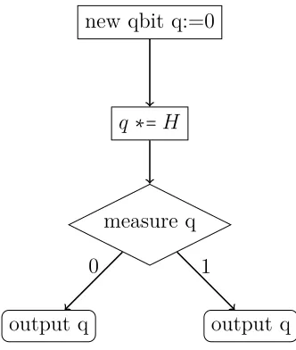
Selinger (2004a) introduced QPL (also called QFC, for Quantum Flowchart Lan-guage), the first quantum programming language with a well-defined denotational semantics, including a semantics for recursion given in terms of least-fixpoints. QPL is a flowchart language: The primary representation of a QPL program is a directed graph with branching corresponding to conditional statements (cycles correspond to loops). QPL also has a more standard representation as a functional programming language with an imperative-style syntax. That is, while it is written in an imper-ative style, it has no notion of state and its only side-effects are measurement and non-termination.
new qbit q:=0
q∗=H
measure q
output q output q
0 1
Figure 3.1: A QPL program for tossing a quantum coin
the number of bits and qubits, respectively, by treating bits as simply qubits that are always in one of the basis states. This representation is rejected in the paper in favor of economy ofrepresentation, since large sparse matrices take up a lot of space, but it is more conceptually parsimonious (easy to explain and reason about) and was adopted as the semantics for QPL by Kakutani (2009).
QPL syntax prohibits cloning qubits: While QCL and other languages fail at runtime if the user attempts to use the same qubit as both arguments to a CNOT gate, QPL doesn’t allow aliasing and can therefore check that the arguments are distinct at compile time.
While representing circuits as flowcharts didn’t catch on among quantum pro-gramming languages, QPL conveyed some important ideas that gained wide currency. Instead of including a quantum analogue of the IF statement, QPL treats measure-ment itself as a branching construct, as can be easily seen in Figure 3.1. QPL was also adopted as a target for verification efforts: Kakutani’s (2009) quantum Hoare logic QHL reasons about QPL programs, and QPL programs are given a weakest pre-expectation semantics by D’Hondt and Panangaden (2006). D’Hondt and Panan-gaden’s WP semantics is dual to the given semantics for QPL and was used in a subsequent line of work on quantum logics (Ying, 2011; Ying et al., 2017; Li and Ying, 2018).
areas of denotational semantics for quantum programs and compile time restrictions on cloning qubits. This work would form the basis for the quantum lambda calculi.
3.4
Linearity and the Quantum Lambda Calculi
Unlike in classical computation, where Alan Turing’s eponymous machines (1937) and Church’s lambda calculus (1936b) were invented simultaneously, David Deutsch’s quantum Turing machine (Deutsch, 1985) is widely considered the “founding paper” of quantum computing (though Feynman (1982), Benioff (1980), and Albert (1983) presaged it). The more popular quantum circuit model was also introduced by Deutsch (1989); Yao (1993) would demonstrate the two models’ equivalence. Quantum versions of the lambda calculus would follow, beginning with van Tonder’s (2004) λq.
λqattempts to address four issues with mixing classical and quantum computation:
1. reversibility of computation,
2. linearity of quantum states,
3. equational reasoning, and
4. completeness, or equivalence to the quantum Turing machine model.
All quantum computations must necessarily correspond to reversible functions. Unfortunately, many terms in the lambda calculus reduce to the same value, making it impossible to recover the original input (thereby making the computation irreversible and quantum mechanically impossible). Van Tonder addresses this by modifying the reduction rules in his calculus so that every reduction rule leaves a history, which allows us to recover the original lambda term.
The calculus also deals with linearity by introducing two kinds of lambda abstrac-tions:λx.ttakes a linear variable to some expressiont, in whichxmust appear exactly once. By contrast, λ!x.t may usex non-linearly and hence may only be applied to a non-linear term. Since λq has no type system, a non-linear lambda applied to a linear term is simply stuck.
Van Tonder defines an equational proof system forλq, allowing us to reason about the equivalence ofλq expressions. He also sketches a proof of equivalence between the lambda calculus and Deutsch’s quantum Turing machine. In one direction, he shows that a quantum TM can simulate the reduction of a λq expression; in the other, he shows that λq can express arbitrary quantum circuits, which Yao (1993) showed to be equivalent to quantum Turing machines.
∣ϕ⟩
0
0 ∣ϕ⟩
H
alice
H meas
meas
bob
X Z
Figure 3.2: The teleportation function, composed of the entangled functions “alice” and “bob”
Selinger and Valiron’s (2006; 2008; 2009) Quantum Lambda Calculus is primarily concerned withquantum functionsand linear type systems for typing these functions. To get a sense for quantum functions, let’s take another look at the teleport circuit (Figure 3.2). Normally we would think of the alice circuit as a function from two qubits to two bits, and we would think of bob as a function from a qubit and two bits to a qubit. But this isn’t quite accurate: Quantum teleportation only works when Alice and Bob share a pair of entangled qubits, or Bell pair, produced by the sub-circuit at the bottom left. These should be treated as a shared resource, not a separate pair of inputs. The alice function then takes a single qubit and returns a pair of bits, whilebob takes a pair of bits and returns a qubit. We can then say that for any qubit q, bob (alice q) = q. Since these two functions share entangled qubits, we call them entangled.
Another unique feature of these two quantum functions is that they’re limited in their use. The alice circuit can clearly only be used once, since it measures (and thereby destroys) its half of the Bell Pair. By contrast,bobnever measures its half, but it outputs that qubit and, hence, can no longer use it. This inspires the development of a type system to guarantee that quantum data, including quantum functions, is never duplicated.
To be precise, Selinger and Valiron’s lambda calculus incorporates an affine type system that ensures that quantum data is used at most once. This prohibits the programmer from copying data, whether in the form of qubits or quantum functions. The type system also provides a ! (bang) operator to indicate types that may be used multiple times, along with a subtyping system that allow terms of type !Ato be used wherever an A is called for. The quantum lambda calculus has an operational semantics and a categorical semantics, which are valuable but not of direct relevance to this thesis, and proofs of type soundness (progress and preservation).
lan-guage that strongly influenced both.
3.5
The Quantum IO Monad
Altenkirch and Green’s (2010) Quantum IO Monad (QIO) took some early steps towards embedding quantum computation inside a functional host language. QIO was influenced by the quantum meta-language QML (Altenkirch and Grattage, 2005), also embedded inside Haskell, but had less ambitious goals: Instead of constructing a new language that mixes quantum and classical computing (including a quantum if statement), QIO provides a monadic interface for the Haskell programmer to run quantum programs. Treating quantum computing as a monad has several advantages:
1. It neatly separates quantum and classical computation, preventing the pro-grammer from attempting to misuse quantum data in a classical program;
2. it gives QIO access to the full power of Haskell, including its typeclasses and libraries; and
3. it doesn’t restrict QIO to Haskell alone.
This last point was clearly illustrated by Green’s thesis (2010), which embed-ded the Quantum IO Monad inside Agda. Agda (Bove et al., 2009), like Coq, is a dependently-typed programming language that can also be used as a proof assistant. The Agda implementation of QIO uses dependent types to prevent some instances of qubit copying; for instance, applying a CNOT to the wires x and y requires a proof that x and y are distinct. However, Green embedded QIO in Agda mainly with an eye towards formal verification.
QIO includes a USem structure for representing the semantics of unitary opera-tors. This is easily defined upon the classical fragment of unitary gates—gates like X,CNOT, and CCNOT that can be expressed as functions on bits. For an arbitrary unitary gate U, it defines the semantics of U in terms of its effect on each of the basis states. Unfortunately, due to Agda’s lack of automation or a real or complex number library (the author wrote a small axiomatic library of his own), it proved difficult to prove that unitaries are, in fact, unitary, or to prove any properties of quantum cir-cuits. Nevertheless, QIO presaged our own efforts in this area and influenced Quipper, from which we took substantial inspiration.