Testing for Contagion: a Time-Scale Decomposition

WORKING PAPER SERIES

Testing for Contagion:

a Time-Scale Decomposition

Andrea Cipollini and Iolanda Lo Cascio

Working Paper 47

June 2010

Testing for Contagion: a Time-Scale Decomposition

Department of Economics Faculty of Economics

University of Modena and Reggio Emilia Iolanda LO CASCIO

Department of Economics, Business and Finance Faculty of Economics

University of Palermo

Abstract

The aim of the paper is to test for financial contagion by estimating a simultaneous equa-tion model subject to structural breaks. For this purpose, we use the Maximum Overlapping Discrete Wavelet Transform, MODWT, to decompose the covariance matrix of four asset returns on a scale by scale basis. This decomposition will enable us to identify the structural form model and to test for spillover effects between country specific shocks during a crisis pe-riod. We distinguish between the case of the structural form model with a single dummy and the one with multiple dummies capturing shifts in the co-movement of asset returns occur-ring duoccur-ring periods of financial turmoil. The empirical results for four East Asian emerging stock markets show that, once we account for interdependence through an (unobservable) common factor, there is hardly any evidence of contagion during the 1997-1998 financial turbulence.

1

Introduction

Since the early nineties, the international financial crises have shown that financial shocks in one country can have rapid and large impact on other countries. The literature has investigated whether the diffusion of a shock from one country to other countries can be classiffied as conta-gion. For this purpose, in this paper, we use the definition of ”shift-contagion” given by Forbes and Rigobon (2002), which interprets contagion as a significant and temporary increase in cross-market linkages after a country specific shock. Following the method developed by Forbes and Rigobon (2002), a number of studies analyze (shift) contagion via an heteroscedastic adjusted test for a correlation breakdown between asset returns. Since correlation analysis per se does not help to detect the causality direction, recently few studies interpret contagion as a temporary shift in the spillover effects of idiosyncratic shocks, once the impact of common shock/s has been filtered out. Understanding the causality direction regarding financial spillovers can help to improve the efforts for coordinated global reforms aiming at the design of the global finan-cial architecture following the most recent finanfinan-cial crises (see the study of Alexander, Eatwell, Persuad and Reoch, 2007). Few studies have acknowledged the possibility of a mutual, contem-poraneous feedback between asset returns during a crisis period. In this case, the emphasis is on

the identification of a structural form system. In order to tackle the endogeneity bias affecting the estimation of a simultaneous equation model (with structurally stable parameters), Rigobon (2003) exploits the heteroscedastic time series properties of financial time series. The identifica-tion scheme put forward by Caporale et al. (2005) and more recently by Dungey et al. (2010) relies upon structural innovations modeled through a GARCH process. The studies by Favero and Giavazzi (2002) and by Pesaran and Pick (2007) use instrumental variables (which is equiv-alent to Full Information Maximum Likelihood in case of an exactly identified system). More specifically, the method put forward by Favero and Giavazzi (2002) relies upon arbitrary zero exclusion on lagged dependent variables, while the one by Pesaran and Pick (2007) relies upon country specific exogenous regressors (hence, upon zero exclusion on exogenous variables). All these studies concentrate on the time domain. An alternative approach is proposed by Bodard and Candelon (2009) who use Granger causality test in the frequency domain. In particular, Bodard and Candelon (2009) detect contagion only in case of one market having an impact (measured via Granger causality) on another one at high frequency. In this study, we extend the analysis of Bodard and Candelon (2009) by accounting both for a potential heteroscedas-ticity bias (which, most likely, has a strong impact at high frequencies), and for an omitted variable bias (given that no common shock is included in the analysis of Bodard and Candelon, 2009). Finally, both the aforementioned time domain and the frequency domain based methods do rely on the specification of a particular dynamic model for the conditional mean, and/or for the conditional volatilities of the structural shocks. This implies that the methods described above might suffer from lag length misspecification. As an alternative to the aforementioned methods, we suggest the use of multi-scale decomposition of the reduced form covariance matrix for different asset returns. In particular, we explore the approach of Whichter et al. (2000) who use the Maximum Overlapping Discrete Wavelet Transform, MODWT, in order to com-pute the wavelet covariance and correlation on a scale by scale basis. This decomposition will enable us to disentangle the role played by the common shock and by the spillovers among idiosyncratic shocks during the financial turmoil period. In particular, we are able to identify a single dummy structural form model and, also, a multiple dummy simultaneous equation sys-tem. When focusing on the multiple dummy specification, we extend the work of Dungeyet al.

(2010) without relying on zero exclusion restrictions on the impact multiplier matrix associated with the turmoil period and by interpreting the structural form coefficients not only in terms of contagion, and hypersensitivity, but also in terms of extra-vulnerability. More specifically, while hypersensitivity is related to the vulnerability of a domestic country in crisis to shocks from other countries (see Dungey et.al (2010)), we define extra-vulnerability as the spillovers between two countries during periods of turmoil generating elsewhere (this can be motivated through portfolio-rebalancing effects). As suggested by Dungeyet al. (2010), hypersensitivity is a major concern for domestic policy makers, mainly interested in limiting the impact of foreign shocks on their own country. We argue that extra-vulnerability, as well as contagion, is a major concern for the stability of the global financial system, therefore, calling for coordinated policy makers intervention.

The empirical results show that, once we account for interdependence through an (unob-servable) common factor,we find hardly any evidence of contagion. The structure of the paper is as follows. Section 2 describes the empirical methodology, Section 3 discusses the empirical evidence and Section 4 concludes. A detailed description of wavelet analysis and of the scale by scale variance-covariance decomposition is presented in the Appendix.

2

Empirical Methodology

In this section we describe the identification method of a simultaneous equation system subject either to a single regime shift or to a multiple regime shift.

2.1 Single Dummy Specification

In line with Pesaran and Pick (2007), we allow for a potential simultaneity bias arising only during the crisis period. More specifically, we consider the following structural model to describe the joint dynamics of four East Asian stock markets (Hong Kong, Thailand, Indonesia, South Korea):

[(1−dc,t) +dc,tA]yt= Γzt+ut (1)

where dc is the realisation of a dummy variable, taking value 1 during the crisis period and

zero otherwise. From (1) we can observe that the co-movement (interdependence) between the endogenous variables entering the 4×1 column vector y, during a tranquil period is captured through the loadings coefficients entering the 4×1 matrix Γ associated with the (unobservable) common shock z_t. During the crisis period, there is a shift in the degree of co-movement between the endogenous variables due to the simultaneous spillover effects of the idiosyncratic shocks entering the 4×1 column vectoru. The impact multiplier matrix is:

A=      1 −α₁₂ −α₁₃ −α₁₄ −α21 1 −α23 −α24 −α31 −α32 1 −α33 −α₄₁ −α₄₂ −α₄₃ 1      (2)

From the simultaneous equation system in (1), we obtain the reduced form disturbances vector ²t, given by [(1 −dc,t) +dcA]−1ut. The reduced form covariance matrix Σ will shift

between tranquil and crisis periods, respectively, according to the following equations:

Σnc = [Γ0σz2Γ + Ωnc] (3)

and

Σc= [(A−1)0Γ0σz2ΓA−1+ (A−1)0ΩcA−1] (4)

In (3) and (4),σ2

z, Ωncand Ωcare the variance of the common shock, the (diagonal) covariance

matrices of the idiosyncratic structural form innovations for the tranquil and the crisis period, respectively. The set of moment conditions in equation 3 and 4 should lead to identification (through heteroscedasticity), as suggested by Rigobon (2003). In particular, due to a shift of (the 4×4 matrix) Σ, we obtain ten moment conditions per regime, therefore twenty in total. The model is then not identified given that the unknowns are twenty three. More specifically, eight unknowns are the variances of the idiosyncratic structural shocks for the two periods, twelve are the α’s coefficients measuring the spillovers between the idiosyncratic shocks during the crisis period and three are the loadings of the common shock (due to a normalization to unity of one of the four loadings in Γ). Finally, the variance of the common shock, σ2_z, is set to unity.

Since the aforementioned scheme, based on switches in the second moments over time, does not identify the model in equation (1), we put forward a method of identification and esti-mation through a scale by scale decomposition of the reduced form covariance matrix. The

Discrete Wavelet Transform (DWT) and a variant of it, the Maximum Overlapping Discrete Wavelet Transform (MODWT), generate the following decomposition (up to level J) of the sample variance-covariance matrix of the four asset returns:

Σ = Σ1+ Σ2+. . .+ Σj +. . .+ ΣJ (5)

Both transforms are described in the appendix. The subscript 1 is associated with the highest frequency scale and subscript J is associated with the lowest frequency scale.

The relationship between the reduced form covariance matrix at each scale and the structural form coefficients is given as follows. From the 2nd to the Jth scale, we have:

Σj = Γ0σz2Γ + Ωj; j=2. . . ,J (6)

where Ωjis the (diagonal) covariance matrix of the structural shocks underlying the co-movement

between the two endogenous variables for levelj. As for the first scale (the one associated with the highest frequency range), we distinguish among non-crisis and crisis periods.

In particular, during the tranquil period, the reduced form covariance matrix is given by: Σ1,nc= [Γ0σz2Γ + Ω1]. (7)

The crisis period is, instead, characterized by the following reduced form covariance matrix: Σ1,c = [(A−1)0Γ0σz2ΓA−1+ (A−1)0Ω1A−1] (8)

In other words the spillover effects between idiosyncratic shocks (occurring during the crisis period) are incorporated only in the high frequency scale covariance.

The number of unknowns is 4J + 3 + 12, where 4J is the number of standard deviations for the structural idiosyncratic shocks over the J scales.As previously explained, three unknowns are the coefficients measuring the loadings of the common shock, z (the loading of z to the Hong Kong stock market has been normalized to unity). Furthermore, σ2

z is set to unity as

well. Finally, the remaining twelve coefficients are the free parameters inA, capturing spillovers among idiosyncratic shocks. Given four endogenous variables, and a single dummy describing a temporal regime shift occurring at scale 1,we are able to retrieve J + 1 variance-covariance matrices. Since ten unique elements enter each 4×4 covariance matrix, we obtain 10(J + 1) covariance equations, thereby providing an over-identified structural form model. For instance, if we use a decomposition only up to the second scale,i.e J = 2, there are 23 unknowns and 30 equations.

2.2 Multiple Dummies Model Specification

In line with the study of Dungey et al. (2010) we distinguish among four different periods of turmoil and these are: 1) the one associated with the Thai crisis in equity markets dating from 10.07.1997 to 29.08.1997; 2) the Hong Kong crisis period, from 27.10.1997 to 17.11.1997 (which is the only one considered by Forbes and Rigobon (2002), when focusing on the East Asian financial crisis); 3) the one corresponding to the Korean crisis, running from 25.11.1997 to 31.12.1997; 4) the period spanning from 01.01.1998 to 27.02.1998, corresponding to financial turmoil in Indonesia. These periods of turbulence are modeled through four different slope dummies. The model given by equation (1) is then modified as follows:

[(1− 4 X i=1 di,c,t) + 4 X i=1 di,c,tAi]yt= Γzt+ut (9)

The dummy di,c,t is capturing the crisis in country i at time t. Given that the

country-specific turmoil periods do not overlap,P4_i=1di,c,t is equal to one for each time series observation

identified as a crisis.

We show now that, similar to the case of a single dummy, a multiple dummies structural form model can be identified only through second moment switches across scales1_.

If we rely on switches in the second moments across scales, then the moment conditions are the same as those in equations 6, 7 and equation 8 is modified as follows:

Σi_1,c = [(A−_i 1)0Γ0σ_z2ΓA_i−1+ (A−_i 1)0Ω₁A−_i 1] (10)

where istands for thei-th country.

The number of unknowns is given by 4J+ 3 + 12×4, where, now, there are four different impact multiplier matrices, each with twelve free parameters and corresponding to four different crisis periods. Given four endogenous variables and four dummies, we are able to retrieveJ+ 4 variance-covariance matrices. Given ten unique elements in each 4×4 covariance matrix, we obtain 10(J + 4) covariance equations, providing an over-identified structural form model. For instance, if we use a decomposition only up to the second scale,i.eJ = 2, there are 59 unknowns and 60 equations.

We now turn to the interpretation of the off-diagonal elements of the impact multiplier matrices, which can be classified as contagion, hypersensitivity and extra-vulnerability.

Contagion, defined as the impact on the home country i during a crisis in foreign country

l, is modeled through the column l coefficients of the impact multiplier matrix associated with crisis in country l. For instance, the coefficients entering column 1 of the A₁ matrix are those picking contagion effects originating in Hong Kong. Moreover, contagion occurs only when the aforementioned parameters are positive.

Hypersensitivity (see Dungey et al. (2010)) is given by the parameters measuring the addi-tional impact of foreign shocks during a domestic crisis. Therefore, hypersensitivity is captured by the rowicoefficients of the impact multiplier matrix associated with crisis in countryi. For instance, the coefficients entering row 1 of theA₁matrix are those picking up the hypersensitivity of the Hong Kong stock market.

Finally, we interpret the remaining coefficients of the impact multiplier matrix, corresponding to each different turmoil period, as extra-vulnerability (i.e., in the case of Hong Kong all the coefficients not belonging to row and column 1 of theA1 matrix).

2.3 Estimation and Inference

An important feature of a wavelet analysis consists in the fact that it is an energy-preserving transform; as a consequence, the variance of a stochastic process is perfectly captured by the variance of the wavelet coefficients. In a similar way, the covariance between two time series is perfectly captured by the covariance of the wavelet coefficients of the two series on a scale-by-scale basis (see equation (5)). As a consequence,the orthogonality among wavelet coefficients of

1_{In case of switches in the second moments over time, the total number of equations is equal to 10×5 = 50.}

The total number of unknowns is given by 12×4 = 48 spillover effects, plus 4×5 = 20 variances of the structural shocks in addition to the 3 loadings of the common shock. Therefore, letting the covariance matrices to switch across time will not identify the structural form model.

different scales implies that the Gaussian log-likelihood can be expressed as the sum of Gaussian log-likelihood functions, each associated with a given scale covariance matrix.

Each covariance matrix is then expressed in terms of the structural form coefficients, A, Γ, Ω1, Ω2, . . . , ΩJ. The simultaneous equation model parameters with a single dummy are then

estimated by maximising the Gaussian log-likelihood:

T X t=1 h (1−dc,t)L(Γ,Ω1; ¯β1,t) +dc,tL(A,Γ,Ω1; ¯β1,t) +L(Γ,Ω2; ¯β2,t) +. . .+L(Γ,ΩJ; ¯βJ,t) i (11)

where ¯βj,t is the vector of wavelet coefficients, at scale j, produced by the MODWT applied to

the four asset returns.

The simultaneous equation model parameters with four dummies are estimated by maximising the Gaussian log-likelihood:

T X t=1 h (1− 4 X i=1 dc,t)L(Γ,Ω1; ¯β1,t) + 4 X i=1 dc,i,tL(Ai,Γ,Ω1; ¯β1,t) +L(Γ,Ω2; ¯β2,t) +. . .+L(Γ,ΩJ; ¯βJ,t) i (12)

Secondly, to make inference, we use a robust estimator of the covariance matrix of the pa-rameters estimates, given by H−10_GH−1_{, where G is the cross-product of the first derivatives}

(evaluated at the vector of parameter estimates ˆθ ), that is:

G= 1 T T X t=1 Ã ∂Lt ∂θˆ !Ã ∂Lt ∂θˆ ! (13)

Here T is the total number of observations, andH is the Hessian (evaluated at the vector of parameter estimates ˆθ): H = 1 T T X t=1 ∂2_L t ∂θ∂ˆ θˆ0 (14)

2.4 Test for Over-Identifying Restrictions

The test for the over-identifying restrictions is based upon the comparison of the (max) log-likelihood of the structural form model in equation (11) with the (max ) log-log-likelihood of the reduced form model, given by:

T X t=1

h

(1−d_c,t)L(Σ_1,nc; ¯β_1,t) +d_c,tL(Σ_1,c; ¯β_1,t) +L(Σ₂; ¯β_2,t) +. . .+L(Σ_J; ¯β_J,t)i (15)

where Σ1,c and Σ1,nc are the reduced form covariance matrices of the first-scale wavelet

coeffi-cients for the crisis and non-crisis periods respectively and Σjforj= 2. . . J are the reduced form

covariance matrices of thej−thscale wavelet coefficients. Given the orthogonality across scales, the ten parameters entering each covariance matrix Σj forj= 2, . . . , J, have been obtained by

maximising the log-likelihood

T X t=1

h

As for the parameters entering the first scale reduced form covariance matrix for the tranquil and a single financial turmoil period, we maximize the log-likelihood

T X t=1 h (1−dc,t)L(Σ1,nc; ¯β1,t) +dc,tL(Σ1,c; ¯β1,t) i (17)

As for the parameters entering the first scale reduced form covariance matrix for the tranquil and a financial turmoil period captured by four dummies, we maximize the log-likelihood

T X t=1 h (1− 4 X i=1 di,c,t)L(Σ1,nc; ¯β1,t) + 4 X i=1 di,c,tL(Σi1,c; ¯β1,t) i (18)

3

Empirical Results

We consider four East Asian emerging stock markets returns (in US dollars) computed taking the log changes in the daily US dollar-valued equity market indices for each country (multiplied by 100). The countries under investigation are Hong Kong, Korea, Thailand and Indonesia. The sample period for the asset returns (in percentages) runs from 02.01.1991 to 28.12.2007, and, after removing all the observations with zero returns, we end up with a sample of 3968 observations. For robustness we consider different levels of decomposition of the covariance matrix. In particular, in the least detailed specification, we use a two scale decomposition, and, in order to achieve finer decomposition, we use decompositions up to scale seven.

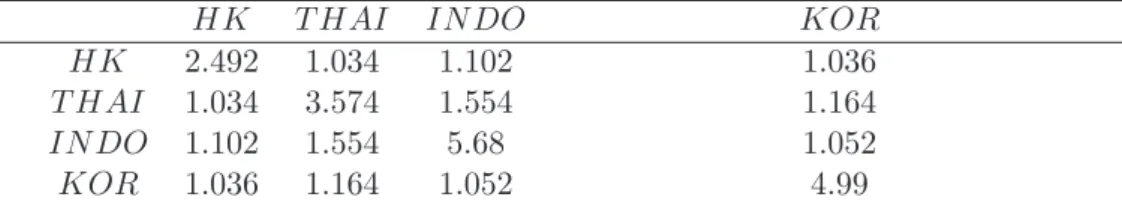
Table 1 of the appendix shows the descriptive statistics for the entire sample. Table 2a and 2b give the sample covariance matrix and its seven scale-by-scale decomposition for the full sample. We can observe that each entry in table 2a is the sum of the corresponding entries in the covariance matrices of table 2b for the seven levels of decomposition. The model described in Section 2.1 is based upon the specification of a single dummy variable taking value equal to one during the crisis period. The period of turmoil picked by a single dummy is exogenously given and it is, first, set to take values equal to one only during the Hong Kong crisis period (running from 27.10.1997to17.11.1997, as specified in the studies of Billio and Pelizzon, 2003, and of Rigobon, 2003). The other single dummy specification is set to take values equal to one during the whole East Asian turmoil period, running from 27.10.1997 to 27.02.1998, ending with the period of high volatility in returns associated with political uncertainty and IMF negotiations regarding the Indonesian crisis.

The results associated with the model based upon the specification of a dummy taking value equal to one only during the Hong Kong crisis period is given in Tables 3, 4 and 5. The empirical evidence corresponding to the model based upon the specification of a dummy taking value equal to one during the whole East Asian turmoil period, running from 27 October 1997 to 27 February 1998, are given in Tables 6,7 and 8.

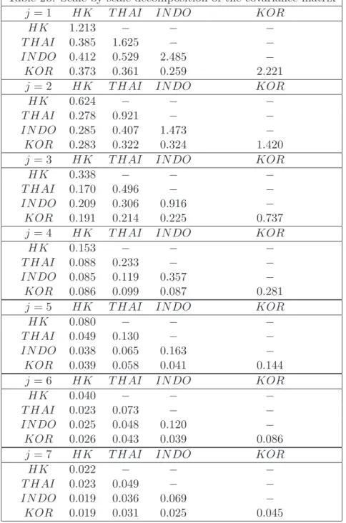
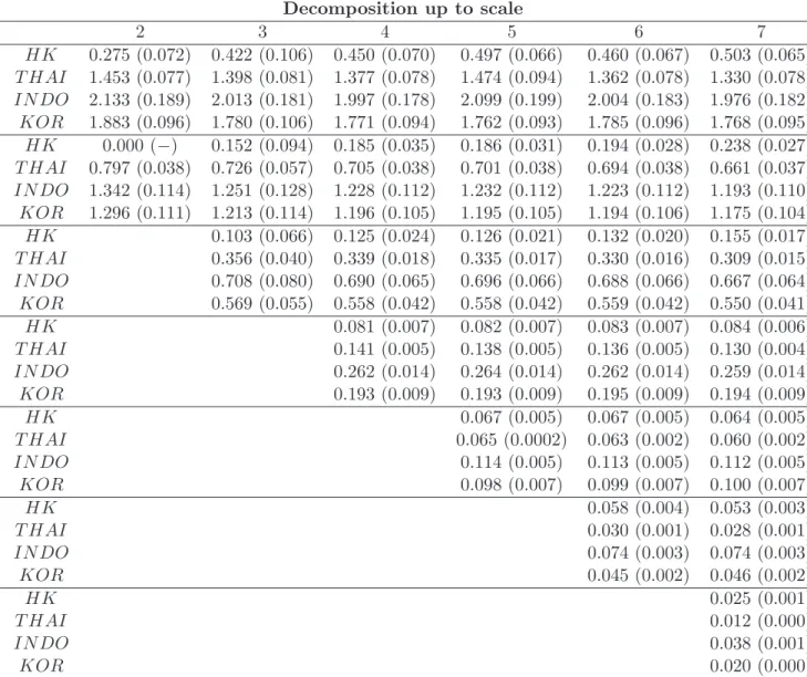
Tables 3 and 6 give the point estimates and associated standard errors for the parameters measuring the volatilities (e.g. the standard deviations) of the wavelet coefficients for different scale decompositions. The different levels of decomposition can be read along each row. For instance, the first row in Table 3 gives the volatilies associated with level 1 for levels of decompo-sition which are finer the more we move towards the last column. More specifically, the element entering the first row, first column of Table 3 is equal to 0.271 and this gives the volatility of the Hong Kong stock market for level 1 using a decomposition up to the second scale; the element entering the first row, second column of Table 3 is equal to 0.320 and this gives the volatility of the Hong Kong stock market for level 1 using a decomposition up to the third scale, and so

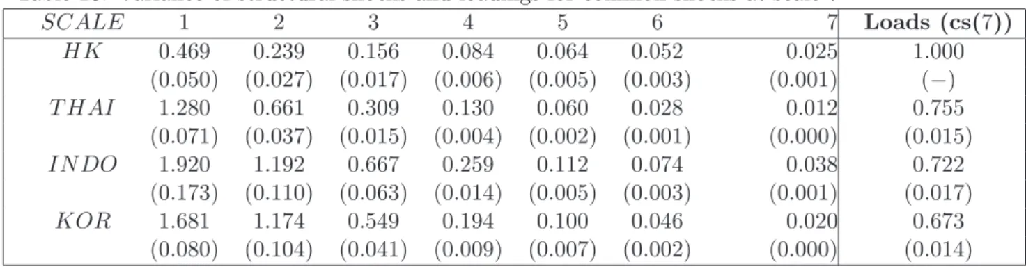
on. As we can observe from Tables 3 and 6, for each country, all the volatilities parameters are statistically significant and they differ across scales. The scale varying volatilities prove that the suggested identification scheme is supported by the empirical evidence. Furthermore, in line with the reduced form variances reported in Table 2b, the volatilities for the structural form innovations decrease (as we expect) from the scale associated with the highest frequency (that is, scale 1) the scale associated with the lowest frequency (that is, scale 7). In line with the decomposition of the reduced form variance-covariance matrix, the Indonesian stock market ex-hibits the highest volatility across all the scales, followed by the Korean, Thai e Hong Kong stock market. To be more precise, from the first to the fourth scale, the volatility of the Thai stock market is higher than the Hong Kong stock market, then, from the fifth to the seventh scale, the reverse is true. The first scale (e.g. the one associated with the highest frequency) contributes nearly 50 per cent of the overall volatility in each stock market. The volatility pattern showed in Table 3 and 6 (associated with a single dummy structural form model) and described so far is similar to the one in Table 10 (associated with a structural form model associated with four regime shifts, that is the one including four dummies), although there is a slight decrease for the size of the shock driving market turbulence (measured by the volatility coefficient at the first scale) in each country.

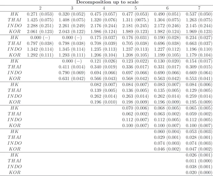
As for interdependence, we, first, want to point out the robustness of the empirical results across different scales. The point estimates and the associated standard errors for the parameters measuring the loadings of the (unobservable) common shock are given in Tables 4 and 7. These coefficients are all statistically significant and below one. If we put the emphasis on the finer level of decomposition (that is a decomposition up to level 7, as indicated in the last column of Table 4 and 7), the common factor loadings range from 0.654 to 0.756 when moving from the Korean to the Thai stock market (when we consider Table 4), whereas they range from 0.671 to 0.755 when moving from the Korean to the Thai stock market (when we concentrate on Table 7). Furthermore, we find that the finer is the variance-covariance decomposition, the higher the loadings are. Finally, given the normalization to unity for the loading of the common shock to the Hong Kong stock market, these findings suggest a higher degree of interdependence between pair of countries which do include Hong Kong.

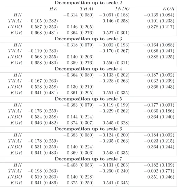
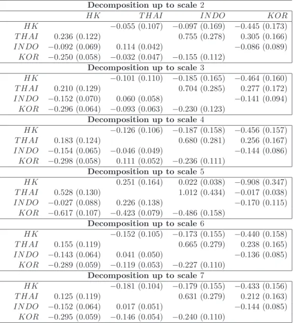
The estimation results for the spillover effects using the model with a single dummy, capturing only the turmoil associated with the crash in the Hong Kong stock market (running from 27 October 1997 to 17 November 1997) are given in Table 5. As we can observe, there is no evidence of contagion (the coefficient with positive sign are statistically insignificant) and the only statistically significant coefficients are those measuring a negative spillover effect from Korea and, especially, Thailand (e.g. the country where the financial turmoil initiated) to Hong Kong. The estimation results for the spillover effects using the model with a single dummy, capturing the longest financial turmoil period (running from 27.10.1997 to 27.02.1998) are given in Table 8. The only statistically significant positive coefficient (implying evidence of contagion) across all different level of decomposition is the one measuring the impact of Indonesia on Thailand. The remaining statistically significant coefficients are negative, and these are: a) those measuring the spillover from Hong to Korea (and also to Indonesia, if we refer to a decomposition either up to scale 4, or to scale 6 or to scale 7); b) from Thailand to Korea (if we refer to to a decomposition either up to scale 6 or to 7); c) from Indonesia to Korea;d) from Korea to Hong Kong.

In Table 9 we report the estimation results for the spillover effects using four dummies, each associated with crisis starting in one specific country. More specifically, in line with Dungey et al. (2010), the Hong Kong crisis period is set as 27 October 1997 to 17 November 1997, the Indonesian crisis period is set as 1 January 1998 to 27 February 1998, the Korean crisis runs from 25 November 1997 to 31 December 1997 and the Thai crisis in equity markets dates from

10 June 1997 to 29 August 1997. The empirical evidence confirms the findings presented in Table 5 and 8. As explained in Section 2.2, we can classify the spillovers among idiosyncratic shocks into contagion, hypersensitivity and extra vulnerability. As for the parameters measuring contagion, we find mainly evidence of negative spillovers. During the Hong Kong crisis period, a shock originating from the Hong Kong stock market has a negative effect on the Indonesian and Korean stock market. During the Korean turmoil period, a Korean stock market shock has a negative effect only on Hong Kong. During the Indonesian financial turbulence period, an Indonesian stock market shock has a negative effect on Thailand and Hong Kong, The only evidence of ”pure” contagion is captured by the positive impact of a shock originating in Korea and affecting the Thai stock market during the Korean crisis.

As for hypersensitivity, that is, the vulnerability of domestic stock market to foreign shocks during turmoil affecting the domestic country, there is mainly evidence of negative spillovers. The only positive (statistically significant) coefficient regarding hypersensitivity is the one mea-suring the reaction of the Indonesian stock market to a shock originating in the Thai stock market during the Indonesian crisis period. There is evidence of a statistically significant and negative impact effect of foreign shocks originating in Hong Kong on Korea during the Korean period of financial turbulence. There is also evidence of a statistically significant and negative impact effect of Korea on Hong Kong during turmoil affecting Hong Kong.

Evidence of what we define as extra-vulnerability mainly manifests through negative spillovers and they are given by: a) the impact of Korea on Hong Kong during the Thai crisis; b) the impact of Korea on Indonesia, of Thailand on Korea, and of Indonesia on Korea, during the Hong Kong period of financial turmoil; c) the impact of Hong Kong on Indonesia during the Korean crisis period; d) the impact of Hong Kong on Thailand and of Indonesia on Hong Kong during the Indonesian turmoil period; The few cases were extra-vulnerability manifests through positive (and statistically significant) spillovers are, first, related to the Korean period of turbulence, where there is a positive impact of Hong Kong and of Indonesia on Thailand. Finally, positive extra-vulnerability shows up during the Indonesian crisis only when considering the influence of Hong Kong on Korea.

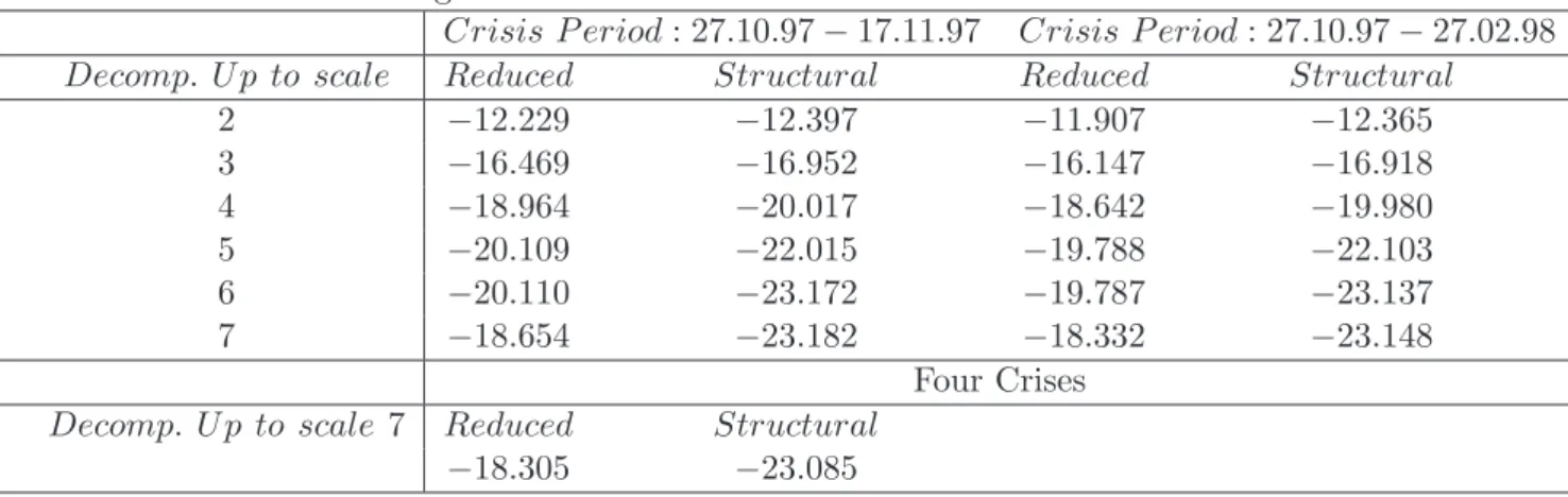
We also report in Table 10 the log-likelihood (maximum) value obtained for the reduced and structural form models associated with different scale decompositions and different crises periods. A likelihood ratio test will have asymptotically a chi square distribution with a number of degrees of freedom which, in case of a single dummy model, is equal to seven, thirteen, nineteen, twenty-five, thirty-one and thirty-seven for a level decomposition up to scale 2, 3, 4, 5, 6, or up to scale 7, respectively. Moreover, in case of the four dummies model specification, a likelihood ratio test will have asymptotically a chi square distribution with a number of degrees of freedom which is equal to one, seven, thirteen, nineteen, twenty-five and thirty-one for a level decomposition up to scale 2, 3, 4, 5, 6, or up to scale 7, respectively. As we can observe the results are robust across different model specifications, with values of the structural form very close to (and smaller than) those of the reduce form, implying p-values close to one. These findings lead us to conclude that a likelihood ratio test would accept the over-identifying restrictions.

4

Conclusions

In this paper we have used the Maximum Overlapping Discrete Wavelet Transform, MODWT, in order to decompose, on a scale by scale basis, the covariance matrix of four asset returns. We argue that this decomposition enables us to retrieve enough moment conditions necessary to identify both the loadings of the unobservable common shock (e.g. the one driving interdepen-dencies) and, more importantly, the contemporaneous spillover effects of the idiosyncratic shock

arising during a crisis period. The method proposed is particularly suitable for the identification of structural form model with multiple regime shifts (captured through deterministic dummies). An application of the proposed method to four East Asian emerging stock markets shows hardly any evidence of contagion, during the 1997-1998 period of turmoil across the region. We do find evidence of hypersensitivity and extra-vulnerability mainly manifesting through negative spillovers. We argue that the method proposed here to tackle the endogeneity bias has a number of potential interesting application, such as the identification of monetary policy shocks within a simultaneous equation model either structurally stable or subject to regime shift(s). We leave this for future research.

References

Alexander, K., Eatwell, J., Persuad, A., Reoch, R., (2007), Financial supervision and crisis management in the EU”. EU Policy Department Economic and Scientific Policy Document IP/A/ECON/IC/2007-069.

Bodard V. and B. Candelon (2009), Evidence of Contagion and Interdependence using a Fre-quency Domain Framework, Emerging Markets Review,10 140-150

Bruce, A. G. and H. Y.Gao, (1996), Understanding WaveShrink: variance and bias estimation,

Biometrika, 83,727–745.

Caporale, G., Cipollini, A., Spagnolo, N., (2005), Testing for contagion: a conditional correlation analysis,Empirical Finance,12, 476-489.

Coifman, R.R. and D.L Donoho, (1995), Translation-Invariant Denoising, in Wavelets and Statistics (Lecture Notes in Statistics, Vol.103), edited by Antoniadis A. and G. Oppenheim. New York: Springer-Verlag, 125-50.

Dungey, M., Milunovich, G. and S. Thorp, (2010) Unobservable Shocks as Carriers of Contagion,

Journal of Banking and Finance, Vol. 34, 1008-1021.

Favero and Giavazzi (2002), Is the International Propagation of Financial shocks nonlinear? Evidence from the ERM, Journal of International Economics, 57(1), 231-246.

Forbes and Rigobon (2002), No Contagion, Only Interdependence: Measuring Stock Market Co-movements, Journal of Finance,Vol. 57, No. 5, pp. 2223-61.

Grossmann, A and J. Morlet, (1984), Decomposition of Hardy functions into Square Integrable Wavelets of Constant Shape,SIAM Journal on Mathematical Analysis, 15, 723–36.

Mallat, S.G., (1987), A Compact Multiresolution Representation: The Wavelet Model, in Pro-ceedings of the IEEE Computer Society Workshop on Computer Vision, 2–7, IEEE Computer Society Press, Washington, D.C., 1987.

Nason, G.P. and B. Silverman, (1995), The Stationary Wavelet Transform and Some Statistical Applications, in Wavelets and Statistics, vol. 103 edited by A.Antoniadis and G. Oppenheim. New York: Springer-Verlag, 281–99.

Pesaran, H. and Pick A. (2007), Econometric Issues In The Analysis Of Contagion, Journal of Economic Dynamics and Control, Vol 31, Issue 4, pp. 1245-1277, 2007.

Pesquet, J.-C., Krim, H. and Carfantan H., (1996), Time-Invariant Orthonormal Wavelet Rep-resentations,IEEE Transactions on signal Processing, 44, 1964–70.

Rigobon, R. (2003), Identification through heteroscedasticity, The Review of Economics and Statistics, 2003, vol. 85, issue 4, pages 777-792

Whitcher, B.J, (1998), Assessing Non Stationary Time Series Using Wavelets, Ph.D Disserta-tion.

Whichter P. Guttorp, and D. B. Percival (2000), Wavelet Analysis of Covariance with Applica-tion to Atmospheric Time Series,Journal of Geophysical Research, 105 (D11), 14,941-14,962

A

Appendix

Wavelet analysis provides a non parametric and mathematically concise way of studying the heterogeneity of economic phenomena by analysing data over different scales, with different degree of resolution.

The term wavelet has been introduced by Grossman and Morlet (1984) to describe a square integrable function whose translation and dilation form a basis of L2_{(R), the space of all the}

square integrable functions in R. All the basis functions are self-similar, namely, they differ only by translation and change of scale from one another.

Wavelet analysis can be considered as a windowing technique with variable-sized regions. In-stead of decomposing a data sequence into sines and cosines at different frequencies–as Fourier analysis does–which do not have limited duration but extend from minus to plus infinity, a wavelet analysis decomposes it into shifted (translated) and scaled (dilated or compressed) ver-sions of amother wavelet.–ψ(t). Discontinuities in signals can be then described in terms of very short basis functions with a high-frequency content, whereas a fine analysis at low frequencies can be achieved using highly dilated basis functions.

The object of a wavelet analysis is to associate an amplitude coefficient to each of the wavelet. The task is accomplished by the Discrete Wavelet Transform which is implemented via the pyra-mid algorithm of Mallat (1987). If certain conditions are satisfied, these coefficients completely characterize the signal which is resolved in terms of a coarse approximation and the sum of fine details.

Conventional dyadic multiresolution analysis applies to a succession of frequency intervals in the form of (π/2j_{, π/2}j−1_{);j= 1,2, . . . , n, whose bandwidths are halved repeatedly descending}

from high frequencies to low frequencies. By thejthround, there will bejwavelet bands and one accompanying scaling function band. The set {ψj(t−2jk);t, k∈ I} containing T /2j mutually

orthogonal wavelets, separated from each other by 2j _{points, will be complemented by the set} {φj(t−2jk);t, k∈I} that span the lower frequency range [0, π/2j). In other words, they form

bases for the corresponding details and approximation spaces,Wj andVj respectively2.

The wavelet basis {ψ_j,k(t) = 2−j/2_ψ(2−j_{t−k);j, k ∈ I}forms an orthonormal basis in W} j.

Wj is the space containing the detail information necessary to go from an approximation with

resolution 2j−1 _{to a coarser approximation with resolution 2}j_{. Forj < n it follows that}

Vj =Vn⊕Wn⊕Wn−1⊕Wj+1 (19)

where all these subspaces are orthogonal. This implies a decomposition ofL2(R) into mutu-ally orthogonal subspaces, namely, L2_{(R) =⊕}

j∈IWj.

It turns out that, whenever a collection of closed subset satisfies the MRA definition, then, there exists an orthonormal wavelet basis {ψj,k;j, k∈ I} of L2(R), ψj,k(t) = 2−j/2ψ(2−jt−k)

such that any functionf(t)∈L2_{(R) can be represented as a sequence of projections onto father}

(scaling) and mother (wavelets) functions, namely:

f(t) =X k γJ,kφJ,k(t) + X j X k βj,kψj,k (20)

J is the highest possible level of decomposition andγj,k andβj,k are the following projections

of f(t) on the bases φj,k and ψj,k respectively:

γ_j,k = Z f(t)φ_j,k(t)dt βj,k = Z f(t)ψj,k(t)dt (21)

The signal can then be written as a set of orthogonal components at resolutions 1 to J:

f(t) =SJ+DJ +DJ−1+. . .+D1 (22)

An important feature of a wavelet analysis consists in the fact that it is an energy-preserving transform; as a consequence, the variance of the signal is perfectly captured by the variance of the coefficients. In other words, the overall variance of the data can be expressed as a sum of the variances within the frequency bands, which may be indexed by j:

σ2 = ∞ X j=1 σ_j2 (23) whereσ2

j is the contribution of the variability at scale 2−jto the overall variability of the process:

σ_j2 = 1

2jV ar(βj,t) (24)

As with the wavelet variance for univariate processes, the wavelet covariance decomposes the covariance between two stochastic processes on a scale-by-scale basis (Whitcher,1998). For a bivariate stochastic process Xt= (x1,t, x2,t), there will be:

∞ X j=1 CovX(j) =Cov(x1,t, x2,t) (25) where CovX(j) = 1 2jCov(β1,j,t, β2,j,t) (26)

A disadvantage of the conventional dyadic wavelet analysis is the restriction on the sample sizeT which has to be a power of 2. A further problem lies in the fact that the DWT depends upon a non-symmetric filter that is liable to induce a phase lag in the processed data.

The Maximum Overlapping Discrete Wavelet Transform (MODWT) (known under many different names, i.e., Stationary Wavelet Transform (Nason and Silverman, 1995), Translation Invariant DWT (Coifman and Donoho, 1995), Time Invariant DWT (Pesquet et al. 1996),

Non-Decimated DWT (Bruce and Gao, 1996)) represents an attempt to generate a transform that is not sensitive to the choice of the starting point for the data series. In order to avoid such sensitivity, the filtered output at each stage of the pyramid algorithm is not subjected to downsampling. As a consequence, the number of coefficients generated at the jth stage of the decomposition are in number equal to the sample size, T, instead that equal to T /2j.

An important feature of the MODWT is that, besides handling any sample size, the detail and smooth coefficients of the multiresolution analysis are associated with linear phase filters. The consequence is that it is possible to align the features of the original time series with those of the multiresolution analysis.

An unbiased estimator of the wavelet variance is based on the ˜Nj =N−Lj+ 1 non boundary

coefficients (those coefficients that are unaffected by circularity)34 _{produced by the MODWT.}

3_{The DWT, as well as its variants, the Partial DWT and the MODWT, makes use of circular filtering.}

The series under investigation is treated as if it is a portion of a periodic sequence with period N. In other words,the transform considers XN−1, XN−2. . . as useful surrogates for the unobservedX−1, X−2, . . .. This can

be a questionable assumption for some time series. The effects of this assumption, and solutions to the problems created, are fully explored in Perciwal and Walden (2000).

4_L

Table 1: Descriptive Statistics (Sample period: 02.01.1991– 28.12.2007) HK T HAI IN DO KOR M ean 0.000 0.000 0.000 0.000 M ax 17.25 15.40 23.00 26.32 M in −14.70 15.84 −40.55 −21.44 Std dev 1.58 1.89 2.38 2.23 JB p−value 0.000 0.000 0.000 0.000

Table 2a: Sample covariance matrix (Sample period: 02.01.1991– 28.12.2007)

HK T HAI IN DO KOR

HK 2.492 1.034 1.102 1.036

T HAI 1.034 3.574 1.554 1.164

IN DO 1.102 1.554 5.68 1.052

Table 2b: Scale-by-scale decomposition of the covariance matrix j = 1 HK T HAI IN DO KOR HK 1.213 − − − T HAI 0.385 1.625 − − IN DO 0.412 0.529 2.485 − KOR 0.373 0.361 0.259 2.221 j = 2 HK T HAI IN DO KOR HK 0.624 − − − T HAI 0.278 0.921 − − IN DO 0.285 0.407 1.473 − KOR 0.283 0.322 0.324 1.420 j = 3 HK T HAI IN DO KOR HK 0.338 − − − T HAI 0.170 0.496 − − IN DO 0.209 0.306 0.916 − KOR 0.191 0.214 0.225 0.737 j = 4 HK T HAI IN DO KOR HK 0.153 − − − T HAI 0.088 0.233 − − IN DO 0.085 0.119 0.357 − KOR 0.086 0.099 0.087 0.281 j = 5 HK T HAI IN DO KOR HK 0.080 − − − T HAI 0.049 0.130 − − IN DO 0.038 0.065 0.163 − KOR 0.039 0.058 0.041 0.144 j = 6 HK T HAI IN DO KOR HK 0.040 − − − T HAI 0.023 0.073 − − IN DO 0.025 0.048 0.120 − KOR 0.026 0.043 0.039 0.086 j = 7 HK T HAI IN DO KOR HK 0.022 − − − T HAI 0.023 0.049 − − IN DO 0.019 0.036 0.069 − KOR 0.019 0.031 0.025 0.045

Table 3: Variances of structural shocks (Crisis period:27.10.1997-17.11.1997 (Hong Kong crisis)) Decomposition up to scale 2 3 4 5 6 7 HK 0.271 (0.053) 0.320 (0.052) 0.475 (0.057) 0.477 (0.053) 0.490 (0.051) 0.537 (0.050) T HAI 1.425 (0.075) 1.408 (0.075) 1.320 (0.076) 1.311 (0075.) 1.304 (0.075) 1.263 (0.075) IN DO 2.288 (0.251) 2.261 (0.249) 2.176 (0.244) 2.181 (0.245) 2.172 (0.246) 2.145 (0.244) KOR 2.061 (0.123) 2.043 (0.122) 1.986 (0.124) 1.989 (0.123) 1.982 (0.124) 1.969 (0.123) HK 0.000 (−) 0.000 (−) 0.175 (0.037) 0.176 (0.031) 0.190 (0.028) 0.234 (0.027) T HAI 0.797 (0.038) 0.798 (0.038) 0.708 (0.039) 0.705 (0.038) 0.696 (0.038) 0.663 (0.037) IN DO 1.342 (0.114) 1.345 (0.114) 1.235 (0.113) 1.237 (0.113) 1.227 (0.112) 1.196 (0.110) KOR 1.292 (0.111) 1.293 (0.111) 1.206 (0.104) 1.208 (0.105) 1.199 (0.105) 1.179 (0.104) HK 0.000 (−) 0.121 (0.026) 0.123 (0.022) 0.130 (0.020) 0.154 (0.017) T HAI 0.411 (0.014) 0.340 (0.019) 0.336 (0.017) 0.331 (0.017) 0.309 (0.015) IN DO 0.790 (0.069) 0.694 (0.066) 0.697 (0.066) 0.690 (0.066) 0.669 (0.064) KOR 0.631 (0.042) 0.566 (0.043) 0.568 (0.042) 0.563 (0.042) 0.553 (0.041) HK 0.082 (0.007) 0.084 (0.007) 0.083 (0.007) 0.084 (0.006) T HAI 0.139 (0.005) 0.136 (0.005) 0.135 (0.005) 0.129 (0.005) IN DO 0.262 (0.014) 0.263 (0.014) 0.262 (0.014) 0.259 (0.014) KOR 0.196 (0.010) 0.198 (0.009) 0.196 (0.009) 0.195 (0.009) HK 0.070 (0.006) 0.068 (0.005) 0.065 (0.005) T HAI 0.062 (0.002) 0.063 (0.002) 0.059 (0.002) IN DO 0.112 (0.007) 0.112 (0.005) 0.112 (0.005) KOR 0.100 (0.007) 0.100 (0.007) 0.100 (0.007) HK 0.060 (0.004) 0.053 (0.003) T HAI 0.029 (0.001) 0.028 (0.001) IN DO 0.074 (0.003) 0.074 (0.003) KOR 0.046 (0.002) 0.047 (0.002) HK 0.026 (0.001) T HAI 0.011 (0.000) IN DO 0.038 (0.001) KOR 0.020 (0.000)

Table 4: Loadings for the common shock (Crisis period: 27.10.1997-17.11.1997 (Hong Kong crisis)

Decomposition up to scale 2 3 4 5 6 7 HK − − − − − − T HAI 0.458 (0.028) 0.482 (0.023) 0.642 (0.028) 0.673 (0.020) 0.682 (0.017) 0.756 (0.014) IN DO 0.455 (0.037) 0.521 (0.033) 0.682 (0.040) 0.657 (0.028) 0.675 (0.021) 0.714 (0.017) KOR 0.434 (0.033) 0.493 (0.025) 0.627 (0.027) 0.607 (0.020) 0.628 (0.015) 0.654 (0.014)

Table 5: Spillover effects( Crisis period: 27.10.1997-17.11.1997 (Hong Kong crisis)) Decomposition up to scale 2 HK T HAI IN DO KOR HK −0.314 (0.080) −0.061 (0.188) −0.139 (0.084) T HAI −0.105 (0.282) −0.146 (0.258) 0.101 (0.233) IN DO 0.587 (0.353) 0.146 (0.205) 0.378 (0.217) KOR 0.668 (0.481) 0.364 (0.276) 0.527 (0.301) Decomposition up to scale 3 HK −0.318 (0.079) −0.092 (0.193) −0.164 (0.088) T HAI −0.119 (0.280) −0.170 (0.267) 0.086 (0.241) IN DO 0.568 (0.355) 0.140 (0.206) 0.388 (0.225) KOR 0.658 (0.480) 0.359 (0.276) 0.550 (0.311) Decomposition up to scale 4 HK −0.364 (0.080) −0.133 (0.202) −0.187 (0.092) T HAI −0.167 (0.263) −0.228 (0.263) 0.032 (0.239) IN DO 0.528 (0.358) 0.130 (0.219) 0.366 (0.243) KOR 0.641 (0.481) 0.361 (0.295) 0.551 (0.335) Decomposition up to scale 5 HK −0.383 (0.079) −0.119 (0.199) −0.177 (0.091) T HAI −0.176 (0.259) −0.229 (0.262) −0.030 (0.186) IN DO 0.534 (0.358) 0.144 (0.224) 0.364 (0.240) KOR 0.646 (0.482) 0.374 (0.307) 0.545 (0.328) Decomposition up to scale 6 HK −0.383 (0.080) −0.124 (0.200) −0.184 (0.092) T HAI −0.178 (0.259) −0.235 (0.263) −0.023 (0.215) IN DO 0.531 (0.359) 0.140 (0.224) 0.364 (0.244) KOR 0.641 (0.483) 0.369 (0.306) 0.543 (0.335) Decomposition up to scale 7 HK −0.408 (0.083) −0.131 (0.203) −0.182 (0.109) T HAI −0.198 (0.263) −0.260 (0.240) −0.002 (0.771) IN DO 0.519 (0.360) 0.140 (0.228) 0.351 (0.246) KOR 0.641 (0.486) 0.375 (0.250) 0.541 (0.345)

Table 6: Variances of structural shocks (Crisis period: 27.10.1997-27.02.1998) Decomposition up to scale 2 3 4 5 6 7 HK 0.275 (0.072) 0.422 (0.106) 0.450 (0.070) 0.497 (0.066) 0.460 (0.067) 0.503 (0.065) T HAI 1.453 (0.077) 1.398 (0.081) 1.377 (0.078) 1.474 (0.094) 1.362 (0.078) 1.330 (0.078) IN DO 2.133 (0.189) 2.013 (0.181) 1.997 (0.178) 2.099 (0.199) 2.004 (0.183) 1.976 (0.182) KOR 1.883 (0.096) 1.780 (0.106) 1.771 (0.094) 1.762 (0.093) 1.785 (0.096) 1.768 (0.095) HK 0.000 (−) 0.152 (0.094) 0.185 (0.035) 0.186 (0.031) 0.194 (0.028) 0.238 (0.027) T HAI 0.797 (0.038) 0.726 (0.057) 0.705 (0.038) 0.701 (0.038) 0.694 (0.038) 0.661 (0.037) IN DO 1.342 (0.114) 1.251 (0.128) 1.228 (0.112) 1.232 (0.112) 1.223 (0.112) 1.193 (0.110) KOR 1.296 (0.111) 1.213 (0.114) 1.196 (0.105) 1.195 (0.105) 1.194 (0.106) 1.175 (0.104) HK 0.103 (0.066) 0.125 (0.024) 0.126 (0.021) 0.132 (0.020) 0.155 (0.017) T HAI 0.356 (0.040) 0.339 (0.018) 0.335 (0.017) 0.330 (0.016) 0.309 (0.015) IN DO 0.708 (0.080) 0.690 (0.065) 0.696 (0.066) 0.688 (0.066) 0.667 (0.064) KOR 0.569 (0.055) 0.558 (0.042) 0.558 (0.042) 0.559 (0.042) 0.550 (0.041) HK 0.081 (0.007) 0.082 (0.007) 0.083 (0.007) 0.084 (0.006) T HAI 0.141 (0.005) 0.138 (0.005) 0.136 (0.005) 0.130 (0.004) IN DO 0.262 (0.014) 0.264 (0.014) 0.262 (0.014) 0.259 (0.014) KOR 0.193 (0.009) 0.193 (0.009) 0.195 (0.009) 0.194 (0.009) HK 0.067 (0.005) 0.067 (0.005) 0.064 (0.005) T HAI 0.065 (0.0002) 0.063 (0.002) 0.060 (0.002) IN DO 0.114 (0.005) 0.113 (0.005) 0.112 (0.005) KOR 0.098 (0.007) 0.099 (0.007) 0.100 (0.007) HK 0.058 (0.004) 0.053 (0.003) T HAI 0.030 (0.001) 0.028 (0.001) IN DO 0.074 (0.003) 0.074 (0.003) KOR 0.045 (0.002) 0.046 (0.002) HK 0.025 (0.001) T HAI 0.012 (0.000) IN DO 0.038 (0.001) KOR 0.020 (0.000)

Table 7: Loadings for the common shock (Crisis period: 27.10.1997-27.02.1998)

Decomposition up to scale 2 3 4 5 6 7 HK − − − − − − T HAI 0.424 (0.029) 0.575 (0.086) 0.633 (0.028) 0.661 (0.022) 0.677 (0.017) 0.755 (0.015) IN DO 0.468 (0.039) 0.672 (0.110) 0.695 (0.040) 0.658 (0.028) 0.681 (0.021) 0.720 (0.017) KOR 0.532 (0.034) 0.665 (0.078) 0.672 (0.025) 0.670 (0.022) 0.650 (0.015) 0.671 (0.014)

Table 8: Spillover effects (Crisis period: 27.10.1997-27.02.1998) Decomposition up to scale 2 HK T HAI IN DO KOR HK −0.055 (0.107) −0.097 (0.169) −0.445 (0.173) T HAI 0.236 (0.122) 0.755 (0.278) 0.305 (0.166) IN DO −0.092 (0.069) 0.114 (0.042) −0.086 (0.089) KOR −0.250 (0.058) −0.032 (0.047) −0.155 (0.112) Decomposition up to scale 3 HK −0.101 (0.110) −0.185 (0.165) −0.464 (0.160) T HAI 0.210 (0.129) 0.704 (0.285) 0.277 (0.172) IN DO −0.152 (0.070) 0.060 (0.058) −0.141 (0.094) KOR −0.296 (0.064) −0.093 (0.063) −0.230 (0.123) Decomposition up to scale 4 HK −0.126 (0.106) −0.187 (0.158) −0.456 (0.157) T HAI 0.183 (0.124) 0.680 (0.281) 0.256 (0.167) IN DO −0.154 (0.065) −0.046 (0.049) −0.144 (0.086) KOR −0.298 (0.058) 0.111 (0.052) −0.236 (0.111) Decomposition up to scale 5 HK 0.251 (0.164) 0.022 (0.038) −0.908 (0.347) T HAI 0.528 (0.130) 1.012 (0.434) −0.017 (0.038) IN DO −0.027 (0.088) 0.226 (0.138) −0.170 (0.115) KOR −0.617 (0.107) −0.423 (0.079) −0.486 (0.158) Decomposition up to scale 6 HK −0.152 (0.105) −0.173 (0.155) −0.440 (0.158) T HAI 0.155 (0.119) 0.665 (0.279) 0.238 (0.165) IN DO −0.143 (0.064) 0.041 (0.050) −0.136 (0.085) KOR −0.289 (0.059) −0.119 (0.053) −0.227 (0.110) Decomposition up to scale 7 HK −0.181 (0.104) −0.179 (0.155) −0.433 (0.156) T HAI 0.125 (0.119) 0.631 (0.279) 0.212 (0.163) IN DO −0.152 (0.064) 0.017 (0.051) −0.144 (0.085) KOR −0.295 (0.059) −0.146 (0.054) −0.240 (0.110)

Table 9: Spillover effects (scale 7) THAI CRISIS HK T HAI IN DO KOR HK −0.427 (0.083) −0.145 (0.206) −0.203 (0.098) T HAI −0.187 (0.249) −0.253 (0.270) 0.014 (0.248) IN DO 0.506 (0.364) 0.142 (0.238) 0.360 (0.258) KOR 0.601 (0.483) 0.358 (0.315) 0.530 (0.349)

HONG KONG CRISIS

HK T HAI IN DO KOR HK 0.277 (0.239) −0.478 (0.538) −1.488 (0.232) T HAI 0.248 (0.196) 0.742 (0.410) 0.171 (0.228) IN DO −0.238 (0.066) −0.027 (0.051) −0.204 (0.084) KOR −0.861 (0.074) −0.390 (0.164) −0.645 (0.260) KOREAN CRISIS HK T HAI IN DO KOR HK −0.102 (0.385) −1.749 (0.498) −2.716 (0.711) T HAI 0.843 (0.309) 1.680 (0.446) 2.253 (0.477) IN DO −0.361 (0.147) 0.047 (0.071) −0.225 (0.280) KOR −0.423 (0.058) −0.011 (0.055) −0.264 (0.157) INDONESIAN CRISIS HK T HAI IN DO KOR HK −0.050 (0.251) −0.551 (0.172) −1.139 (0.339) T HAI −0.397 (0.029) −0.281 (0.037) −0.265 (0.027) IN DO −0.063 (0.080) 0.355 (0.127) 0.256 (0.388) KOR 0.755 (0.384) −0.673 (0.762) −0.912 (0.724)

Table 10: Variance of structural shocks and loadings for common shocks at scale 7

SCALE 1 2 3 4 5 6 7 Loads (cs(7)) HK 0.469 0.239 0.156 0.084 0.064 0.052 0.025 1.000 (0.050) (0.027) (0.017) (0.006) (0.005) (0.003) (0.001) (−) T HAI 1.280 0.661 0.309 0.130 0.060 0.028 0.012 0.755 (0.071) (0.037) (0.015) (0.004) (0.002) (0.001) (0.000) (0.015) IN DO 1.920 1.192 0.667 0.259 0.112 0.074 0.038 0.722 (0.173) (0.110) (0.063) (0.014) (0.005) (0.003) (0.001) (0.017) KOR 1.681 1.174 0.549 0.194 0.100 0.046 0.020 0.673 (0.080) (0.104) (0.041) (0.009) (0.007) (0.002) (0.000) (0.014)

Table 11: Log-likelihood functions for the reduced and structural forms

Crisis P eriod: 27.10.97−17.11.97 Crisis P eriod: 27.10.97−27.02.98

Decomp. U p to scale Reduced Structural Reduced Structural

2 −12.229 −12.397 −11.907 −12.365 3 −16.469 −16.952 −16.147 −16.918 4 −18.964 −20.017 −18.642 −19.980 5 −20.109 −22.015 −19.788 −22.103 6 −20.110 −23.172 −19.787 −23.137 7 −18.654 −23.182 −18.332 −23.148 Four Crises

Decomp. U p to scale 7 Reduced Structural −18.305 −23.085

RECent Working Papers Series

The 10 most RECent releases are:

No. 47 TESTING FOR CONTAGION: A TIME-SCALE DECOMPOSITION (2010) A. Cipollini and I. Lo Cascio

No. 46 TRADE AND GEOGRAPHY IN THE ECONOMIC ORIGINS OF ISLAM: THEORY AND EVIDENCE (2010)

S. Michalopoulos, A. Naghavi and G. Prarolo

No. 45 STRICT NASH EQUILIBRIA IN LARGE GAMES WITH STRICT SINGLE CROSSING IN

TYPES AND ACTIONS (2010) E. Bilancini and L. Boncinelli

No. 44 GROWTH, HISTORY, OR INSTITUTIONS? WHAT EXPLAINS STATE FRAGILITY IN

SUB-SAHARAN AFRICA (2010) G. Bertocchi and D. Guerzoni

No. 43 THE FRAGILE DEFINITION OF STATE FRAGILITY (2010)

G. Bertocchi and D. Guerzoni

No. 42 PREFERENCES AND NORMAL GOODS: AN EASY-TO-CHECK NECESSARY AND SUFFICIENT CONDITION (2010)

E. Bilancini and L Boncinelli

No. 41 EFFICIENT AND ROBUST ESTIMATION FOR FINANCIAL RETURNS: AN APPROACH BASED ON Q-ENTROPY (2010)

D Ferrari and S. Paterlini

No. 40 MACROECONOMIC SHOCKS AND THE BUSINESS CYCLE: EVIDENCE FROM A STRUCTURAL FACTOR MODEL (2010)

M. Forni and L.Gambetti

No. 39 RENT SEEKERS IN RENTIER STATES: WHEN GREED BRINGS PEACE (2010) K. Bjorvatny and A. Naghavi

No. 38 PARALLEL IMPORTS AND INNOVATION IN AN EMERGING ECONOMY (2010) A. Mantovani and A. Naghavi

The full list of available working papers, together with their electronic versions, can be found on the RECent website: http://www.recent.unimore.it/workingpapers.asp