University of Pennsylvania
ScholarlyCommons
Publicly Accessible Penn Dissertations
2019
Essays On Search
Timothy Hursey
University of Pennsylvania, [email protected]
Follow this and additional works at:
https://repository.upenn.edu/edissertations
Part of the
Economics Commons
This paper is posted at ScholarlyCommons.https://repository.upenn.edu/edissertations/3222
For more information, please [email protected].
Recommended Citation
Hursey, Timothy, "Essays On Search" (2019).Publicly Accessible Penn Dissertations. 3222.
Essays On Search
Abstract
This dissertation consists of three chapters that examine search frictions within the macroeconomy. In the first chapter, I construct a model of simultaneous search to propose a novel contributor to the twin effects of labor force participation decline and rising wage inequality. An algorithm for solving the pairwise-stable matching in a macro environment is provided and incorporated into a dynamic, general equilibrium model. Falling search costs will generate falling labor force participation—as the lowest ranked workers are crowded out of the market—and rising wage inequality—as the competition for desired skills increases. An empirical tests corroborates the effects of cheap search on falling participation.
Chapter 2 assesses the contribution of aggregate vs. sectoral shocks to output volatility by building a real business cycle model calibrated to match realistic structure in the market for all three major inputs to production---material inputs, capital goods and labor. While the former two inputs are standard, this paper innovates on previous methods by first expounding the structure of sectoral labor reallocation and then calibrating a model to match its features. A common-factor estimation procedure attributes approximately half of aggregate output volatility to sectoral shocks.
In Chapter 3, I explore the implications of lower search costs for product markets by building a micro-founded model of shopping within an industry that features realistic product search frictions. I show via a precise characterization that either increasing or decreasing prices in response to cheaper search can be consistent with competitive equilibrium, depending on the distribution of consumer tastes. This distribution-dependence further dictates whether firms and varieties enter or exit the marketplace.
Degree Type Dissertation
Degree Name
Doctor of Philosophy (PhD)
Graduate Group Economics
First Advisor Francis DiTraglia
ESSAYS ON SEARCH
Timothy Hursey
A DISSERTATION
in
Economics
Presented to the Faculties of the University of Pennsylvania
in
Partial Fulfillment of the Requirements for the
Degree of Doctor of Philosophy
2019
Supervisor of Dissertation
Frank DiTraglia
Assistant Professor of Economics
Graduate Group Chairperson
Jesus Fernandez Villaverde, Professor of Economics
Dissertation Committee
Guido Menzio Frank DiTraglia
Professor of Economics Assistant Professor of Economics
Benjamin Connault
ABSTRACT
ESSAYS ON SEARCH
Timothy Hursey
Francis DiTraglia
This dissertation consists of three chapters that examine search frictions within the
macroe-conomy. In the first chapter, I construct a model of simultaneous search to propose a novel
contributor to the twin effects of labor force participation decline and rising wage inequality.
An algorithm for solving the pairwise-stable matching in a macro environment is provided
and incorporated into a dynamic, general equilibrium model. Falling search costs will
gen-erate falling labor force participation—as the lowest ranked workers are crowded out of the
market—and rising wage inequality—as the competition for desired skills increases. An
empirical tests corroborates the effects of cheap search on falling participation.
Chapter 2 assesses the contribution of aggregate vs. sectoral shocks to output
volatil-ity by building a real business cycle model calibrated to match realistic structure in the
market for all three major inputs to production—material inputs, capital goods and labor.
While the former two inputs are standard, this paper innovates on previous methods by
first expounding the structure of sectoral labor reallocation and then calibrating a model to
match its features. A common-factor estimation procedure attributes approximately half
of aggregate output volatility to sectoral shocks.
In Chapter 3, I explore the implications of lower search costs for product markets
by building a micro-founded model of shopping within an industry that features realistic
product search frictions. I show via a precise characterization that either increasing or
decreasing prices in response to cheaper search can be consistent with competitive
equi-librium, depending on the distribution of consumer tastes. This distribution-dependence
Contents
DEDICATION ii
ABSTRACT iii
LIST OF TABLES viii
LIST OF ILLUSTRATIONS ix
1 Wage Inequality and Labor Force Participation in a
Simultaneous Random Search Environment 1
1.1 Introduction . . . 1
1.2 Model Environment . . . 6
1.2.1 The Search Process . . . 7
1.3 The Matching Algorithm . . . 9
1.3.1 Firm Ordering . . . 10
1.3.2 Preliminaries to the Algorithm . . . 11
1.3.3 The Algorithm . . . 11
1.3.3.1 The Firm Side . . . 12
1.3.3.2 Workers . . . 16
1.4 Existence, Uniqueness and Topology of Equilibrium . . . 20
1.4.1 Workers . . . 20
1.4.3 Equilibrium . . . 23
1.4.4 Existence, Uniqueness and Topology . . . 24
1.4.4.1 Existence and Topology . . . 25
1.5 Computation . . . 28
1.5.1 Pseudospectral Element Methods . . . 29
1.5.1.1 Collocation . . . 32
1.5.1.2 Row Computation . . . 35
1.5.1.3 Worker Updates . . . 35
1.5.1.4 Firm Updates . . . 36
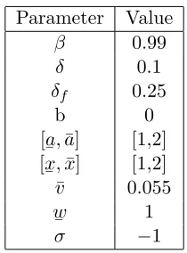
1.6 Comparative Statics and Numerical Results . . . 37
1.6.1 Matching Surface . . . 37
1.6.2 Comparative Statics . . . 38
1.6.2.1 Calibration . . . 39
1.6.2.2 Statics . . . 40
1.7 Empirics . . . 42
1.8 Conclusion . . . 47
2 Labor Reallocation and Sectoral Shocks 49 2.1 Introduction . . . 49
2.2 Data . . . 52
2.2.1 Sectoral Output . . . 53
2.2.2 IO Architecture . . . 54
2.2.3 Capital Flows . . . 55
2.2.4 Intersectoral Labor Movement . . . 56
2.2.4.1 The Cleaning Algorithm . . . 57
2.2.5 The Structure of Re-allocation . . . 59
2.3.1 Firms . . . 61
2.3.1.1 Final Goods . . . 61
2.3.1.2 Inputs . . . 62
2.3.1.3 Prices . . . 63
2.3.1.4 Decision Problem . . . 63
2.3.2 Workers . . . 64
2.3.2.1 Decision Problem . . . 65
2.3.2.2 Aggregate Worker Flows . . . 65
2.4 System Reduction and Approximation . . . 67
2.4.1 Blanchard Kahn and Approximation . . . 67
2.5 The Model Filter . . . 68
2.6 Factor Analysis . . . 69
2.7 Calibration . . . 70
2.8 Results . . . 72
2.9 Conclusion . . . 75
3 Product Search, Markups and Variety 79 3.1 Introduction . . . 79
3.2 The Model . . . 83
3.2.1 The Shopping Space . . . 83
3.2.2 Sellers . . . 84
3.2.3 The Firm’s Objective . . . 86
3.2.4 The Linear Case . . . 87
3.2.4.1 Competition vs. Concentration . . . 90
3.2.5 The Log Utility Case . . . 94
3.2.6 The Consumer’s Problem . . . 95
3.4 Conclusion . . . 101
List of Tables
1.1 Baseline Model Parameters . . . 40
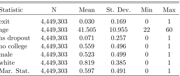
1.2 Individual Level Variables . . . 44
1.3 Market Level Variables . . . 45
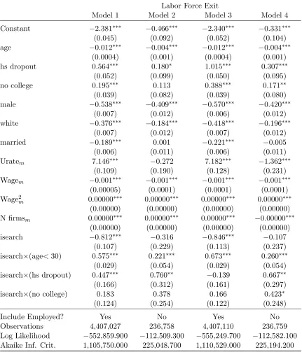
1.4 Logistic Regressions . . . 46
2.1 Summary Statistics for Sectoral Output . . . 53
List of Figures
1.1 Labor Force Participation . . . 2
1.2 Example Solution . . . 28
1.3 Matching Surfaces . . . 38
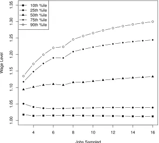
1.4 Wage Inequality . . . 41
1.5 Comparative Statics . . . 42
2.1 Distribution of Output Cross-Correlations . . . 54
2.2 Distribution of Normalized Outdegrees for Material Network . . . 55
2.3 Log Test Stat for Worker Reallocation . . . 60
3.1 Ecommerce . . . 80
3.2 Employees Per Firm . . . 82
3.3 Gamma Densities and Price Schedules . . . 89
3.4 Search Strategy . . . 98
Chapter 1
Wage Inequality and Labor Force
Participation in a
Simultaneous Random Search
Environment
1.1
Introduction
An increasing proportion of job search and hiring now occurs online. According to the survey
SilkRoad (2017), in 2017 over 50% of interviews are now sourced through online contacts.
In this same survey, the conversion rates of external application to interview and external
interview to hire are 33:1 and 3:1 respectively, combining to suggest that every vacancy
that is filled through online sources will require on average ∼ 99 applications. Similarly,
Marinescu and Wolthoff (2015) find using data from CareerBuilder.com that there were
59 applications per vacancy on that website. Compare this number to that reported in
Faberman and Menzio (2018) from the 1982 Employment Opportunity Pilot Project who
one week (and notably fewer applications for all other openings.)
Corresponding with the rise in online job search has been a marked decrease in labor
force participation. As seen in 1.1, from its peak above 67% in 2000, participation has fallen
to under 63% in 2018.
Figure 1.1: Labor Force Participation
Yet this transition in labor force participation has not occurred equally for all groups.
According to Frazis (2017), the two single biggest predictors of labor force exit over the
period 2005-2015 were education and age of the worker–with younger, less-educated workers
exiting the labor force in much higher quantities.
As I will suggest later in the paper, labor force exit by predominantly younger and
lower skilled workers can be explained by a permanent “crowding out” effect brought on by
a rise in search efficiency. In a low information environment–where firms come into contact
with few workers–the lowest skilled in any distribution have a chance of “getting lucky”,
and being the best candidate around for the job. In the alternative–when firms sample a
large amount of potential workers–it is extremely unlikely that this same worker will prove
to be the best candidate for any job. Hence, their motivation to search will dry up and they
will exit the labor market. In a sense, workers of low skill benefit from search frictions, in
This notion of “crowding out” is an old concept in the job search literature, though
usually cast in the context of movements over the business cycle. As labor conditions
worsen, firms can increase their hiring standards due to an increased pool of workers. To
my knowledge, this is the first paper that suggests this effect being generated by long-run
changes in search technology as opposed to productivity movements over the business cycle.
Concomitant with a fall in labor force participation has been an increase in wage
inequality. Pew Research (2018) documents that real wage increases since 2000 for the
lowest and highest decile of earners have been 3% and 15.7% respectively. The current
paper suggests a novel contributor to this rising wage inequality: as worker-firm contacts
increase–that is, as search frictions decline–competition for workers will increase and the
incentives to post high wages will increase disproportionately for already high-paying firms.
In the wage-posting environment I will build, posting a higher wage gives a notion of
preference to a firm in their worker choice process. When firms are more informed about the
existence of good workers they can choose more discriminately, and the value of this choice
preference increases along with the incentive to raise wages. The nature of this incentive
is predominately a competitive one–deviations yield preference at the cost of others–and
so higher-ranked firms will be disproportionately affected, as they face more competition
“from below” than lower-ranked firms. Higher-ranked firms will be induced to raise their
wages, and higher-ranked workers will more efficiently match with them.
The model used to demonstrate the twin effects of crowding out and wage inequality
will feature simultaneous random search. Workers will be allowed to sample firms
ran-domly at will; but, they will face a cost to do so. Time will be discrete, and the competition
amongst firms and workers in the matching space will be made explicit–firms will be
con-tacted by multiple workers and will choose the best candidate willing to work for them, given
that worker’s other contacts–i.e. a pairwise-stable matching. The pairwise stable matching
will occur in the context of (and be enabled by) wage posting with full commitment.
matching problem is tractable and it is governed by the solution of a system of two
first-order partial differential equations. In equilibrium, the solution of this system pins down
the expectations of workers and firms about their prospects of participating in the matching
market. I will approximate the solution to this system via pseudospectral element methods
with an endogenous division of the subdomain. In a technical sense, this paper will be of
interest to those who wish to solve such problems–a common occurrence when distributions
must be solved numerically within a model with actionable regions. The pseudospectral
methods must be implemented on subdivisions of the matching region because the model will
feature nondifferentiabilities and occasionally discontinuities–a fact that I will document.
After the model exposition, I will provide evidence of a link between labor force
participation and cheap search in the microdata of the Consumer Population Survey from
the BEA. Within an econometric specification, cheap search will be identified through the
Computer and Internet Use Supplement to the CPS survey, which asks users about internet
job search. A logistic regression specification will demonstrate a strong statistical link
between the presence of internet search and labor force exit by specifically younger and
uneducated workers—which represent two proxies for worker rank.
This paper joins a large and growing literature on matching environments with
ran-dom search frictions. Most of this literature focuses on sequential search (see: Shimer and
Smith (2000) for a pioneering example and Chade et al. (2017) for a thorough review.) I
have chosen to model simultaneous search here for a few reasons.
The first is that it more accurately captures the decision problem faced by firms.
Gen-erally firms receive a slew of applications, they sort through them and make offers in order
of their preferred candidates. This logic is more closely mimicked in a simultaneous search
environment and so allocations are likely to be better represented that way. Obversely, in a
sequential search model, a firm is merely looking for the first acceptable candidate to arrive,
up–especially as the rate of contacts increases to many per day–to the intuitive picture of
a firm sorting through applications.
The second is that search competition in a discrete time setting is more amendable to
calibration and estimation. Data are received in discrete form; and indeed, continuous time
models are discretized vis-a-vis time in order to be fit to the data. Simultaneous search
therefore provides a ready form to be fit to data, as well as to serve as a check on the
prescriptions of the numerous models discretized from continuous time.
Another major contrast between this paper and the broader literature is the use of
wage-posting. A majority of models of search and matching rely on a bargaining game to
solve the bilateral monopoly problem of a matched firm and worker. Bargaining serves to
lend a great deal of tractability to what are otherwise complicated models. The decision
to use wage posting in this paper was made for two reasons. First, wage-posting generally
characterizes the behavior of firms looking to hire for low-skilled positions in the US labor
market. Therefore, wage-posting is a more natural choice when modeling the behavior of
lower-ranked workers. Additionally, wage-posting serves as a way to clear the matching
market in a simultaneous search and matching setting.
Several related papers to the current one are as follows. Uren and Virag (2011) build a
wage posting model in a search environment in continuous time. Their goal is to demonstrate
how changes in the production function–notably via skill-biased technological change–can
induce rising wage inequality. The current paper focuses instead on how the changing search
technology can generate effects on labor force participation and wage inequality.
There is also an emerging literature on the increasing efficiency of search or,
equiv-alently, in falling search frictions. Martellini and Menzio (2018) find evidence that search
frictions have declined considerably in recent years, and provide a theoretical rationalization
of how stationarity of key labor statistics can be preserved in spite of falling search costs. In
another vein, Hursey (2018) shows that in a product search environment, increasing search
the shape of idiosyncratic tastes. The current paper will employ a similar mechanism to the
case in Hursey (2018) where idiosyncratic tastes are small in magnitude: the competitive
effects of search will dominate and force the lowest performers out of a market.
The remaining paper will be organized into seven sections. Section 2 will present
the model environment, followed by the pairwise stable matching algorithm in Section 3.
Section 4 will embed the matching space into a general equilibrium framework, while Section
5 will provide details on the computation of the model via pseudospectral methods. Section
6 will show numerical results and Section 7 will include empirical ones. Section 8 concludes.
1.2
Model Environment
The model is set in discrete time with infinite periods denoted by t ∈ {0,1, ...}. There
are two types of agents: workers, who are endowed with an indivisible unit of labor and
an idiosyncratic skill level a; and firms, to whom the workers’ labor can be sold and who
own their own technology characterized by the functiony :A×X → R which maps their
efficiency level x and the ability of their workera into an output quantityy.
The workers constitute a positive measure of agents, normalized to 1. Of those,eare
matched with the same number of firms at any given time while 1−eare unmatched. There
is a positive measure V of unmatched firms/vacancies which is composed of a measure of
different efficiency firms such thatRXv(t)dt=V. Therefore, the distribution of efficiencies
of actively searching firms can be given as F(x) =
Rx
¯
x v(t)dt
V .
The distribution of the abilities of workers in the population as a whole is described
by the CDF Ω :A→[0,1] which gives the probability Ω(a) that a randomly drawn worker
from the overall population will exhibit less ability thana. The efficiencies of firms are also
described by a CDF Λ :X → [0,1]. This CDF describes the distribution of efficiencies of
putative firms; that is, those firms who could potentially enter the matching market should
efficiencies is given by ¯v.
Each firm and worker can be of two types: matched; or unmatched. At the beginning
of the period production occurs and matched worker-firm pairs produce using their
tech-nology while unmatched workers engage in home production that yields a payoff b ∈ R+.
Matched workers are paid a contracted wagewthat is unchanged over the life of the match.
Unmatched firms produce nothing.
After production, unemployed workers can engage in costly search in order to match
with an unmatched firm and begin employment. There is no search on the job but it would
be an interesting direction for future research. Workers own a search technology z:R+ →
R+ that allows them to convert costly effort into an expected number of connections with
unmatched firms. The mechanism by which connections are converted into consummated
matches will be described later in the section on the matching algorithm.
The unmatched firms over which the unemployed will search are operating a vacancy
with which they have been endowed. At the end of the period, unmatched firms’ vacancies
have a probabilityδf of exploding, while a consummated match has a probabilityδof doing
so. As separation occurs after search, separated workers do not engage in it in the period
they lose their job.
1.2.1 The Search Process
As stated in the previous section, workers can exert effort to match with z number of
expected vacancies. This subsection will describe the manner in which those connections
are apportioned amongst firms. This process will take the form of growing a bipartite graph
between the measures of firms and workers within the model.
The very first action in the search phase of the model is wage posting. Firms post
a wage w∈R to which they are committed during the period–meaning it is unchangeable
throughout the process of search and matching and must be paid over the life of any
both endogenous and of common knowledge. Upon meeting a firm, an unemployed worker
observes its posted wage.
Let zt(a) represent the expected number of connections obtained by the worker of
ability a. The actual number of connections of this worker is a random variable described
by the discrete distribution
Θ0(a) :Z×R+ →[0,1]
. For the remainder of this paper I will assume than this distribution is a Poisson distribution
parameterized by rate zt(a). A Poisson distribution will deliver more tractable quantities
for the matching process; though other distributions may be used.
Let the measure of unemployed workers of ability aat the beginning of a period be
given byut(a). Then the total measure of connections generated by the unemployed at the
beginning of the period is given by the quantity:
Z ≡
Z
s∈A
z(s)u0(s)ds
. These connections need to be distributed over the total measure of vacancies V.
The allocation of connections is at its core an example of generating a bipartite graph
between a positive measureUtof unemployed andVtof vacancies. Let Σ = (U, V, ε) describe
this graph withU,V the vertices andεrepresenting the set of edges between them. For this
graph to be consistent, a rule for distributing connections overU×V needs to be proposed
such that the total number of connections equalsZtand the number of connections possessed
by both sides of the graph clear:
Zt=Vt
Z
s∈W
r(s)dF(s)
eration of the graph is the following one. It features independent allocation over vacancies
and workers, i.e. the probability that a connection belonging to a worker of ability a also
belongs to a firm of wage w does not depend on aor w. Further, firms receive a random
allocation of connections within wage levels that is itself described by a Poisson distribution.
That is, all firms receive a random allocation of connections given by a draw from Poisson
distribution with rater(w) =r ∀w. To sum up, the edge clearing of the bipartite graph
is described by the equation:
Zt≡
Z
s∈A
z(s)u0(s)ds=Vt
Z
s∈W
r(s)dF(s) =rVt
The method of graph generation given above which gives no preferential attachment
based on agent type is in some sense the most random–or undirected–possible. The wages
and abilities of workers give no guidance to which connection are formed between which
agents. While this assumption might not be entirely realistic, I consider it the ideal starting
point for an analysis of random, simultaneous search. Modifications which give preferential
attachment based on wage or ability–rendering search somewhat directed–is both beyond
the scope of this paper and a very interesting direction for future research.
1.3
The Matching Algorithm
The purpose of this section is to describe the algorithm used to generate a pairwise stable
matching between unemployed workers and vacancies. First, a concept of firm ordering
based on posted wage will be introduced. The algorithm is then cast in terms of movement
along the queue generated by such an ordering. The initial system over the countably infinite
equations of the graph degree distribution will be reduced into a system of two partial
1.3.1 Firm Ordering
In order to execute the algorithm, a concept of firm ordering needs to be established. The
ordering describes the preference given to firms in their decision-making process, meaning
a higher-order firm’s decision will always take precedent over a lower. Simply, the ordering
of firms is determined by their wage.
Let F(w) represent the CDF of wages posted by firms in equilibrium and let w(F)
represent its inverse. IfF(w) is continuous at a pointw, a measure 0 set of firms is choosing
and therefore a firm with wagew faces a zero probability of a rival claim to a given worker.
However, if a mass point exists inF(w) and two or more firms covet the same worker, it is
assumed the worker chooses randomly between them. However, this cannot occur according
to the following,
Proposition 1.3.1. F(w) contains no mass points
Proof. SupposeF contains a mass point atwand consider a firm with a preferred candidate.
Because there is a positive measure of firms choosing along with this firm, they face a
non-zero probability p of losing this preferred candidate through randomization; while, a wage
w+εwould have guaranteed recruitment for anyε >0. Taking expectations implies there
is a discontinuous gain and∃ε that is a profitable deviation.
The matching algorithm, in order to generate a pairwise-stable matching, can be
understood to progress sequentially along the ordering generated by wages. Starting at
F = 1 and progressing downward in the rankings to 0, all firms posting a wage of w(F)
make their selection of their preferred candidate from amongst their available connections
(if any).
The firm ranking F as a state variable in the algorithm can therefore be thought
of, in one interpretation, as similar to time in a differential equation–where each period is
interpretation of the device used to generate the calculation of the pairwise stable matching
and need not be taken explicitly.
1.3.2 Preliminaries to the Algorithm
Before describing the algorithm, several objects need to be posited which will be identified
as equilibrium objects by the firm and worker problems later in the paper.
The first of these is
¯a(F), which gives the lowest overall quality worker that a firm at
queue rank F would consider hiring; that is, it is its reservation quality. Obversely,
¯
F(a)
gives the lowest-ranked firm a worker of ability level a would be willing to accept. This
immediately implies thatw(
¯
F(a)) is workera’s reservation wage.
If the production function y(a, x) is increasing in a, then
¯
F(a) is increasing and
therefore can be inverted for ¯a(F), the highest ability worker willing to accept an offer from
firm rank F (and wage w(F)). It will be convention for the algorithm that those workers
whose reservation wage has passed will exit the matching market and their links will be
destroyed.
Lastly, letu(a, F) represent the remaining measure of unemployed workers of ability
levelaafter all firms with efficiency greater thanF have moved. And let the total number of
links possessed by workers (and firms through market clearing) at a pointF in the algorithm
be given by the function
˜
z(F) = Z ¯a(F)
¯
a
z(s)u(s, F)ds
1.3.3 The Algorithm
Given the policy rules ¯
F and ¯
athis subsection will describe the allocation that occurs from
the pairwise stable matching algorithm. It will first describe the firm’s side of the algorithm.
Firms will possess at any given queue position a certain number of potential connections
with workers. As firms above a given firm move, these connections will disappear as either
After describing the degree distribution of active connections, I will detail the firm’s
problem. This will provide conditions under which the wage posted by a firm is increasing
in its efficiency–meaning more efficient firms post higher wages. Therefore, efficiency, wage,
and queue order are all monotonically related, and efficiency may serve as a sufficient
statistic for queue order. The firm’s side of the algorithm will deliver the equilibrium
distribution over thebest candidate that a firm can expect to hire from their basket.
The workers’ side of the algorithm will be described after the firms’. Workers similarly
will have a degree distribution, or distribution over active connections to firms. They will
be hired by a given firm if their overall quality is the highest in that firm’s basket, and
that quality is above the firm’s reservation quality. The result of the worker’s side of the
matching algorithm will be a partial differential equation that describes the instantaneous
probability of a worker of abilityaof being hired at the queue position of firm efficiencyx.
This will combine with the condition on firm’s expectations to fully describe the dynamics
of the matching algorithm.
1.3.3.1 The Firm Side
Let φ(t, F) = {φi(t, F)} describe the probability mass of number of active connections
of a firm of type t after all ˆF ∈ [F,1] firms have made their selections, also known as
the conditional degree distribution. So for example, the initial distribution is given by
φi(t,1) =e−r r
i
i!, or the Poisson pmf.
The following proposition shows that φ() will be identical for all firms remaining in
the algorithm by showing the three conditions that pin down its dynamics are identical for
those firms.
Proposition 1.3.2. φ(t, F) =φ(F) ∀t≤F
Proof. Lett1, t2 < F be two ranks lower than the currently choosing one. φ(t1,1) =φ(t2,1)
of their type by assumption. Lastly, firm selection of candidates does not condition on
candidate’s connections to other firms ⇒
∂φ
∂F(t1, F) = ∂φ ∂F(t2, F)
As a result, separate distributions need not be considered for each firm rank. Therefore
let q(F) represent the common, instantaneous rate of link destruction for firms who have
not moved yet, meaning the unconditional rate at which a firm’s connections disappear as
higher-ranked firms move. The sources of link destruction are twofold: the rate at which
workers are stolen by firms of a higher wage, and the number of workers who exit the market
because their reservation rank ¯
F has passed.
The evolution of the distributionφcan be described via the differential equation
˙
φj(F) = [jφj(F)−(j+ 1)φj+1(F)]q(F)
For an infinitesimal change in the queue, each bin in the degree distribution sees an
inflow from the bin above it equal to (j+ 1)φj+1(w)q(w) which is the rate at which the
remaining firms lose their j+ 1 links times the measure in that bin. Similarly, the bin at
j loses its own denizens at an analogous rate times its own measure. Putting these two
together yields the differential equation above.
These differential equations over all j create a countably infinite system of linear
in matrix notation as
˙
φ(F)0=φ(F)0
−q(F) 0 0 0
2q(F) −2q(F) 0 0
0 3q(F) −3q(F) 0
0 0 ... ...
which is a state-dependent, continuous-time, infinite, non-homogeneous Markov chain where
the states are the bins in the degree distribution given by the vectorφ(F).
Proposition 1.3.3. Let q˜(F) = RF1q(t)dt. When the initial degree distribution is Poisson
with rate r, the firms’ degree distribution for the matching algorithm is given by
φj(F) =
(re−q˜(F))j
j! e
−re−q˜(F)
Proof. By direct inspection
If a more constructive proof is desired, one can use the matrix exponential form from
the Markov Process. Note that the degree distribution of links over firms remains Poisson
throughout the algorithm, with the rate parameter now given by re−q˜(F), that is, initial
rate degraded by outflows.
For now, assume that there exists a distribution over ability level for all of the extant
links in the algorithm at any given position F in the algorithm. That is, there exists a
function ˜H(a, F) with support [
¯
a,¯a] which gives the probability that a randomly selected
connection between a worker and a firm will have a quality less than or equal toaafter all
firms aboveF have made their decision.
Consider a firm that has i active links and is making its decision about whom to
hire from its available pool of iworkers. The distribution describing the talent level of the
Therefore, putting this together with the derived degree distribution for firms, theexpected
pseudo distribution from which a firm will hire its worker at queue positionF conditional
on having at least one connection and choosing the best available worker is given by
H(a, F) =X
i
φi(F) ˜H(a, F)i
=e−re−q˜(F)X
i
(re−q˜(F)H˜(a, F))i
i!
=e−r(1−H˜(a,F))e−q˜(F)
The program of a firm with efficiency levelxcan now be given. A matched firm with
efficiencyx, qualityq and wagew produces the following lifetime value function:
Jm(x, q, w) =
y(x, q)−w
1−β(1−δ)
Therefore, the program of an unmatched firm with efficiencyx is given by:
J(x) = max
q,F β
Z ∞
q
y(x, s)−w(F)
1−β(1−δ) dH(s, F) +H(q, x)(1−δf)Jt+1(x)
The firm has two choices to make. The first involves the lowest quality match it would
accept. The second is the position in the queue that the firm would like to occupy. The
cost for slotting at the queue position F is that the firm must post the wage w(F), or the
quantile ofF, that guarantees it is theFth ranked firm in the wage distribution.
In order to make x a sufficient statistic, it is required that the decision rule F(x) is
increasing; that is, the queue position chosen by a firm is an increasing function of their
efficiency level. The following proof establishes this as the case for a production function of
the formy(x, a) =xαa1−α. Any CES production function with a lower elasticity will then
obtain as well.
Proof. Suppose there are x < x0 s.t. F(x) =F > F(x0) =F0.
⇒J(x0, F)> J(x0, F) andJ(x, F)> J(x, F0)
⇐⇒ J(x0, F)−J(x, F)< J(x0, F0)−J(x, F0)
⇐⇒ R∞
¯q
(x0−x)sdH(s, F)<R∞
¯q
0 (x0−x)sdH(s, F)
⇐⇒ R∞
¯q
sdH(s, F)<R∞ ¯q
0 sdH(s, F)
⇐⇒ J(x, F0)> J(x, F) ⇒⇐
.
Given a function that ensures a monotonic queue decision rule, the firm’s efficiency
can then serve as the sufficient statistic for the state of both the wage distribution and the
queue order as the algorithm progresses. Thus, takew(x) =w(F(x)) to be the wage posted
by firm x, F(x) to be the queue position of firm x, and H(a, x) = H(a, F(x)) to be the
quality pseudo-distribution that firm x guarantees itself by obtaining queue positionF.
The firm’s side of the algorithm delivers the distributionH(a, x) that is faced by the
average firm of a given efficiency x. The next section will use this equilibrium object to
determine how workers outflow from the market. It will first demonstrate that the object
H(a, x) is an exponential of the total mass of links with quality above the worker’s abilitya.
Then, it will use this fact to deliver a two-equation system of partial differential equations
that determine the instantaneous probability of being hired throughout the algorithm.
1.3.3.2 Workers
Workers who are still in the market maintain a set of active links from which they could
potentially be hired. On the other end of any of these links is a firm also connected to other
workers.
Consider a given position in the queue,x. At that position, an instantaneous
propor-tion of Ff((xx)) links are being actively considered by firms. Now consider a worker of ability
preferred candidate is
P
i≥1φi(x)iH˜(a, x)i−1
P
i≥1φi(x)
=e−r(1−H˜(aξ,x)e−q˜(x) =H(a, x)
The worker considers the distribution over how many other links the firms might be
connected to, and the probability that any of those other connections is owned by a worker
of higher ability. Perhaps unsurprisingly, this hiring probability is exactly the first order
pseudo-distribution that firms expect when entering the market.
Let p(a, x) represent the instantaneous probability of any of a worker’s links being
converted into a job offer, this probability is given as
p(a, x) =
f(x)H(a,x)
x a≥¯a(x)
0 o.w.
with the complementary rate that a link does not yield a hire and is destroyed given by:
γ(a, F) =
1−f(x)Hx(a,x) a <
¯a(x)
1 o.w.
Then the following differential equations represent the measure of unemployed workers
of ability level awithj active connections to firms remaining in the algorithm:
˙
mj(a, x) =jmj(a, x)(p(a, x) +γ(a, x))−(j+ 1)mj+1(a, x)γ(a, x)
mj(a,x¯) =ut(a)e−z(a)
z(a)j
j!
workers see outflow from havingj connections equal to the sum of the rates of link
destruction and hiring, and at rate γ(a, x) they have a link destroyed and flow into the j
Proposition 1.3.5. mi(a, x) is given as
mi(a, x) =ut(a)
(z(a)F(x))i
i! e
−z(a)
h
F(x)+R¯x(a)
x f(t)H(a,t)dt
i
Proof. By direct inspection
summing up the measure of workers over all bins yields the desired measure of workers
remaining of abilityaat a pointx in the algorithm:
Proposition 1.3.6. u(a, x) is given by
u(a, x) =ut(a)e−
z(a)
v
Rx¯(a)
x v(t)H(a,t)dt
The remaining measure of unemployed of ability a outflow at a rate given by the
expected number of links they received, times the product of their rank in the first order
distributionH(a, x) with the probability mass of vacancies atx.
As stated previously, at any point in the algorithm, the number of links possessed by
firms and workers must add up, this can now be precisely given by the following condition:
vF(x)X
i
φi(x)i=
Z ¯a(x)
¯
a
X
j
mj(s, x)ds
⇒vre−q˜(x)= Z ¯a(x)
¯
a
z(s)u(s, x)ds
Returning now to the first order distribution in order to close the algorithm. Recall
that ˜H(a, x) was the distribution of ability over links from whence the first order distribution
was derived. This can now be defined as
˜
H(a, x) = Ra
¯a
z(s)u(s, x)ds
R¯a(x) ¯
which, when plugged into the earlier derived expression for the first order distribution gives
H(a, x) =e−r(1−H˜(a,x))e−q˜(x)
=e−v1
R¯a(x)
a z(s)u(s,x)ds
The pseudo probability that the ability of the best expected candidate of a firm is less than
or equal to a is a negative exponential of the ratio of the mass of links of greater ability
thanato the mass of firms remaining in the market.
Note that the term in the exponential has a similar flavor to the vacancy
unemploy-ment ratio from search and matching models, and in some sense captures the ”tightness”
of the market, modified to include the number of links that workers possess. In fact, were
search behavior to be identical for all workers, such thatz(a) =z, the term would be exactly
F(x)z
R¯a(x)
a u(s, x)ds
F(x)v =F(x)z U(x)
V(x)
The two objects thus identified, H(a,x) and u(a,x), sufficiently describe the execution
of the matching algorithm and the expectations of workers and firms respectively about
their prospects in the search-and-matching market. Differentiating these two objects with
respect toaand x respectively yields the following system of partial differential equations
Ha(a, x) =
z(a)
v H(a, x)u(a, x)
ux(a, x) =
z(a)v(x)
v H(a, x)u(a, x)
(1.1)
with boundary condition for H given by H(¯a(x), x) = 1 and the boundary condition for u
to be given later in the equilibrium section.
Proposition 1.3.7. The matching algorithm is pairwise stable
Proof. Assume a putative, preferred bilateral deviation byx,a. xcould have chosenawith
1.4
Existence, Uniqueness and Topology of Equilibrium
The matching algorithm describes the microstructure of the matching market, and this
section will incorporate that microstructure into a dynamic, general equilibrium framework.
The equilibrium will exhibit a block structure, and its existence and uniqueness will be
established in a manner corresponding to that block structure.
1.4.1 Workers
Workers can be either employed or unemployed. If employed, a worker is paid their
con-tracted wage until the match is separated and they rejoin the pool of unemployed, implying
a value function for a contracted worker of
Vt(a, w) =w+βE[(1−δ)Vt+1(a, w) +δUt+1(a)]
An unemployed worker engages in home production in the beginning of a period.
They can then engage in costly search, hoping to secure a job for the following period but
must pay a cost given byξ(z) in order to search with intensity z. As seen in the matching
algorithm section, the mass of workers that remains after all firms above x have moved is
given by u(a, x), then n(a, x) =u(a, x)/ut(a) is the probability that a worker of abilitya
remains unemployed. The worker’s problem can then be stated as
Ut(a) =b−ξ(z) + max
z,x βE
" Z x¯(a)
x
Vt+1(a, w(t))d[n(a, t)] +n(a, F(x))Ut+1(a) #
The optimal policy for a reservation level for a worker is given by
¯
which implies a worker will accept a wage up until they are indifferent between accepting
that wage and returning to unemployment.
Forz(a), the policy rule is given implicitly by
−z(a)β
Z x¯(a)
¯x(a)
Vt+1(a, w(t))d[n(a, t) lnn(a, t)] =ξ0(z(a))
. Here the worker trades off the cost of engaging in extra search relative to the improvement
in their employment prospects, given the behavior of all other agents.
In any steady state equilibrium,Vt=V, Ut=U ∀t, and these reduce to
V(a, w) = 1 ˜
β [w+βδU(a)]
⇒U(a) = 1 ˜
β[1/β+δ−n(a,¯x(a))]
−1
" ˜
β
βb−ξ(z) +
Z F¯(a)
F(R)
w(t)d[n(a, t)] #
while the policy rules are
¯
x:
¯x(a) = inf{x:w(x)≥(1−β)U(a)}
z: −z(a)β
Z x¯(a)
¯
x(a)
w(t)d[n(a, t) lnn(a, t)] = β˜
βξ
0(z(a))
1.4.2 Firms
The program of a firm can now be restated from the matching algorithm section in terms
of efficiencies. A firm of type x solves the objective function given by:
J(x) = max
a,˜x β
" Z ¯a(x)
a
y(x, s)−w(˜x)
1−β(1−δ) dH(s,x˜) +H(a,x˜)(1−δf)Jt+1(x)
#
. A firm chooses their reservation abilityaand which type they would like to try to mimic
case that ˜x=x. Where the wage distribution is differentiable, the condition governing the
optimal wage policy of firms–after steady state conditions have been imposed and a healthy
serving of algebra–is given by:
w0(x) =−
R¯a(x) ¯a(x)
ya(x, s)Hx(s, x)ds
1−H(
¯
a(x), x) (1.2)
Hxis the derivative ofHwith respect to firm typex(and queue position modulo a constant),
and is therefore an expression of how the distribution of best-available workers improves as
one moves up the queue. Ergo, it captures in the wage-equilibrium condition the benefits
of posting a higher wage in terms of the improvement of the talent pool a firm can recruit
from. DifferentiatingH(a, x) yieldsHx as:
Hx(a, x) =−
"
z(¯a(x))
v u(¯a(x), x)¯a
0(x)− 1
v
Z ¯a(x)
a
z(s)ux(s, x)ds
#
H(a, x)
There are two sources of improvement in the talent pool present in this derivative. The
first term in brackets represents the improvement in the upper bound of the support of the
distribution. When firms increase their wages, they increase the best quality worker that
would be willing to accept them as an employer. Call this effect theacceptance effect.
The second term in brackets represents the marginal improvement in the quality of
remaining workers in the pool when moving up the queue–workers of typeaare flowing out
of the market at rateux(a, x). Call this effect thecompetition effect.
The firm, then, chooses their queue position to optimally trade off the benefit of
moving up the queue–given by the expectation of the improvement in the marginal product
of workers recruitable by the firm from both the acceptance and competition effect–against
the costs of doing so, represented simply by the wage.
To complete the firm’s wage policy, a boundary condition needs to be imposed on the
imposed ¯
w, or a condition requiring that the lowest paying firm has no incentive to deviate
downward in wage. I will assume for now a binding minimum wage policy ¯
w posted by the
lowest ranked firm.
The reservation policy of the firm is straightforward, given by
y(x,¯a(x))−w(x) = ˜β(1−δf)J(x)
. The firm is willing to accept a worker up until the point where the gains from waiting
and searching again are larger than employing that worker.
1.4.3 Equilibrium
The last element of the model that needs to be pinned down prior to defining equilibrium
is the transition of states between periods.
The remaining mass of unemployed workers of typea after the matching market is
concluded is given byu(a,
¯
x(a)), while (u(a,x¯(a))−u(a,
¯
x(a)) have transitioned to
employ-ment. Obversely, (ω(a)−u(a,x¯(a)) is the mass of abilityathat starts a period employed,δ
of which lose their job and enter the unemployment pool for the next period. (Recall that
ω describes the distribution over talent in the unit population of workers) Therefore, the
steady state condition governing worker flows is given by
uss(a) =u(a,x¯) =
δω(a) +u(a,
¯
x)
1 +δ
For firms, an inflow of ¯v new vacancies enter the matching market in any period,
distributed over efficiencies by the functionλ(x). 1−H(
¯a(x), x) of these firms fail to find a
match, of which δf are destroyed. Therefore the steady state of the law of motion for firm
measures is given by
v(x) = vλ¯ (x)
1−H(
¯
.
An Equilibrium for the model can now be defined.
Definition 1.4.1. A stationary equilibrium of the model is defined as: Value functions
J, U, V; policy functions
¯
x(a), z(a) for the workers and w(x),
¯
a(x) for the firms; measures
H(a, x), u(a, x), v(x) governing the populations of agents such that
1. w(x),
¯
a(x) solves the firm’s problem given distributions and policy rules
2.
¯
x(a), z(a) solve the worker’s problem given distributions and policy rules
3. H(a, x), u(a, x) solve (1.1), given
¯a(x), ¯x(a), z(a), with boundary conditions
consis-tent with functions uss(a), v(x)
1.4.4 Existence, Uniqueness and Topology
The structure of the equilibrium will exhibit a block-like nature–with discontinuities or
non-differentiabilites being propagated downward throughout the matching market.
To begin, a condition describing the local differential equation of worker reservation
policy to match that of the firm needs to be derived. Differentiating the worker’s policy
function gives
(1
β +δ−n(a,¯x))w
0
( ¯
x(a)) ¯
x0(a) =−
Z x¯(a)
¯x(a)
w0(t)na(a, t)dt
The worker’s reservation rule ¯
x(a) reflects the relationship between the improving prospects
of a worker as ability increases and the change in their reservation wage.
na(a, t) represents how a worker’s prospects improve in the matching market as their
ability improves. Differentiating n(a, x) gives
na(a, x) =
"
−z(a)v(¯x(a))
v H(a,x¯(a))¯x 0
(a)−z(a)
v
Z x¯(a)
x
v(t)Ha(a, t)dt
#
. Similar to the firm’s rule, there are two effects present. The first term in brackets gives
the acceptance effect for the worker. As ability improves, the highest efficiency firm that
would be willing to hire the worker improves by ¯x0(a), while a worker’s chance of being
the best candidate for that firm isH(a,x¯(a)). The second term represents the competition
effect for the worker, as their ability improves they marginally improve their prospects over
Ha(a, t) measure of candidates. Note the above does not contain the marginal effect from
on z(a) as this cancels with the cost of that search in the worker’s problem.
The above differential equation, when paired with the firm’s similar reservation
equa-tion, will describe a system of ordinary differential equations for the acceptance regions of
the agents in the model. However, as will be shown in the following section, the
accep-tance effects–being composed of the reservation rules of agents “above” the current state
in the matching algorithm–will introduce non-differential points. Therefore the equilibrium
existence will have to be proven piece-wise, which is done in the following section.
1.4.4.1 Existence and Topology
Define finite subdivisions of the firm efficiency support and worker ability support in the
following way. Initialize via
xNx = ¯x
aNa = ¯a
and
xNx−1 =¯x(¯a)
. Then define the subdivision iteratively via:
xi = max{
¯
x(
¯a(xi+2)),¯x}
ai= max{
¯
a( ¯
x(ai+2)), ¯
a}
Consider the highest ability worker ¯a. This worker will choose a reservation firm
¯
x(¯a) < x¯. Now consider the interval INx−1 = [xNx−1, xNx]. Within this interval, firms
can feasibly hire from any of the available population given a connection, as ¯a = ¯a(x).
Presupposing a boundary condition at ¯
wNx =
¯
x(¯a), the following proposition holds
Proposition 1.4.2. Given
¯
wNx a unique solution to the wage equation exists on INx.
Proof. By the Picard-Lindel¨of Theorem
Next, consider a second interval in the efficiency support of firms given byINx−2 =
[xNx−2, xNx−1]. As stated earlier, the policy function
¯
x(a) is increasing, therefore ¯a(x) is
increasing in equilibrium. Employ a change of variables to invert the condition describing
worker reservation values as
¯
a0(x) = (1/β+δ−n(¯a(x), x))w
0(x)
−R¯x(¯a(x))
x w
0(t)n
a(¯a(x), t)dt
(1.3)
Let xNx−2 be given by max{¯x,{x : ¯a(x) = aNa−1}}, and suppose a boundary condition
given by ¯wNx−2, then the following proposition holds:
Proposition 1.4.3. Given w¯Nx−2 and w on subdomainINx−1 a unique solution (w(x),¯a)
exists that solves the ODE system given by 1.2 and 1.3
Proof. By the Picard-Lindel¨of Theorem
.
It remains to be shown that the solution to the ODE system is in fact increasing in both
variables, as was assumed at the outset. The following proposition details the necessary
and sufficient condition for the equilibrium wage function to be continuous atx∗
Proposition 1.4.4. The equilibrium policies are continuous at xNx−1 =x
∗ ⇐⇒
Z x¯
x∗
w0(t)(n(¯a, t)(1−n(¯a, t))dt >(1/β+δ−n(¯a, x∗))n(¯a, x∗) R¯a(x∗)
¯a(x
∗) ya(s, x)H(s, x)ds
1−H(
¯
a(x∗), x∗)
Proof: See appendix.
To see when this will obtain, rewrite the coupled ODE system as
J(¯a, w)
w0
¯
a0
=G(¯a, w)
then, w0 and ¯a0 are positive iff the above proposition holds, which is merely a condition on
the determinant ofJ(¯a, w).
The intuition for the proof is the following. Atx∗, the acceptance effect begins to be in
effect for firms–the best candidate they can hire begins to degrade. This gives an increased
incentive, in equilibrium, for wages to fall as the queue progresses. However falling wages
feed back into the acceptance effect, such thatw0, ¯a0 are determined by the ODE system.
If the feedback effects are too strong, it can be impossible for an infinitesimal change in both
wages and ¯a0 to be consistent with equilibrium, so that a discontinuity in wmust occur.
What a discontinuity inw(x) implies is that the wage pdf,f(w) has a gap in it where
w(x) is discontinuous. The implication is that at these points, workers are sorted into
classes–or tiers–with stark differences in wages between them. We will see in the
computa-tional section that these equilibria are actually quite common for reasonable calibrations of
the model, and that sorting into tiers is generally the norm. That this granularity emerges
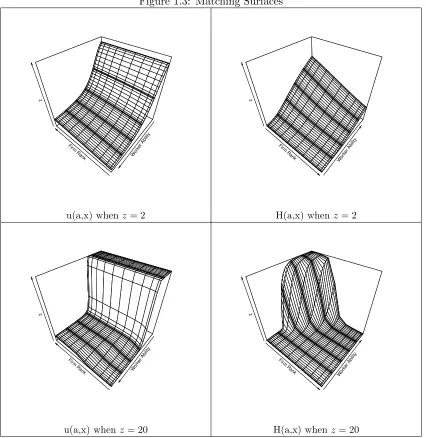
Figure 1.2: Example Solution
1.0 1.2 1.4 1.6 1.8 2.0
1.0
1.2
1.4
1.6
1.8
2.0
Firm Efficiency
W
or
k
er Ability
Acceptance Regions
Fir m Rank
Wor ker Ability z
u(a,x) on Acceptance Domain
1.5
Computation
This section describes the computational methods used to find an approximate solution to
the equilibrium conditions. As noted in the section on the topology of the equilibrium, the
{ai} and{xj} points represent non-differentiable points in the model. This fact, combined
with the need to impose boundary conditions in a dynamic general equilibrium framework,
necessitate a global solution method that can account for multiple subdomains.
Pseudospec-tral element methods are an ideal choice because of their amendability so such problems,
and because of their ease of numerical integration.
To give a sense of what kind of computational problem the equilibrium approximation
represents, Figure 1.2 plots an example acceptance region and surface plot for the u(a, x)
function. The grey lines in the acceptance domain represent the non-differentiable loci
that in a sense carve up the domain endogenously. These lines, along with the boundaries
represented by the acceptance functions ¯
x and ¯
a, will represent the boundaries of the mesh
1.5.1 Pseudospectral Element Methods
The structure of the equilibrium–in which multiple kinks and discontinuities will be
re-flected down the algorithm–requires a flexible computational approach to approximate.
This section will detail such an approach. It relies on pseudospectral element methods to
approximate both the policy functions and the surfaces of the distribution functions. The
subdomains will be determined endogenously according to the mapping of nondifferentiable
points down the matching queue. Thus, this section might be of interest to those looking
to approximate diffeo-algebraic equations on a flexible grid.
Pseudospectral methods involve approximating a function by assuming a projection
onto a functional basis. In this paper, I will be employing the basis of Chebyshev
poly-nomials. I will give a brief overview of the details of this method, but refer the interested
reader to Judd (1998) for a cursory introduction for economists, or Kopriva (2009) for a
more thorough coverage of the methods used here.
Chebyshev approximation involves approximating a function via
f(x) =X
i
ciψi(x)
where ψi are the Chebyshev polynomials of the first kind andci are the weights on those
polynomials. Chebyshev polynomials have nice properties of orthogonality, meaning, among
other things, that they provide a good approximating basis.
For the decision rules, the model requires approximatingNa−1 policy rules for the
workers, on the intervals defined by the partitioning algorithm that gives {ai}. Similarly,
the firm’s decision rules will be demarcated along a grid defined by the Nx −1 intervals
suggests the following approximation scheme for the decision rules:
¯
x(a) =γ(q(a)) =X
i
cgiψi(q(a))
q(a) = a−ai
ai+1−ai
where thecgi determine the weights andq(a) maps to the unit interval. z(a) can be defined
similarly.
Firms’ rules are approximated in a similar way on a given interval, with
w(x) =υ(r(x)) =X
i
cwiψi(r(x))
r(x) = x−xi
xi+1−xi
The surface distributions are also approximated with chebyshev polynomials. This is
accomplished via tensors of the single dimension polynomials, e.g.
f(x, y) =X
i
X
j
cijψi(x)ψj(y)
.
The mapping of the surfaces to squares, however, is slightly more complicated than
with the decision rules, because the domain on which they are defined is sometimes bounded
by the rules themselves–leading to endogenously-defined non-square surfaces. In order to
map the subdomains for these functions to the square, two types of mappings and their
relevant jacobians will be used. A vertical stretch mapping will map the bottom and top
boundaries–defined by curves–to the bottom and top of the square; while the horizontal
stretch will do the same for the right and left boundaries. In the case where the bounded
subdomain is three-sided, either mapping can be used, with a mapping between the corner
appeared to have little effect.
First define the mapping to a square for a rectangular surface defined by [ai, ai+1]×
[xj, xj+1] via
q(a, x) = a−ai
ai+1−ai
r(a, x) = x−xj
xj+1−xj
Now, suppose a surface is bounded by the rules ¯
a(x) along its lower boundary and
¯
a(x) withx∈[xj, xj+1] along its top boundary. Define the vertical stretch mapping as
q(a, x) = a−¯a(x) ¯
a(x)−
¯a(x)
r(a, x) = x−xj
xj+1−xj
. This will map the subdomain on which the surface is defined onto the square by stretching
it vertically according to the decision rules that bound it.
Alternatively, invert the bounding functions for
¯x(a) and ¯x(a) with a ∈ [ai, ai+1].
Define the horizontal stretch mapping as
q(a, x) = a−ai
ai+1−ai
r(a, x) = x−¯x(a) ¯
x(a)−
¯
x(a)
. This will map the subdomain on which the surface is defined onto the square by instead
stretching it horizontally. All three of these mappings will be used to approximate the
surfaces depending on how it is bounded and which decision rules are being updated and
therefore how the surfaces need be numerically integrated.
Given an appropriate mapping to the square, the surface functions can then be
ap-proximated as as
H(a, x) =B(q(a, x), r(a, x)) =X
i
X
j
cbijψi(q)ψj(r)
u(a, x) =D(q(a, x), r(a, x)) =X
i
X
j
cdijψi(q)ψj(r)
Obtaining approximations is then a matter of defining an appropriate concept of a
residual and minimizing that residual according to a chosen method. In this paper I will
minimize the residual at collocation points given by the Gauss-Chebyshev points of the
interval or surface in question.
The residuals for the surface functions are given by the PDE system that resulted
from the matching algorithm, given the decision rules of the firms and workers. For the
vertical stretch mapping, these are given by
GD ≡Dr(q, r)
1
∆x
−Dq(q, r)
q∆a
γ0(q(¯a(x)))(¯a(x)−
¯
a(x))+
(1−q)α0(r)
δx(¯a(x)−
¯
a(x)
− z(a(c, r))v(r)
v D(q, r)B(q, r)
GB≡Bc(q, r)
1 ¯
a(x)−
¯a(x)
−z(a(c, r))v(r)
v D(q, r)B(q, r)
where subscripts denote derivatives wrt that variable. These residuals come from the
re-quired change of variables to map the surface PDE to the square. The horizontal stretch
mappings are given similarly as
GD ≡Dr−
z(a(c, r))v(r)
v DB(¯x(a)−¯x(a))
GB ≡Bc
1
∆a
−Br
r∆x
α0(r(¯x(a)))(¯x(a)−
¯
x(a)) +
(1−r)γ0(c)
∆a(¯x(a)−
¯
x(a))
−z(a(c, r))v(r)
v DB
.
1.5.1.1 Collocation
Approximation will be obtained by miniziming the equilibrium residuals at collocation
points given by Nc+1 Gauss-Chebyshev points. These points are defined as
xj = cos
(j−1/2)π
where Nc is chosen to provide an adequate level of accuracy and represents the order of
the highest level of Chebyshev polynomial used. The Gauss-Chebyshev points represent
the roots of this highest order polynomial, and minimizing at these points yields a
nonlin-ear system of Nc+1 residual equations and Nc+1 unknown weights {ci} for the univariate
functions, and N2
c+1 residual equations and Nc2+1 unknown weights{cij} for the bivariate
surface equations.
While methods exist to collocate on sparser grids, e.g. Judd et al. (2014), there
are two reasons not to do so here. First is that numerical integration for the decision
rules will occur along the lines defined by the tensor product of the subdomain, so the
highest possible accuracy is ensured when the full tensor product is used. Second, as we
will see, the factorizations of the matrices representing the chebyshev polynomials at the
Gauss-Chebyshev points can be precomputed when the full tensor product is used–greatly
increasing the speed of computation by removing the need to invert large matrices.
The matrix of 2Nc2+1 residual equations for the distribution surfaces can be written
as
Adr◦Dr+Adc◦Dc+Ad◦D◦B
Abr◦Br+Abc◦Bc+Ab◦D◦B
where ◦ represents the Hadamard product and the A matrices are defined according to
the appropriate mapping. Let Ψ represent the matrix of elementsψij =ψi(xj) Chebyshev
values at the Gauss-Chebyshev points and ˜Ψ their derivatives. Further, let CD and CB
represent the coefficient matrices forD and B respectively, with typical elementcij. Then
the residual equations can be rewritten as
Adr◦Ψ0CDΨ +˜ Adc◦Ψ˜0CDΨ +Ad◦Ψ0CDΨ◦Ψ0CBΨ
These equations should be put into a vector format in order to run a Newton-Raphson
method on them, and this will be done in a manner that makes the Jacobian easy to invert.
Taking the transpose of the above equations, and applying the vec operation will yield
adr◦Ψ0⊗Ψ˜0cd+adc◦Ψ˜0⊗Ψ0cd+ad◦Ψ0⊗Ψ0cd◦Ψ0⊗Ψ0cb
abr◦Ψ0⊗Ψ˜0cb+abc◦Ψ˜0⊗Ψ0cb+ab◦Ψ0⊗Ψ0cd◦Ψ0⊗Ψ0cb
where ⊗is the kronecker product,cd =vec(CD0 ) and cb =vec(CB0 ). This uses the relation
thatvec(ABC) = (C0⊗A)B. The mapping is now rendered into a vector ofN2
c+1residuals.
The Jacobian of this system can be written in block form as
AdrΨ0⊗Ψ˜0+AdcΨ˜0⊗Ψ0+AbdΨ0⊗Ψ0 −AddΨ0⊗Ψ0
−AbbΨ0⊗Ψ0 AbrΨ0⊗Ψ˜0+AbcΨ˜0⊗Ψ0+AdbΨ0⊗Ψ0
where now the coefficient matrices areNc2+1×Nc2+1diagonal matrices withAdb=diag(vec(D)◦
ad) etc.
The above Jacobian is 2Nc2+1×2Nc2+1, which can end up being a very large matrix
for reasonable values of Nc. However, this is mitigated by some attractive properties of
Chebyshev polynomials at Gauss-Chebyshev points. Ψ and ˜Ψ can both be decomposed via
LQ factorization on the same orthogonal basisQ as Ψ0 =LQ and ˜Ψ = ˜LQ whereL,L˜ are
lower triangular matrices. Further, the kronecker product implies Ψ0⊗Ψ = (L⊗L)(Q⊗Q).
As shorthand, let LL=L⊗L andQQ=Q⊗Q, then we can rewrite the Jacobian as
AdrLL˜+AdcLL˜ +AbdLL −AddLL
−AbbLL AbrLL˜+AbcLL˜ +AdbLL
QQ 0
0 QQ
. The matrix on the right is orthogonal and therefore easily invertible. The left matrix is
block-lower-triangular. After accounting for the top right block via block inversion, it can
not be computed when solving the system of equations for a Newton-Raphson method.
1.5.1.2 Row Computation
The boundary conditions on the surface functions mean that the surface functions cannot
be solved in isolation on their subdomains. Via the original PDE system, the boundary
conditions imply that theH function must match its neighbors above and below along their
shared boundaries, while theufunction must match the left and right boundaries, with the
added condition that the left and rightmost boundaries of any horizontal section, or “row”,
must accord with the steady state labor characterization.
This structure–where the left-right boundaries “wrap” around the surface imply that
computing the surface functions iteratively by rows will be an ideal iterative method. At
each row, the bottom boundary of B, or the ability first-order distribution, will be fed to
the following row to serve as the top boundary.
This concludes the computation of the distribution surfaces. The next subsection will
document how to update the worker and firm decision rules given the surface values.
1.5.1.3 Worker Updates
The worker’s problem requires the calculation of several numerical integrals over the regions
of their potential hiring. Luckily, approximations via Chebyshev polynomials provide an
easy method for doing so at the collocation points by integrating the polynomials themselves.
Restating the differential equation from the worker’s problem:
(1
β +δ−n(a,¯x))w
0
( ¯
x(a)) ¯
x0(a) =−
Z x¯(a)
¯x(a)
w0(t)na(a, t)dt
. Suppose the distribution functionsuand firm policy rules are given. The worker’s problem
will involve integration over M subdomains within their respective row, as defined in the
condition can be rewritten at a Gauss-Chebyshev nodeqi as
γ0(qi) =−
P
j=1,M∆2xj
R1 0 ν
0
j(¯r+ (¯r−¯r)t)
Dcj(qi,t)
DM(qi,1)dt
1
β +δ−
D1(qi,0)
DM(qi,1)
ν10(
¯r(qi))
. Inverting ˜Ψ0 along with the boundary condition allows computation of the update cg of
the worker’s acceptance region in this interval.
1.5.1.4 Firm Updates
The firm update requires computation of numerical integrals similar to those of the worker’s
problem. Restating the differential equation for wages from the optimal firm behavior:
w0(x) =−
R¯a(x) ¯a(x)
ya(x, s)Hx(s, x)ds
1−H(
¯
a(x), x)
. In terms of Chebyshev polynomials, at a collocation pointri this integral is split intoM
subdomains within a firm’s respective column, to wit:
ν0(ri) =
PM
j=1∆F j R1
0 ya(x(ri), s)Brj(s, ri)ds
1−B1(0, ri)
with the boundary condition ν(0) = ¯ν provided by the column to the left. Inverting the
Chebyshev derivative matrix ˜Ψ concatenated with the boundary condition gives an update
of the cν weights. The remaining firm rules, α and v are updated to match according to
their respective equilibrium conditions.
Given the worker and firm update rules, the following algorithm gives the basic
struc-ture of the equilibrium computation. In an outer loop, the firm rules are updated to
convergence. In an inner loop, taking as given the firm rules, the distributions are first