DOI 10.1007/s13173-013-0115-9 O R I G I NA L PA P E R
Syntenic global alignment and its application to the gene
prediction problem
Said S. Adi · Carlos E. Ferreira
Received: 27 February 2013 / Accepted: 6 June 2013 / Published online: 6 July 2013 © The Brazilian Computer Society 2013
Abstract Given the increasing number of available geno-mic sequences, one now faces the task of identifying their protein coding regions. The gene prediction problem can be addressed in several ways, and one of the most promising methods makes use of information derived from the com-parison of homologous sequences. In this work, we develop a new comparative-based gene prediction program, called Exon_Finder2. This tool is based on a new type of align-ment we propose, called syntenic global alignalign-ment, that can deal satisfactorily with sequences that share regions with dif-ferent rates of conservation. In addition to this new type of alignment itself, we also describe a dynamic programming algorithm that computes a best syntenic global alignment of two sequences, as well as its related score. The applica-bility of our approach was validated by the promising initial results achieved byExon_Finder2. On a benchmark includ-ing 120 pairs of human and mouse genomic sequences, most of their encoded genes were successfully identified by our program.
Keywords Sequences alignment·Dynamic programming· Gene prediction
S. S. Adi (
B
)School of Computing, Federal University of Mato Grosso do Sul (UFMS), CP 549, Campo Grande, MS 79070-900, Brazil
e-mail: [email protected] C. E. Ferreira
Institute of Mathematics and Statistics (IME), University of São Paulo (USP), Rua do Matão 1010, Cidade Universitãria, São Paulo, SP 05508-900, Brazil e-mail: [email protected]
1 Introduction
The gene prediction problem can be defined as the task of finding the genes encoded in a genomic sequence of interest. In other words, given a DNA sequence, we would like to correctly pinpoint the start and end positions of the exons that constitute one or all of its genes. Like the search for promoters, CpG islands and other functional genomic regions, the search for genes, that takes place at the annota-tion phase of any genomic project, has undeniable practical importance.
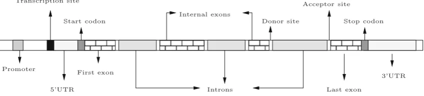
In prokaryotic organisms, the task of gene finding seems to be easier than in eukaryotics. In the former, most of the DNA sequence is coding for protein. Furthermore, each prokary-otic gene is a continuous stretch of coding bases, making the identification of these regions a feasible task. The genes of most eukaryotic organisms, on the other hand, are sep-arated by long stretches of intergenic DNA and their cod-ing fragments, called exons, are interrupted by non-codcod-ing ones, called introns. In addition to the exons and introns, the eukaryotic genes include a number of other elements, such as 5-UTR, 3-UTR and splicing (donor and acceptor) sites. The structure of a typical multi-exon eukaryotic gene is shown in Fig.1.
Fig. 1 Simplified structure of a multi-exon gene
[9,13–15,21,23,38,41,53] make use of similarity informa-tion between the genomic sequence and a fully annotated transcript sequence, such as cDNA, EST or protein, in order to accomplish the gene prediction task.
Recently, with the huge amount of newly sequenced genomes, new similarity-based methods are being success-fully applied in the task of gene prediction. In some ways different from traditional extrinsic methods, the so-called comparative-based methods[5,10,32,35–37,49], pioneered by Batzoglou et al. [4] with Rosetta, rely on similari-ties between regions of two or more unannotated genomic sequences in order to find the genes encoded in each of them. The main assumption of these methods is that the func-tional parts of the eukaryotic genomic sequences, the coding regions, tend to be more conserved than the non-functional ones. Finally, it is important to make reference to gene pre-diction tools that combine extrinsic and intrinsic informa-tion. This is the case, for example, ofAugustus- PPX[22], Twinscan[24],DoubleScan[33] andGenomeScan[52]. Despite the enormous progress made to date (see Brent and Guigó [6] and Sleator [43] for a survey on this topic), the gene identification problem remains an interesting subject of research.
Given the importance of genome comparison in obtaining information about these types of data, a number of heuris-tics algorithms aimed at constructing biologically meaning-ful alignments were developed [3,18,29,31,47]. In order to deal specifically with sequences whose conserved regions are intervened by unconserved ones, such as protein and prokaryotic gene sequences, Huang and Chao proposed in [20] the generalized global alignment. This type of alignment discriminates between conserved and unconserved regions by using the concept of difference blocks. Unfortunately, there are still situations where even the generalized global alignment cannot be applied in a meaningful way. This hap-pens, for example, when the sequences to be compared include highly conserved regions intervened by conserved and unconserved ones. This is exactly the case in stretches of eukaryotic genomic sequences that encode one or more genes. With the practical restrictions of the generalized global alignment, Huang and Brutlag describe in [19] an algorithm that computes an optimal alignment of two sequences by
using a set of multiple parameters with different levels of stringency.
We propose in this work a new type of alignment, called syntenic global alignment, jointly with an algorithm that, given two sequences, constructs a best syntenic global align-ment between them and calculates the associated value of similarity. This alignment can be seen as a generalization of the generalized global alignment where three types of blocks are taken into account, and the corresponding algo-rithm is a special case of that proposed by Huang and Brutlag.
In order to evaluate the applicability of our approach, the proposed alignment algorithm was used in the develop-ment of a new gene prediction tool calledExon_Finder2. Our program was tested on two different benchmarks that include several pairs of real human and mouse genomic sequences. The first benchmark includes 50 pairs of genomic sequences taken from two traditional datasets. The second benchmark includes 70 pairs of genomic sequences. These pairs were obtained by us taking as base the human chro-mosome sequences of the ENCODE project and their cor-responding annotation. The genes encoded in a number of sequences that constitute these benchmarks were correctly located by our approach.
This paper is organized as follows. In the next section we introduce the syntenic global alignment and show the recurrences that allow us to find an optimal alignment of this type. Details about the use of this algorithm as a tool to the gene prediction task are given in Sect.2.1. The experimental results are shown in Sect.3. In the final section we make some concluding remarks concerning this work.
2 Syntenic global alignment
the Smith–Waterman [44] algorithm identifies only a high-scoring similar region shared by the sequences (local align-ment).
In order to deal with sequences that have intermittent similarities, Huang and Chao proposed in [20] a variant of the global alignment calledgeneralized global alignment. In such work, the notion of difference block is introduced. Such a block includes residues that fall inside unconserved regions of the sequences that are being compared. With this new block, the task is to search for a best alignment of the input sequences allowing the use of gaps, matches, mismatches and differences. To this end, the authors suggest a dynamic pro-gramming algorithm that makes use of four different matri-ces:S,I,DandH. The first one is related to matches and mismatches. The matrices I and Ddeal with indels when comparing the sequences. Finally, the matrixHcorresponds to the difference block.
The generalized global alignment can be used to dis-tinguish between conserved and unconserved regions of pairs of sequences. Despite this practical advantage over the global and local alignments, the generalized global align-ment does not give good results when applied to a pair of sequences whose regions can be partitioned into highly conserved, conserved and unconserved, which is actually what occurs frequently in the real data. In order to fill this gap, we propose in this work a new type of alignment, calledsyntenic global alignment, that includes three types of blocks:
– highly conserved blocks: blocks where regions with a high degree of similarity are aligned;
– conserved blocks: blocks where regions with a low degree of similarity are aligned;
– unconserved blocks: blocks where regions with no simi-larity are aligned.
Given two sequencesX =x1x2. . .xm andY =y1y2. . .yn,
of lengthsmandn, respectively, a syntenic global alignment ofXandYincludes matches, mismatches and indels involv-ing symbols of X andY that fall inside highly conserved and conserved regions of these sequences. Additionally, it deals with symbols ofXandYthat compose regions of these sequences where no conservation is expected. An example of a syntenic global alignment is shown in Fig.2. Matches, mis-matches and indels inside highly conserved blocks (resp.(or) conserved blocks) are represented by columns with the sym-bols ‘|’, ‘/’, ‘-’ (resp. ‘:’, ‘\’, ‘∼’). The unconserved blocks are represented by the symbol ‘*’.
Letw(resp.w) be a scoring function that assigns real val-ues for pairs of characters lined up in highly conserved blocks (resp. conserved blocks). Additionally, letgandh (resp.g andh) be real values associated, respectively, with the first
Fig. 2 Example of a syntenic global alignment
and subsequent spaces in a gap of lengthl>1 inside a highly conserved block (resp. conserved block). Finally, letdbe a real value corresponding to a cost of each unconserved block. Given these definitions, the score of a syntenic global align-mentAis the sum of the values of each match, mismatch, gap and unconserved block in this alignment. With these defini-tions in mind, the problem we consider is the following: given two sequencesX =x1,x2, . . . ,xmandY =y1,y2, . . . ,yn,
find an optimal syntenic global alignment of X andY, that is, a syntenic global alignment of these sequences with a maximum score.
Like most of the alignment algorithms in the literature, the one proposed in this work is based on the dynamic program-ming approach. Given two sequences X andY, an optimal syntenic global alignment between these sequences can be found by making use of seven matricesH,S,S,I,I,Dand D, where:
(1) H[i][j]: stores the score of a best alignment between x1x2. . .xi andy1y2. . .yjending inside an unconserved
block;
(2) S[i][j](resp.S[i][j]): stores the score of a best align-ment betweenx1x2. . .xiandy1y2. . .yjending with the
symbolsxi andyj inside a highly conserved (resp.
con-served) block;
(3) I[i][j](resp.I[i][j]): stores the score of a best align-ment between x1x2. . .xi and y1y2. . .yj ending with
an insertion inside a highly conserved (resp. conserved) block;
(4) D[i][j](resp.D[i][j]): stores the score of a best align-ment between x1x2. . .xi and y1y2. . .yj ending with
a deletion inside a highly conserved (resp. conserved) block;
From the above definitions, the following recurrences can be used to compute the matricesH,S,S,I,I,DandD.
S[0][0] =0
S[0][0] =0
D[0][j] = D[0][j−1] −g(j >0) D[0][j] = D[0][j−1] −g(j>0)
H[i][j] =max ⎧ ⎪ ⎪ ⎪ ⎪ ⎪ ⎪ ⎪ ⎪ ⎪ ⎪ ⎨ ⎪ ⎪ ⎪ ⎪ ⎪ ⎪ ⎪ ⎪ ⎪ ⎪ ⎩
H[i−1][j] H[i][j−1] S[i−1][j] −d D[i−1][j] −d I[i−1][j] −d S[i][j−1] −d D[i][j−1] −d I[i][j−1] −d.
S[i][j] =w(xi,yj)+max
⎧ ⎪ ⎪ ⎪ ⎪ ⎪ ⎪ ⎪ ⎪ ⎨ ⎪ ⎪ ⎪ ⎪ ⎪ ⎪ ⎪ ⎪ ⎩
S[i−1][j−1] S[i−1][j−1] D[i−1][j−1] D[i−1][j−1] I[i−1][j−1] I[i−1][j−1] H[i−i][j−1].
I[i][j] =max
⎧ ⎪ ⎪ ⎪ ⎪ ⎪ ⎪ ⎪ ⎪ ⎨ ⎪ ⎪ ⎪ ⎪ ⎪ ⎪ ⎪ ⎪ ⎩
S[i][j−1] −(h+g) S[i][j−1] −(h+g) D[i][j−1] −(h+g) D[i][j−1] −(h+g) I[i][j−1] −g I[i][j−1] −g H[i][j−1].
D[i][j] =max
⎧ ⎪ ⎪ ⎪ ⎪ ⎪ ⎪ ⎪ ⎪ ⎨ ⎪ ⎪ ⎪ ⎪ ⎪ ⎪ ⎪ ⎪ ⎩
S[i−1][j] −(h+g) S[i−1][j] −(h+g) D[i−1][j] −g D[i−1][j] −g I[i−1][j] −(h+g) I[i−1][j] −(h+g) H[i−1][j].
S[i][j] =w(xi,yj)+max
⎧ ⎪ ⎪ ⎪ ⎪ ⎪ ⎪ ⎪ ⎪ ⎨ ⎪ ⎪ ⎪ ⎪ ⎪ ⎪ ⎪ ⎪ ⎩
S[i−1][j−1] S[i−1][j−1] D[i−1][j−1] D[i−1][j−1] I[i−1][j−1] I[i−1][j−1] H[i−1][j−1].
I[i][j] =max
⎧ ⎪ ⎪ ⎪ ⎪ ⎪ ⎪ ⎪ ⎪ ⎨ ⎪ ⎪ ⎪ ⎪ ⎪ ⎪ ⎪ ⎪ ⎩
S[i][j−1] −(h+g) S[i][j−1] −(h+g) D[i][j−1] −(h+g) D[i][j−1] −(h+g) I[i][j−1] −g I[i][j−1] −g H[i][j−1].
D[i][j] =max
⎧ ⎪ ⎪ ⎪ ⎪ ⎪ ⎪ ⎪ ⎪ ⎨ ⎪ ⎪ ⎪ ⎪ ⎪ ⎪ ⎪ ⎪ ⎩
S[i−1][j] −(h+g) S[i−1][j] −(h+g) D[i−1][j] −g D[i−1][j] −g I[i−1][j] −(h+g) I[i−1][j] −(h+g) H[i−1][j].
After filling out these matrices, the score of an optimal syn-tenic global alignment will correspond to the maximum value between S[m][n],S[m][n],D[m][n],D[m][n],I[m][n], I[m][n]and H[m][n]. An optimal syntenic alignment can be recovered by a traceback process. Starting from the entry where the optimal score is located, we proceed to the cell from which it was derived, and continue in this way until the first row or column of any matrix is reached.
The correctness of our approach is based on the prop-erties of overlapping problems and optimal substructure (at the blocks level) exhibited by the problem. This fact, jointly with the observation that every position[i][j]of each matrix can be computed looking at a constant number of previ-ous entries and taking the maximum for each case, ensure that an algorithm based on the above recurrence returns in polynomial time an optimal syntenic global alignment of the input sequences. Since our approach involves only the com-putation of 7mn values, one for each cell of the matrices S,S,D,D,I,IandH, an optimal syntenic global align-ment can be found inO(mn)time and space.
It is worthwhile to note that the results of our approach are strongly dependent on the scoring functionwand on the values ofgandh. Given the different degrees of conservation associated with the regions that align inside highly conserved and conserved blocks, the values ofgandhneed to be greater than the values ofgandh, respectively. Mismatches inside a highly conserved block must also have a greater cost than that associated with mismatches inside a conserved block. The syntenic global alignment of Fig. 2, for example, was calculated by means of a scoring function with these proper-ties. In fact, it is an optimal syntenic global alignment of the given sequences.
2.1 Application to the gene prediction problem
Several works in the literature state that the exons of eukary-otic genes tend to be more conserved than its introns, which in turn are more conserved than the intergenic regions. The dif-ferent levels of conservation between these regions lead to a direct application of the syntenic global alignment to the gene prediction problem. Given two orthologous sequences, the goal is to find an optimal syntenic global alignment between them. Segments of these sequences aligned inside highly conserved and conserved blocks of the resulting alignment would correspond to the exons and introns of the searched genes, respectively. The stretches aligned inside unconserved blocks would correspond to the intergenic regions of the input sequences.
and modifications we introduced to the recurrences in order to achieve better results in real-world instances of the gene prediction problem.
First of all, it is worthwhile to note that eukaryotic genes, with rare exceptions, start and end with an exon. Given this fact, the score of a best alignment ending in a conserved (intronic) region cannot be calculated from the score of a best alignment ending in an unconserved (intergenic) region of the input genomic sequences. In other words, a position(i,j)of the matrixScan only be calculated by choosing the maxi-mum betweenS[i−1][j−1],D[i−1][j−1],I[i−1][j−1] (extension of an intron) andS[i−1][j−1],D[i−1][j−1], I[i −1][j−1](beginning of an intron). For the same rea-son, the matricesI andDneed to be calculated by using the values from the matrices S,S,D,D,I and I. Like-wise, the score of a best alignment ending in an unconserved (intergenic) region cannot be calculated from the score of a best alignment ending in a conserved region (intron) of the two sequences. In this case, a position(i,j)of the matrixH can only be calculated by taking into account the values at positions(i−1,j)and(i,j −1)of the matrices H,S,D andI.
Some properties related to the splicing sites can also be helpful in the gene prediction task. It is well known that most real acceptor (resp. donor) sites include the dinucleotidesAG (resp.GT). Taking this into account, the score of a best align-ment ending in the first position of a possible exon (resp. intron) can only be calculated in the presence of the din-ucleotidesAG (resp.GT) in both sequences. Furthermore, given the importance of the splicing sites during the protein synthesis process, they tend to present a high degree of con-servation. This allows us to consider only the matrixSto fill the matricesS,DandI. In the same way, only the matrix S will be used to fill the matricesS,DandI. This means that we are not interested in alignments where the corre-sponding splicing sites (one from each sequence) do not align exactly.
Finally, it is also well known that most true start sites (resp. stop sites) include the codonATG(resp.TAA,TAG, TGA). Consequently, the score of a best alignment ending in the first (resp. last) position of the searched gene can only be calculated in the presence of the codonATG(resp.TAA, TAG,TGA) in both sequences.
Given the large number of false-positive splicing sites where all the dinucleotides AG/GT are taken as poten-tial acceptor/donor sites, a preprocessing step of the input sequences becomes necessary in order to identify the most promising ones. In other words, in this step we are search-ing for dinucleotides AG/GT with high probability (log-likelihood score) of being true splicing sites. Given a genomic sequence, the log-likelihood scorePof each possible splic-ing site can be calculated ussplic-ing the conditional probability matrices described by Salzberg in [40]. These values are thus
H
GT AG
ATG TAG
ATG TAG ATG
TAG S
I
D
S’
I’
D’
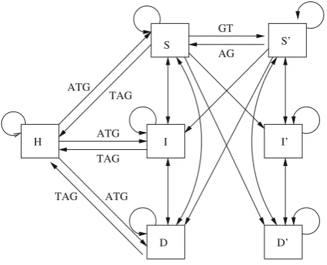
Fig. 3 Schematic representation of the filling of matrices
S,S,D,D,I,IandH
taken into account in the filling of the matricesS,S,D,D,I andI. This is done by considering the value from the matrix S(resp.S) as a possible maximum to calculate the value of a position(i,j)of the matricesS,DandI (resp.S,Dand I) only ifP(s[i..i+1])andP(t[j..j+1])are greater than a given thresholdT.
The observations above and all the restrictions to the filling of the matricesS,D,I andH imposed by them are repre-sented in Fig. 3, where each square represents a dynamic programming matrix. A directed edge between two squares means that the matrix represented by the square on the end point can only be filled by using the values from the matrix represented by the square at the start point of the edge. Finally, labels in the directed edges represent the need for some specific site in the sequences.
3 Experimental results
We used the above ideas in the implementation of a new comparative-based gene prediction tool. Our program, called Exon_Finder2,1takes as input two sequences in FASTA for-mat and returns the locations of the exons predicted in these sequences. These locations correspond to the start and end positions of each highly conserved block in the correspond-ing syntenic global alignment.
In order to evaluate our approach,Exon_Finder2 was tested on two benchmarks that include a number of pairs of single gene sequences from human and mouse. The first benchmark was used to compare our approach with some other gene finding programs. In this case, the values of the parameters used by our program were estimated in accor-dance with the number and length of exons in each pair of sequences. The second benchmark was used to assess the significance of our approach on a real world situation, in which the biologist would not know how to select the parame-ters properly. Details about these benchmarks and the results achieved by our approach will be given in Sects.3.1and3.2 respectively.
To assess the accuracy of the programs, we made use of the following measures introduced by Burset and Guigó in [8]. In what follows, the term “predicted” will refer to the informa-tion about the genes retrieved by the programs, whereas the terms “annotated” and “really” will refer to the information about the genes as found in the databases.
(1) Specificity at the nucleotide level (Spn= TPTP+FP): pro-portion of nucleotides predicted as coding that are really coding;
(2) Sensitivity at the nucleotide level (Snn= TPTP+FN): pro-portion of really coding nucleotides correctly predicted as coding;
(3) Specificity at the exon level (Spe= NCENPE): proportion of predicted exons that match an annotated exon;
(4) Sensitivity at the exon level (Sne = NCENAE): proportion of annotated exons in the input sequence that have been correctly predicted.
At the nucleotide level, the quantity approximate correla-tion, AC, defined as
AC= 1 2
TP TP+FN+
TP TP+FP+
TN TN+FP+
TN TN+FN
−1
has been introduced to summarize sensitivity and specificity in a single measure. At the exon level, the average Av =
(Spe+Sne)/2 is used instead.
1This name was chosen in reference to other (similarity-based) gene
prediction tool developed by the authors, calledExon_Finder1, whose details can be seen in [2].
In the above definitions, TP (true positives) is the num-ber of really coding nucleotides correctly predicted as cod-ing, TN (true negatives) represents the number of really non-coding nucleotides correctly predicted as non-coding, FP (false positives) is the number of really non-coding nucleotides incorrectly predicted as coding and FN (false negatives) is the number of really coding nucleotides incor-rectly predicted as non-coding. On the level of complete exons, one defines NCE as the number of correctly predicted exons, NPE as the number of predicted exons and NAE as the number of annotated exons. Here, like Burset and Guigó, we consider an exon as correctly predicted when both its limits are identical to the limits of an annotated exon in the input sequences. About the predicted exons whose limits are dif-ferent from the limits of an annotated exon, we will refer to them as mispredicted exons (when there is some intersection between the predicted exon and an annotated exon) or over-predicted exons (when there is no intersection between the predicted exon and an annotated exon).
3.1 Comparison with previous approaches
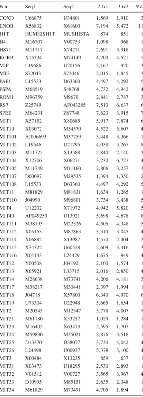
Our approach was first evaluated on a benchmark whose sequences were taken from the dataset used by Jareborg et al. [37] in the training and testing of theSGP- 2gene prediction program (IMOG and SCIMIT dataset). All the genes encoded in each of these sequences were evaluated experimentally and the sequences themselves have been used as a standard set to the evaluation of earliest comparative-based gene predic-tion programs. Detailed informapredic-tion about these sequences is shown on Table1.
For a better insight into the accuracy of our program, the results of Exon_Finder2 were compared with those achieved by the other three comparative-based gene predic-tion tools, namely Utopia[5],Progen[35] andAgenda [46]. All of these programs were run with their suggested default parameters.
The average values of specificity and sensitivity achieved by our program, at both nucleotide and exon levels, are shown in the first line of Table2.
Table 1 Additional information about the first dataset
Pair Seq1 Seq2 L G1 L G2 N E
COXD U66875 U34801 1,569 1,910 3
ENOB X56832 X61600 7,194 5,472 11
H1T HUMHISH1T MUSHISTA 874 851 1
H4 M16707 V00753 1,098 968 1
HS71 M11717 X74271 2,691 5,918 1
KCRB X15334 M74149 4,200 4,521 7
MIF L19686 U20156 2,167 920 3
MT3 S72043 S72046 2,015 1,845 3
PAP1 L15533 D63360 4,497 4,292 5
PSPA M68519 S48768 4,732 4,942 4
ROM1 M96759 M9670 2,841 2,787 3
RS7 Z25749 AF043285 7,513 6,637 6
SPEE M64231 Z67748 7,623 3,915 7
MIT1 X57152 X80685 5,917 7,874 6
MIT10 X03072 M34570 4,522 5,607 4
MIT101 AJ006693 M37759 3,448 3,366 1 MIT102 L19546 U21795 4,038 5,267 8 MIT103 M11725 X13588 2,840 2,140 2 MIT104 X12706 X06271 3,230 6,727 4 MIT105 M11749 M11160 2,806 3,257 3 MIT107 D00097 M29535 1,394 1,350 2 MIT108 L15533 D63360 4,497 4,292 5
MIT11 M81829 M81831 1,634 1,265 1
MIT110 J04990 M96801 3,734 3,438 5
MIT4 U12202 X71972 4,942 5,820 5
MIT40 AF049259 U13921 5,698 4,678 8 MIT111 M38193 M22526 4,505 4,348 5 MIT112 X05153 M87863 3,310 3,045 4 MIT114 X06882 X13987 1,570 2,404 2 MIT115 X74322 U60528 2,609 5,416 3
MIT116 X04143 L24429 1,675 949 4
MIT12 Y00508 J04192 2,100 1,574 1
MIT13 X65921 L33715 2,016 2,850 4
MIT14 M28638 M73741 4,206 4,181 3
MIT17 M38217 M30441 2,397 1,994 1
MIT18 J04718 X57800 6,340 4,970 6
MIT19 U73304 U22948 5,665 1,654 1
MIT2 M20543 M12347 3,778 4,007 7
MIT21 M61180 X53257 1,029 1,284 1
MIT23 M16405 X63473 2,595 1,707 1
MIT24 M59830 M35021 2,876 3,518 1
MIT25 D13370 D38077 3,730 4,042 4
MIT26 L24498 U00937 5,378 3,100 4
MIT3 X60484 X13235 859 637 1
MIT31 X03473 U18295 2,530 2,893 1
MIT32 V01512 V00727 3,565 3,967 4
MIT33 D10995 M85151 2,635 2,348 1
MIT34 M61829 M73491 4,705 1,894 1
Table 1 continued
Pair Seq1 Seq2 L G1 L G2 N E
MIT36 M96264 U41282 4,286 4,023 11
MIT39 L19686 U20156 2,167 920 3
Pair Pair identification, Seq1 accession field of the first genomic sequence,Seq2accession field of the second genomic sequence,LG1
length of the first genomic sequence,LG2length of the second genomic sequence,NEnumber of exons
Table 2 Average values of specificity and sensitivity, in both nucleotide and exon levels, achieved by the evaluated tools
Tool Spn Snn AC Spe Sne Av
Exon_Finder2 0.85 0.93 0.84 0.54 0.57 0.56
Agenda 0.97 0.82 0.84 0.68 0.62 0.65
ProGen 0.95 0.98 0.94 0.38 0.66 0.76
Utopia 0.86 0.98 0.89 0.38 0.52 0.45
outperformsProgenwith a 16 % improvement of the exon specificity, but in general it is less accurate thanProgenand Agendaat the exon level.
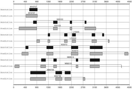
The low value of specificity obtained by our approach at the nucleotide level is mainly due to the number of nucleotides that were incorrectly predicted as coding at the boundaries of the annotated exons in the sequences, where the rate of conservation is relatively high when compared with that presented by the intronic and intergenic regions. This problem becomes more evident when the first and last exons of the genes are considered. The pair H4, which includes the sequences M16707 and V00753, is a useful example of this drawback. Both of these sequences encode a gene with a sin-gle exon. They start at the positions 613 and 258 and end at the positions 924 and 569 of M16707 and V00753, respectively. The single-exon gene predicted byExon_Finder2starts at the positions 477 of M16707 and 115 of V00753 and ends at the correct positions 924 and 569 of these sequences. Look-ing at the alignment of M16707 and V00753 constructed by our program, we can see a high degree of conservation at the 5-UTR regions of the target genes (Fig.4). This fact, in conjunction with the presence of a start codon (ATG) on both sequences, leads to the prediction of genes starting about 140 nucleotides earlier than their real start positions. Fig-ure5shows a graphical representation of some mispredicted exons spanning out of the intergenic and intronic regions of the sequences M16707 and X05153.
Fig. 4 A stretch of the syntenic global alignment of the sequences M16707 and V00753 that reveals a high degree of conservation on the boundaries of their single-exon genes.PStP Predicted start position,
TStPtrue start position
A useful example of this drawback is the pair that includes the sequences M68519 and S48768. In each one of these sequences, two additional exons that do not have intersection with the annotated ones were overpredicted by our program. Both of these exons are located outside the corresponding genes. This fact leads to a unsatisfactory value of speci-ficity of Exon_Finder2 at the exon level. Only 54 % of the predicted exons are in accordance with annotated exons. Figure5shows a graphical representation of some overpre-dicted exons inside the intergenic regions of the sequences L15533, M68519, M96759 and X03072.
Regarding the sensitivity of our approach, only 57 % of annotated exons were correctly predicted by our tool. The large majority of missed exons correspond to small and unconserved ones. This occurs, for example, with the first exons in the sequences M96264 and U41282. Both of them are small exons, and the corresponding global pairwise align-ment shows a number of consecutive spaces.
3.2 Automatic parameter setting
In addition to the tests whose results were detailed in the pre-vious section, other experiments were made in order to best evaluate the practical usefulness of our approach. To this
0 450 900 1350 1800 2250 2700 3150 3600 4050 4500
0 450 900 1350 1800 2250 2700 3150 3600 4050 4500
M16707
M16707
X05153
X05153
L15533
L15533
X03072
X03072
M68519
M68519
M96759
M96759
end, we create a benchmark from the human chromosome sequences of the ENCODE (ENCyclopedia of DNA ele-ments) project [11]. These sequences span 1 % of the human genome sequence and the corresponding annotation [16] has been used as the “golden standard” to assess the performance of computational methods developed for the identification of functional elements.
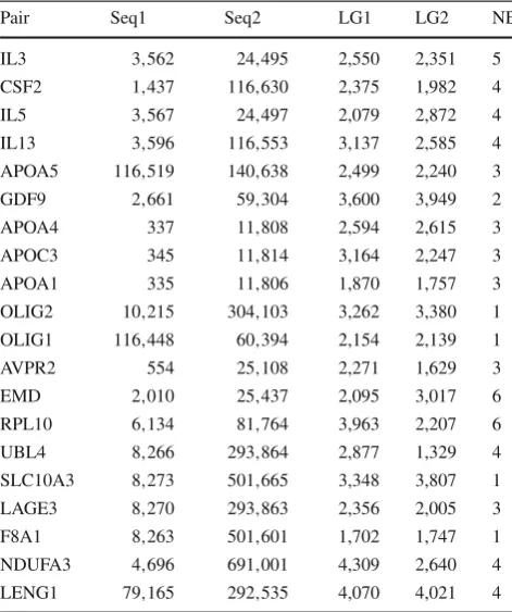
The new pairs of sequences used as input of our program were constructed in the following way. From the sequences ENm001, ENm002, ENm003, ENm004, ENm005, ENm006 and ENm007, we chose all the annotated (VEGA-Known) protein-coding genes with maximum length 5,000bp and no alternative splicing. At the second step, a homologous for each of these genes was taken from the HomoloGene Data-base [48]. To each sequence obtained, we left 100 bp of inter-genic region at their 5and 3side. A total of 20 pairs were obtained following these criteria. Details of each one of these pairs can be viewed in Table3.
Different from the previous round of tests, when the para-meters of the program were tuned manually, with this new benchmark it was done automatically by means of a genetic algorithm. The quality of the results on each round of this algorithm was evaluated based on the correct positions of the exons on the homologous sequence. Our idea was to test an automatic parameter choice, which would probably be used
Table 3 Additional information about the second dataset
Pair Seq1 Seq2 LG1 LG2 NE
IL3 3,562 24,495 2,550 2,351 5
CSF2 1,437 116,630 2,375 1,982 4
IL5 3,567 24,497 2,079 2,872 4
IL13 3,596 116,553 3,137 2,585 4
APOA5 116,519 140,638 2,499 2,240 3
GDF9 2,661 59,304 3,600 3,949 2
APOA4 337 11,808 2,594 2,615 3
APOC3 345 11,814 3,164 2,247 3
APOA1 335 11,806 1,870 1,757 3
OLIG2 10,215 304,103 3,262 3,380 1 OLIG1 116,448 60,394 2,154 2,139 1
AVPR2 554 25,108 2,271 1,629 3
EMD 2,010 25,437 2,095 3,017 6
RPL10 6,134 81,764 3,963 2,207 6
UBL4 8,266 293,864 2,877 1,329 4
SLC10A3 8,273 501,665 3,348 3,807 1 LAGE3 8,270 293,863 2,356 2,005 3
F8A1 8,263 501,601 1,702 1,747 1
NDUFA3 4,696 691,001 4,309 2,640 4 LENG1 79,165 292,535 4,070 4,021 4
PairPair identification,Seq1geneID of the first genomic sequence,
Seq2geneID of the second genomic sequence, LG1 length of the first genomic sequence,LG2length of the second genomic sequence,
NEnumber of exons
Table 4 Average values of specificity and sensitivity, in both nucleotide and exon levels, achieved byExon_Finder2on the second benchmark
Tool Spn Snn AC Spe Sne Av
Exon_Finder2 0.88 0.92 0.87 0.53 0.70 0.62
by a biologist in a real-world application. In this case, given a sequence where one gene exists, the first step would be to search for a homologous of it and run our program using in a useful way some information concerning the homologous gene.
The values of specificity and sensitivity achieved in this case are presented on Table4.
As it can be seen, the results of Exon_Finder2on this round of tests are a little bit better than that obtained with the first benchmark. From a total of 65 real exons, 46 were correctly predicted by our approach. Moreover, from the 86 exons predicted by our approach, 25 have no intersection with a real exon. From these, 13 are located inside the intronic regions of the input sequences and 12 are located outside the gene. Interestingly, all but three of the 12 exons overpredicted outside the genes are located at their 3-intergenic regions. About the 13 exons overpredicted inside the intronic regions of the input sequences, they correspond to small exon of average length 26 bp.
These further results show that our approach can be suc-cessfully used in the task of gene finding, especially if com-bined with modifications to incorporate biological informa-tion and with the use of an automatic tool to tune the various parameters involved.
4 Discussion
Despite its practical importance and the number of meth-ods developed to date, the gene identification remains an open and interesting problem. Given the increasing number of homologous sequences in the databases and the assump-tion that the exons tend to be more conserved than the introns inside a genome, comparative-based gene prediction pro-grams start to be extensively used in the task of gene identifi-cation. In this work we presented a new gene prediction tool, whose implementation is based on a new type of alignment proposed by us and called syntenic global alignment.
corre-sponding algorithm was used in the development of a new tool to the gene prediction problem calledExon_Finder2.
Regarding the first experimental results, the outcomes were quite promising considering the fact that our method uses only information about the different rates of conserva-tion related to the regions of the input sequences. The main drawback of our approach is due to the existence of well conserved regions outside the target genes. This leads to a number of overpredicted exons and additional bases incor-rectly identified as coding at the 5-UTR and 3-UTR regions of the annotated genes and, consequently, to a low value of specificity and sensitivity at the exon level. Further tests were performed with the parameters being automatically tuned by a genetic algorithm. Similar results for specificity and sensi-bility were obtained, showing that our approach can be suc-cessfully used in the task of gene finding.
One way to obtain better results with the proposed tool in the context of the gene prediction problem is to use statistical information that can give better insights into the localization of the real start and stop codons in the sequences. Additional information, such as reading frame and codon usage, can also be incorporated into theExon_Finder2in order to improve its results. These works are in progress in the hope that better values of specificity and sensitivity at both the nucleotide and the exon level can be achieved in the future. The study of other applications to the syntenic global alignment is also a promising object of research.
References
1. Abbasi O, Rostami A, Karimian G (2011) Identification of exonic regions in DNA sequences using cross-correlation and noise sup-pression by discrete wavelet transform. BMC Bioinforma. doi:10. 1186/1471-2105-12-430
2. Adi SS, Ferreira CE (2003) A gene prediction algorithm using the spliced alignment problem. São Paulo, Instituto de Matemática e Estatística-USP. RT-MAC-2003-04
3. Agrawal A, Huang XG (2009) Pairwise statistical significance of local sequence alignment using sequence-specific and position-specific substitution matrices. IEEE ACM Trans Comput Biol Bioinforma 8(1):194–205. doi:10.1109/TCBB.2009.69
4. Batzoglou S, Pachter L, Mesirov JP, Berger B, Lander ES (2000) Human and mouse gene structure: comparative analysis and appli-cation to exon prediction. Genome Res 10(7):950–958. doi:10. 1101/gr.10.7.950
5. Blayo P, Rouzé P, Sagot M-F (2003) Orphan gene finding: an exon assembly approach. Theor Comput Sci 290(3):1407–1431. doi:10. 1016/S0304-3975(02)00043-9
6. Brent MR, Guigó R (2004) Recent advances in gene structure pre-diction. Curr Opin Struct Biol 14(3):264–272. doi:10.1016/j.sbi. 2004.05.007
7. Burge C, Karlin S (1997) Prediction of complete gene structures in human genomic DNA. J Mol Biol 268(1):78–94. doi:10.1006/ jmbi.1997.0951
8. Burset M, Guigó R (1996) Evaluation of gene structure prediction programs. Genomics 34(3):353–367. doi:10.1006/geno.1996.0298
9. Chen M, Manley JL (2009) Mechanisms of alternative splicing regulation: insights from molecular and genomics approaches. Nat Rev Mol Cell Biol 10(11):741–754. doi:10.1038/nrm2777 10. Dewey C, Wu JQ, Cawley S, Alexandersson M, Gibbs R, Pachter
L (2004) Accurate identification of novel human genes through simultaneous gene prediction in human mouse and rat. Genome Res 14(4):661–664. doi:10.1101/gr.1939804
11. The ENCODE Project Consortium (2004) The ENCODE (ENCy-lopedia Of DNA Elements) project. Science 306(5696):636–640. doi:10.1126/science.1105136
12. Fickett JW (1982) Recognition of protein coding regions in DNA sequences. Nucleic Acids Res 10(17):5303–5318. doi:10.1093/ nar/10.17.5303
13. Florea L, Hartzell G, Zhang Z, Rubin GM, Miller W (1998) A computer program for aligning a cDNA sequence with a genomic sequence. Genome Res 8(9):967–974
14. Gelfand MS, Mironov AA, Pevzner PA (1996) Gene recognition via spliced sequence alignment. Proc Natl Acad Sci USA 93(17):9061– 9066. doi:10.1073/pnas.93.17.9061
15. Gotoh O (2008) A space-efficient and accurate method for mapping and aligning cDNA sequences onto genomic sequence. Nucleic Acids Res 36(8):2630–2638. doi:10.1093/nar/gkn105
16. Harrow H et al (2006) GENCODE: producing a reference annota-tion for ENCODE. Genome Biol. doi:10.1186/gb-2006-7-s1-s4 17. Harrow J, Nagy A, Reymond A, Alioto T, Patthy L, Antonarakis
SE, Guigó R (2009) Identifying protein-coding genes in genomic sequences. Genome Biol. doi:10.1186/gb-2009-10-1-201 18. Huang W, Umbach DM, Li LP (2006) Accurate anchoring
align-ment of divergent sequences. Bioinformatics 22(1):29–34. doi:10. 1093/bioinformatics/bti772
19. Huang X, Brutlag DL (2007) Dynamic use of multiple parameter sets in sequence alignment. Nucleic Acids Res 35:678–686. doi:10. 1093/nar/gkl1063
20. Huang X, Chao K-M (2003) A generalized global align-ment algorithm. Bioinformatics 19(2):228–233. doi:10.1093/ bioinformatics/19.2.228
21. Kapustin Y, Souvorov A, Tatusova T, Lipman D (2008) Splign: algorithms for computing spliced alignments with identification of paralogs. Biol Direct. doi:10.1186/1745-6150-3-20
22. Keller O, Kollmar M, Stanke M, Waack S (2011) A novel hybrid gene prediction method employing protein multiple sequence alignments. Bioinformatics 27(6):757–763. doi:10.1093/ bioinformatics/btr010
23. Keller O, Odronitz F, Stanke M, Kollmar M, Waack S (2008) Sci-pio: using protein sequences to determine the precise exon/intron structures of genes and their orthologs in closely related species. BMC Bioinforma. doi:10.1186/1471-2105-9-278
24. Korf I, Flicek P, Duan D, Brent MR (2001) Integrating genomic homology into gene structure prediction. Bioinformatics 17(Suppl. 1):S140–S148
25. Krogh A (1997) Two methods for improving performance of an HMM and their application for gene finding. Proc Int Conf Intell Syst Mol Biol 5:179–186
26. Krogh A (2000) Using database matches with HMMGene for auto-mated gene detection in Drosophila. Genome Res 10(4):523–528. doi:10.1101/gr.10.4.523
27. Krogh A, Mian IS, Haussler D (1994) A hidden Markov model that finds genes inE. coliDNA. Nucleic Acids Res 22(22):4768–4778. doi:10.1093/nar/22.22.4768
28. Kulp D, Haussler D, Reese MG, Eeckman FH (1996) A generalized hidden Markov model for the recognition of human genes in DNA. Proc Int Conf Intell Syst Mol Biol 4:134–142
30. Mathé C, Sagot M-F, Schiex T, Rouzé P (2002) Current methods of gene prediction their strengths and weaknesses. Nucleic Acids Res 30(19):4103–4117. doi:10.1093/nar/gkf543
31. Morgenstern B, Frech K, Dress A, Werner T (1998) Dialign: finding local similarities by multiple sequence alignment. Bioinformatics 14(3):290–294. doi:10.1093/bioinformatics/14.3.290
32. Morgenstern B, Rinner O, Abdeddaïm S, Haase D, Mayer KF, Dress AW, Mewes HW (2002) Exon discovery by genomic sequence alignment. Bioinformatics 18(6):777–787. doi:10.1093/ bioinformatics/18.6.777
33. Meyer IM, Durbin R (2002) Comparative ab initio prediction of gene structures using pair HMMs. Bioinformatics 18(10):1309– 1318. doi:10.1093/bioinformatics/18.10.1309
34. Needleman SB, Wunsch CD (1970) A general method applicable to the search for similarities in the amino acid sequence of two proteins. J Mol Biol 48(3):443–453
35. Novichkov PS, Gelfand MS, Mironov AA (2001) Gene recognition in eukaryotic DNA by comparison of genomic sequences. Bioin-formatics 17(11):1011–1018. doi:10.1093/bioinBioin-formatics/17.11. 1011
36. Pachter L, Alexandersson M, Cawley S (2002) Applications of generalized pair hidden Markov models to alignment and gene finding problems. J Comput Biol 9(2):389–399. doi:10.1089/ 10665270252935520
37. Parra G, Agarwal P, Abril JF, Wiehe T, Fickett JW, Guigó R (2003) Comparative gene prediction in human and mouse. Genome Res 13(1):108–117. doi:10.1101/gr.871403
38. Pirola Y, Rizzi R, Picardi E, Pesole G, Della Vedova G, Bonizzoni P (2012) PIntron: a fast method for detecting the gene structure due to alternative splicing via maximal pairings of a pattern and a text. BMC Bioinforma. doi:10.1186/1471-2105-13-S5-S2
39. Roitberg MA, Astakhova TV, Gelfand MS (1997) A combinatorial algorithm for highly specific recognition of protein-coding regions in higher eukaryotic DNA sequences. Mol Biol 31(1):18–23 40. Salzberg SL (1997) A method for identifying splice sites and
translational start sites in eukaryotic mRNA. Comput Appl Biosci 13(4):365–376
41. She R, Chu JS, Uyar B, Wang J, Wang K, Chen NS (2011) gen-BlastG: using BLAST searches to build homologous gene models. Bioinformatics 27(15):2141–2143. doi:10.1093/bioinformatics/ btr342
42. Shepherd JCW (1981) Method to determine the reading frame of a protein from the purine/pyrimidine genome sequence and its possi-ble evolutionary justification. Proc Natl Acad Sci USA 78(3):1596– 1600. doi:10.1073/pnas.78.3.1596
43. Sleator RD (2010) An overview of the current status of eukaryote gene prediction strategies. Gene 461(1–2):1–4. doi:10.1016/j.gene. 2010.04.008
44. Smith TF, Waterman MS (1981) Identification of common mole-cular subsequences. J Mol Biol 147(1):195–197. doi:10.1016/ 0022-2836(81)90087-5
45. Stanke M, Waack S (2003) Gene prediction with a hidden Markov model and a new intron submodel. Bioinformatics 19(Suppl. 2):ii215–ii225. doi:10.1093/bioinformatics/btg1080
46. Taher L, Rinner O, Garg S, Sczyrba A, Morgenstern B (2004) AGenDA: gene prediction by cross-species sequence comparison. Nucleic Acids Res 32:W305–W308. doi:10.1093/nar/gkh386 47. Tatusova TA, Madden TL (1999) BLAST 2 Sequences, a new tool
for comparing protein and nucleotide sequences. FEMS Microbiol Lett 174(2):247–250. doi:10.1111/j.1574-6968.1999.tb13575.x 48. Wheeler DL, Church DM, Federhen S, Lash AE, Madden TL,
Pontius JU, Schuler GD, Schriml LM, Sequeira E, Tatusova TA, Wagner L (2003) Database resources of the National Center for Biotechnology. Nucleic Acids Res 31(1):28–33. doi:10.1093/nar/ gkg033
49. Wu J, Haussler D (2006) Coding exon detection using compara-tive sequences. J Comput Biol 13(6):1148–1164. doi:10.1089/cmb. 2006.13.1148
50. Winters-Hilt S, Baribault C (2012) A metastate HMM with appli-cation to gene structure identifiappli-cation in eukaryotes. Eurasip J Adv Signal Process. doi:10.1155/2010/581373
51. Xu Y, Einstein JR, Mural RJ, Shah M, Uberbacher EC (1994) An improved system for exon recognition and gene modeling in human DNA sequences. Proc Int Conf Intell Syst Mol Biol 2:376–384 52. Yeh R-F, Lim LP, Burge CB (2001) Computational inference of
homologous gene structures in the human genome. Genome Res 11(5):803–816. doi:10.1101/gr.175701