An Improved Artificial Bee Colony Algorithm with Elite-Guided Search Equations

(1)

An Improved Artificial Bee Colony Algorithm

with Elite-Guided Search Equations

Zhenxin Du1,2, Dezhi Han1, Guangzhong Liu1, Kun Bi1, and Jianxin Jia1

1

College of Information Engineering, Shanghai Maritime University,

Shanghai 201306, China [email protected], dzhan, gzhliu,[email protected],

[email protected] 2

School of Computer Information Engineering, Hanshan Normal University,

Chaozhou 521041, China [email protected]

Abstract. ABC elite, a novel artificial bee colony algorithm with elite-guided search equations, has been put forward recently, with relatively good performance com-pared with other variants of artificial bee colony (ABC) and some non-ABC meth-ods. However, there still exist some drawbacks in ABC elite. Firstly, the elite solu-tions employ the same equation as ordinary solusolu-tions in the employed bee phase, which may easily result in low success rates for the elite solutions because of rela-tively large disturbance amplitudes. Secondly, the exploitation ability of ABC elite is still insufficient, especially in the latter half of the search process. To further improve the performance of ABC elite, two novel search equations have been pro-posed in this paper, the first of which is used in the employed bee phase for elite so-lutions to exploit valuable information of the current best solution, while the second is used in the onlooker bee phase to enhance the exploitation ability of ABC elite. In addition, in order to better balance exploitation and exploration, a parameterPo is introduced into the onlooker bee phase to decide which search equation is to be used, the existing search equation of ABC elite or a new search equation proposed in this paper. By combining the two novel search equations together with the new parameterPo, an improved ABC elite (IABC elite) algorithm is proposed. Based on experiments concerning 22 benchmark functions, IABC elite has been compared with some other state-of-the-art ABC variants, showing that IABC elite performs significantly better than ABC elite on solution quality, robustness, and convergence speed.

Keywords:artificial bee colony, search equations, exploration ability, exploitation ability.

1. Introduction

(2)

colony (ABC) algorithm has shown its superior performance in dealing with optimization problems [13], such as the flow shop scheduling problem [22], filter design problem [4], and vehicle routing problem [26].

However, ABC also suffers from slow convergence speed and easily being trapped by local optimum. This is mainly caused by its solution search equations, which is good at exploration but poor at exploitation [1, 5, 11, 21, 28]. In fact, the exploration and the ex-ploitation contradict each other. In order to achieve the excellent performance in solving optimization problems, the main challenge is how to maintain a delicate balance between the exploration and exploitation during the search process [5], and numerous ABC vari-ants have been proposed to improve ABC’s performance in this respect. Zhu et al. [28] proposed a gbest-guided ABC (GABC) to exploit the information of the global best in-dividual (gbest). In the ABC/best/1 algorithm [10], the information ofgbestis also used to enhance the exploitation ability of ABC. Wang et al. [27] proposed a multi-strategy ensemble ABC algorithm, which employs three distinct search equations to form a strat-egy pool and adaptively choose one of them in different search stratstrat-egy, thus the balance between exploration and exploitation can be maintained.

Recently, Cui et al. [5] proposed an artificial bee colony algorithm (the ABC elite) with two novel search equations. One search equation incorporates the beneficial infor-mation of elite solutions, which is applied to the employed bee phase, the other one not only exploits the valuable information of the elite solutions, but also employs that of the current best solution used in the onlooker bee phase. Furthermore, the ABC elite is embedded into depth-first framework to form a new variant of ABC, the DFSABC elite. Experimental results show that ABC-elite and DFSABC elite are very effective compared with other recently proposed ABC variants.

However, there still exist some drawbacks in the ABC elite/DFSABC elite. Firstly, in the employed bee phase of ABC elite, the elite solutions employ the same equation as ordinary solutions, easily resulting in the low success rate for the elite solutions because of relatively large disturbance amplitude. In the search equation of ABC elite, a candidate solution can be treated as the lead individual to explore the search space and produced by adding a scaled disturbance vector to a base vector. But we can draw inspiration from many EAs that the better the fitness value is, the smaller the disturbance amplitude is [3, 17–20, 24]. In a word, the disturbance of ordinary and elite solutions should be treated in a different way. Secondly, in the onlooker bee phase in ABC elite, the exploitation ability of ABC elite is still insufficient, especially in the latter half stage of a search process. To balance the exploitation and exploration ability, the search equation in the onlooker bee phase of ABC elite uses the difference betweengbestand a randomly selected ordinary individualXk as a disturbance vector, which is suitable for the ABC elite to maintain a

good balance between exploration and exploitation in the early stage of a search process, but easily leads to the insufficiency of exploitation ability in the latter half stage of a search process, because the ratio between exploration and exploitation is not constant. Generally speaking, EAs focus on exploration at the early stage and focus on exploitation at the latter half stage, which can also be seen in some other EAs [25].

(3)

the current best solution. Secondly, a novel search equation is proposed in the onlooker bee phase of ABC elite to further enhance the exploitation ability of ABC elite. In addi-tion, in order to obtain a better balance between exploitation and exploraaddi-tion, a parameter Pois used in the onlooker bee phase to choose a search equation between the original

one of ABC elite or the newly-proposed one. The simplicity of ABC elite is maintained in the proposed IABC elite. Moreover, the experiment results concerning 22 benchmark functions have demonstrated its effectiveness in solving complex numerical optimization problems when compared with the ABC elite, DFSABC elite and other ABC variants.

The rest of this paper is organized as follows. In Section 2, the original ABC algorithm is presented. In Section 3, the most recently developed ABC variants, the ABC elite al-gorithm, is reviewed, which is the basis of the proposed algorithm IABC elite. In Section 4, the IABC elite algorithm is proposed based on the two novel solution search equations (i.e., the Eq.(12) and Eq. (13)) and the new introduced search equation selective probabil-ityPo. Section 5 presents and discusses the experimental results. Finally, the conclusion

is drawn in Section 6.

2. The original ABC Algorithm

Inspired by the waggle dancing and foraging behaviors of honey bee colonies, the ABC algorithm has been developed. The basic ABC algorithm consists of four sequentially realized phases, i.e. the initialization, the employed bee, the onlooker bee and the scout bee. After the initialization phase, the ABC turns into a loop of the employed bee phase, onlooker bee phase and scout bee phase until the termination condition is satified. The details of each phase are described as follows:

Initialization phase: At the beginning of the ABC, the initial food sources are gen-erated randomly according to Eq. (1).

Xi,j=XjL+randj(XjU−X L

j) (1)

wherei={1,2, ..., SN},j ={1,2, ..., D},SN is the number of food sources, and SN is equal to the number of employed bees and onlooker bees.Dis the dimensionality (variables) of the search space.XL

j andXjU are the lower and upper bounds of thejth

variable respectively.randjis a random real number in range of [0,1]. Then, the fitness

values of the food sources are calculated by Eq. (2).

f iti= ₁₊_f1₍_Xi₎,f(Xi)≥0

f iti= 1+|f(Xi)|, f(Xi)<0

(2)

wheref iti is the fitness value of theith food sourceXi, andf(Xi)is the objective

function value of food sourceXi for the optimization problem. In addition, parameter

limitshould be determined and the parameter counter, which records the number of unsuccessful updates, is set to 0 for each food source.

Employed bee phase: Each employed bee will fly to a distinct food source and try to find out a candidate food source in the neighborhood of the corresponding parent food source by using Eq. (3).

(4)

wherei,kare picked up from{1,2, ..., SN}randomly,jis randomly selected from

{1,2, ..., D},Vi,jis thejth dimension of the ith candidate food source (new solution).

Xi,jis thejth dimension of theith food source;Xk,jis thejth dimension of thekth food

source,φi,jis a random real number in the range of [-1,1].

After creating a new food source, the fitness value of the candidate food source is calculated by Eq. (2). If the fitness value of candidate food source is better than that of the old one, the candidate food source will replace the old one and is memorized by its employed bee, and thecounterof the food source is reset to 0. Otherwise, thecounter is increased by 1.

Onlooker bee phase: According to the quality information of the food source shared by the employed bees, each onlooker bee will fly to a food sourceXs, which is selected by

the roulette wheel, in order to find a candidate food source by using Eq. (3). The selection probability of theith food source is calculated as Eq. (4). Obviously, the better the fitness value is, the bigger the selection probability is. If a candidate food sourceVsobtained by

the onlooker bee is better than the food sourceXs,Xswill be replaced by the new one,

and itscounteris reset to 0. Otherwise, itscounteris increased by 1.

Pi=

f iti

PSN

i=1f iti

(4)

Scout bee phase: The food source with the highestcountervalue is selected and its countervalue is compared with a predefinedlimitvalue. If itscountervalue is bigger than thelimitvalue, the selected food source will be abandoned by its employed bee, and then this employed bee will become a scout bee to seek a new food source randomly according to Eq. (1). After the new food source is obtained, the correspondingcounter value is reset to 0, and the scout bee returns to an employed bee. Note that if the jth variable Vi,j of the ith candidate food source violates the boundary constraints in the

employed bee phase and the onlooker bee phase, it will be reset according to the Eq. (1).

3. The improved ABC variants

As is known to all, the remarkable feature of the ABC depends on its solution search equation that differentiates the algorithm from other EAs. The search equations of ABC play a key role in balancing the exploration and exploitation ability during a search pro-cess. However, the search equation of ABC (see Eq. (3)) performs well in exploration but poorly in exploitation [5, 28]. In order to solve this problem, numerous search equations have been proposed to improve ABC’s performance.

In the beginning, Zhu et al. [28] proposed a new search equation (GABC), as shown in the Eq. (5) with the information of the global best (gbest) to enhance the exploitation ability of the ABC. However, as claimed in [11], the Eq. (5) may cause an oscillation phe-nomenon and thus may degrade convergence, since the guidance of the last two terms may be in opposite directions. Then Gao et al. [9] proposed a new search equation, as shown in the Eq. (6). Although the information of the current best solution is utilized in the Eq. (6). The candidate solution generated aroundXbest constantly determines its emphasis

(5)

be effectively avoided. Therefore, the search ability of ABC is improved significantly by Eq. (7). From Eq. (5) to Eq. (7),ψi,jis a uniform random number in [0,1.5].Xbest,j is

thejth element of the current best solution. Indexkis an integer randomly chosen from

{1,2, ..., SN}and different from the base indexi.r1andr2are two distinct integers ran-domly picked up from{1,2, ..., SN}, and both of them are different from the base index i.

Vi,j=Xi,j+φi,j×(Xi,j−Xk,j) +ψi,j(Xbest,j−Xi,j) (5)

Vi,j=Xbest,j+φi,j×(Xi,j−Xr1,j) (6)

Vi,j =Xr1,j+φi,j×(Xr1,j−Xr2,j) (7)

Although the Eq. (7) can significantly improve the search ability of ABC, the ben-eficial information of the population is not fully exploited. Recently, in order to further improve the performance of ABC by utilizing the useful information of some good solu-tions, Cui et al [5] proposed two novel search equations as follows:

Vi,j=Xe,j+φi,j×(Xe,j−Xk,j) (8)

Ve,j =

1

2(Xe,j+Xbest,j) +φe,j×(Xbest,j−Xk,j) (9)

whereXe is randomly chosen from the elite solutions (the top p.SN solutions in

current population,0 < p < 1)).Xk is randomly chosen from current population. e

unequal tokandkunequal toi,Xbestis the current best solution.φi,jandφe,j are two

random real numbers in [-1,1]. In the ABC elite, Eq. (8) is used in the employed bee phase, making all solutions learn from elite solutions, and the Eq. (9) is employed in the onlooker bee phase, allowing elite solutions to learn from the current best solution. Moreover, under the guidance from only one term, the Eq. (8) and Eq. (9) can also easily avoid the oscillation phenomenon. In this way, the ABC elite algorithm can better balance the exploration and exploitation and has shown better performance when compared with other state-of-the-art ABC variants, such as the GABC [28], CABC [11], Best-so-far ABC [2], MABC [10], qABC [14], EABC [12], ABCVSS [23], BABC [8].

4. The proposed Algorithm

From the aforementioned analysis, although ABC elite has shown excellent performance, it still has some drawbacks. In ABC elite, all individuals utilize the same search equation in different search stages. To overcome the limitation and enhance the performance of ABC elite, two novel search equations and a new probabilityPoare proposed in this

pa-per. In Section 4.1, inspired from some state-of-the-art PSO variants [15, 18, 19], a novel search equation is proposed based on labor-division strategy in which the elite individuals utilize the new search equation to enhance the exploitation ability. In section 4.2, a more exploitive search equation is proposed. Meanwhile, a probabilityPois introduced to

(6)

4.1. The Improvement in Employed Bee Phase

In the Eq. (8), the first termXe,j in the right-hand side is called the base vector, and the

second termφi,j.(Xe,j-Xk,j) can be called the disturbance vector. Thus, the candidate

solutionVi,jin the left hand of the Eq. (8) can be treated as a disturbance to the base vector

Xe,j. However, the disturbance amplitude is obviously too large for elite individuals. The

reason is that in the disturbance vectorφi,j.(Xe,j-Xk,j) ,Xeis an elite solution andXkis

a randomly selected ordinary solution. Generally speaking, the fitness ofXeis far better

thanXk, thusφi,j.(Xe,j-Xk,j) is moderate for ordinary individuals but relatively large for

those elite solutions. Therefore, the success rate of disturbance for elite individuals is very low. The similar conclusion can be found from some other EAs [17–20]. In general, the better the fitness value is, the smaller the disturbance amplitude is [17–20]. In a word, the disturbance amplitude of ordinary and elite solutions should be treated in a different way. PSO [7,16] is another important EA, which is similar to the ABC in evolution mechanism. Kennedy et al. [15] proposed a novel search equation in PSO shown as follows:

Pi=

c1×pbesti+c2×gbest

c1+c2 (10)

Wherec1 andc2 are two learning coefficients, pbest is the personal best position, gbestis the population best solution found so far.

Based on the Eq. (10), a novel equation is proposed in [19]:

Xi=N(

gbest+pbesti

2 ,|gbest−pbesti|) (11)

whereN denotes a Gaussian distribution of mean(gbest+pbesti)/2 and standard

deviation|gbest−pbesti|. By using a Gaussian distribution in Eq. (11). The information

aroundpbestandgbestis exploited.

Inspired by Eq. (11), a similar Gaussian search equation of ABC is proposed only for elites in employed bee phase which is shown as follows:

Vi,j =N(

Xbest,j+Xi,j

2 ,|Xbest,j−Xi,j|) (12)

WhereXi,jis thejth element of eliteXi;Xbest,jis thejth element of the global best

found so far;j is randomly selected from{1,2, ..., D}. By way of the Eq. (12), the elite solutions in employed bee phase search aroundXbest, which can improve the exploitation

ability of ABC and the success rate of disturbance for elite solutions.

(7)

4.2. The Improvement in Employed Bee Phase

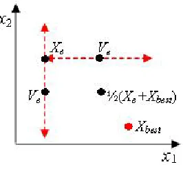
In the search Eq. (9) of ABC elite, (Xe,j +Xbest,j)/2 in the right-hand side can be

called base vector, and the second termφe,j(Xbest,j−Xk,j)in the right-hand side can be

called disturbance vector. The meaning of the Eq. (9) is that thejth element of candidate solutionVewill be produced by imposing the disturbanceφe,j(Xbest,j−Xk,j)on the base

vector(Xe,j+Xbest,j)/2. It is worth noting that only elite solutions in the onlooker bee

phase of ABC elite have a chance of producing candidate solutions, which will enhance the exploitation ability of ABC. In the Eq. (9), three kind of individuals are involved, i.e. the elite individualsXe, the global best individualXbest, and the ordinary individual

Xk. Because the fitness value ofXeandXbestis generally far better than the ordinary

individual Xk, the disturbance vectorφe,j(Xbest,j −Xk,j)is relatively large for base

vector(Xe,j+Xbest,j)/2.The relatively large disturbanceφe,j(Xbest,j−Xk,j)embodies

the exploration ability of ABC elite, and the excellent(Xe,j+Xbest,j)/2embodies the

exploitation ability of ABC elite, thus the balance between exploration and exploitation can be maintained. It can be seen from Fig.1, which is illustrated by literature [5], the candidate solutionVecan be only generated at the red axis, which is closer to the current

best solution whenφe,j(Xbest,j−Xk,j)is small, but is far away from the current best

solution whenXkis inferior andφe,j(Xbest,j−Xk,j)) is big.

Therefore, this design can result in the lack of exploitation ability, especially in the mid-late stage of evolution process because the demand of exploitation ability in EAs is not constant from the beginning to the ending. Generally speaking, for an EA, high exploration ability is required in the beginning to find more potential positions, while high exploitation ability is needed for convergence in the end. This conclusion can also be found in some other EAs, one of the most remarkable instance is the wPSO [25], in which linearly diminished weight is used so as to gradually increase the exploitation ability of PSO.

(8)

Because the randomly selected elite individualXe0 has better fitness value than

or-dinary individualXk in general and thus|Xbest,j−Xe0_,j| < |X_best,j −X_k,j|with a

high probability, if Xk is replaced with another randomly selected eliteXe0 in the Eq.

(9), the disturbance ofφe,j(Xbest,j−Xk,j)to the base vector(Xe,j+Xbest,j)/2will be

diminished, thus the exploitation ability of the Eq. (9) will be strengthened. Based on the above observation, a novel search equation used in the onlooker bee phase is proposed as follows:

Ve,j=

1

2(Xe,j+Xbest,j) +φe,j(Xbest,j−Xe0,j) (13)

WhereXe0 is a randomly selected elite solution,e0not equal toe; the rest of Eq. (13)

is same as that in Eq. (9).

Based on the above analysis, the Eq. (13) has a high exploitation ability than that of the Eq. (9) by imposing a small disturbanceφe,j(Xbest,j−Xk,j)on the base vector

(Xe,j +Xbest,j)/2. However, both the exploration ability and exploitation ability are

needed in EAs. If all bees produce new food sources using the Eq. (13), the algorithm can easily get trapped in the local optima when solving complex multi-modal problems. In other words, the Eq. (9) is insufficient in exploitation ability, while Eq. (13) is inadequate in exploration ability. To address this contradiction, we propose a new search mechanism in which the selective probabilityPo is introduced to balance the exploration of Eq. (9)

and the exploitation of Eq. (13). If the randomly generated number in [0,1] is less thanPo,

the Eq. (9) will be executed, otherwise the Eq. (13) will be executed. Because the demand of exploitation ability in EAs is gradually increased, the parameterPowill be diminished

linearly from 1 to 0. (see Lines 20 to 26 in Algorithm 1).

By combining Eq. (8) and (12) used in the employed bee phase, the Eq. (9) and (13) used in the onlooker bee phase and the selective probabilityPoused to select the Eq. (9)

and (13), an improved ABC elite, IABC elite for short, is proposed. The pseudo-code of IABC elite is given in Algorithm 1.

Compared with the original ABC elite, the IABC elite adds no additional computa-tion load, the whole structure of IABC elite is the same as ABC elite. The only difference between the two algorithms lies in their search equations. Therefore, the total complex-ity of the IABC elite is the same as that of the ABC elite. Now that the complexcomplex-ity of ABC elite isO(D∗SN)) [5], the complexity of IABC elite is alsoO(D∗SN)), which is also the same as original ABC [5].

The major difference between ABC elite and IABC elite is that ABC elite employ only one search equation Eqs. (8) and (9) in the employed bee phase and onlooker bee phase, respectively, while IABC elite adopts two different search equations in each phase. When the experimental results are analyzed, it is shown that the integration of search equations is a better option than the single search equation used in ABC elite because each search equation contributes the local search ability or global search ability, thus, the global-local search abilities are better balanced by using different search equations.

5. Experiments and Discussions

(9)

DFSABC elite. We selected these ABC variants for comparison because the search equa-tion of the basic ABC algorithm is improved in these recently developed methods. DFS-ABC elite is a composite algorithm consisting of the DFS-ABC elite and the depth-first frame-work, showing relatively good performance when compared with other state-of-the-art algorithms.

5.1. Benchmark Functions and Parameter Settings

To analyze and compare the performance and accuracy of the proposed algorithm IABC elite, a set of 22 benchmark functions with dimensionD= 30are used in the experiments. For instance,f1 −f6 andf8 are the continuous unimodal functions;f7 is a discontinuous step function; f9 is a noisy quartic function. f10 is the Rosenbrock function which is unimodal for D = 2 andD = 3, while it may have multiple optimal solutions when D >3.f11−f22are multi-modal functions, and the number of their local optimal points increases exponentially with the problem dimension. The search range, the global opti-mal value, the acceptant value of each function and their definitions can be found in the literature [5]. When the objective function value of the best solution obtained by an algo-rithm in a run is less than the acceptant value, the run is regarded as a successful one.The performance evaluation metrics are the same as those in the literature [5], which are de-scribed as follows: (1) The mean and standard deviation of the best objective function value are obtained by each algorithm, which are used to evaluate the quality or accuracy of the solutions obtained by different algorithms. The smaller the value of this metric is, the higher quality/accuracy the solution has; (2) The average FES (AVEN) is required to reach the acceptant value, which is employed to evaluate the convergence speed. The smaller the value of this metric is, the faster the convergence speed is. Note that AVEN will only be calculated for the successful runs. If an algorithm cannot find any solution whose objective function value is smaller than the acceptant value in all runs, AVEN will be denoted by NA; (3) The success rate (SR%) of the 25 independent runs is utilized to evaluate the robustness or reliability of different algorithms. The greater the value of this metric is, the better the robustness/reliability is.

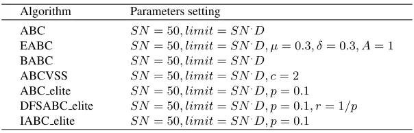
The parameter settings in the two experiments evaluated in the present paper have used the same settings of the ABC elite [5], and the maximal function evaluation (max F ES) is employed as the termination condition, which is set to 150000. For all the algorithms, SN is set to 50,D = 30,limit= SN.D; For the ABC-elite and DFSABC elite,pis set at 0.1. The parameter settings of all the other algorithms are set as suggested in their original papers shown in Table 1. All the algorithms are conducted with 25 independent runs for each test function.

In the two experiments evaluated in this paper, Experiment 1 is used to validate the effectiveness and efficiency of the improved algorithm (IABC elite). Experiment 2 is used to further evaluate the performance of IABC elite, when compared to other ABC variants developed recently.

(10)

Algorithm 1The procedure of IABC elite

1: Initialization:GenerateSNsolutions that contain variables according toEq.(1); 2: whileF es < max F esdo

3: Select the topT=p.SNsolutions as elite solutions from population; 4: fori= 1toSNdo

5: //employed bee phase 6: ifiis an elite solutionthen

7: Generate a new candidate solutionViin the neighborhood ofXiusingEq.(12);

8: else

9: Generate a new candidate solutionViin neighborhood ofXiusingEq.(8); 10: end if

11: Evaluate the new solutionVi; 12: iff(Vi)< f(Xi)then 13: ReplaceXibyVi; 14: counter(i)=0; 15: else

16: counter(i)= counter(i)+1; 17: end if

18: end for//end employed bee phase 19: fori= 1toSN do

20: //onlooker bee phase

21: Select a solutionXefrom elite solutions randomly to search; 22: Po= 1−F es/max F es;

23: ifrand(0,1)< Pothen

24: Generate a new candidate solutionVein neighborhood ofXeusingEq.(9); 25: else

26: Select a solutionXe0from elite solutions randomly, wheree0not equal toe;

27: Generate a new candidate solutionVeusingEq.(13); 28: end if

29: Evaluate the new solutionVe; 30: iff(Ve)< f(Xe)then 31: ReplaceXebyVe; 32: counter(e)=0; 33: else

34: counter(e)= counter(e)+1; 35: end if

36: end for//end onlooker bee phase 37: F es=F es+SN*2;

38: Select the solutionXmaxwith max counter value; //Scout bee phase 39: ifcounter(max)> limitthen

40: ReplaceXmaxby a new solution generated according toEq.(1); 41: F es=F es+ 1, counter(max) = 0;

(11)

Table 1.Parameters setting used in all experiments.

Algorithm Parameters setting ABC SN = 50, limit=SN._D

EABC SN = 50, limit=SN.D, µ= 0.3, δ= 0.3, A= 1

BABC SN = 50, limit=SN._D ABCVSS SN = 50, limit=SN.D, c= 2

ABC elite SN = 50, limit=SN._{D, p}_{= 0}_.₁

DFSABC elite SN = 50, limit=SN.D, p= 0.1, r= 1/p IABC elite SN = 50, limit=SN.D, p= 0.1

according to Wilcoxons rank test [6] at a 0.05 significance level. The last row in Table 2 and Table 3 each summarizes the comparison results.

5.2. Benchmark Functions and Parameter Settings

In this experiment, in order to validate the effectiveness and efficiency of IABC elite, the IABC-elite is compared with the ABC [13], BABC [8], ABC-elite [5] respectively. The results are shown in Table 2.

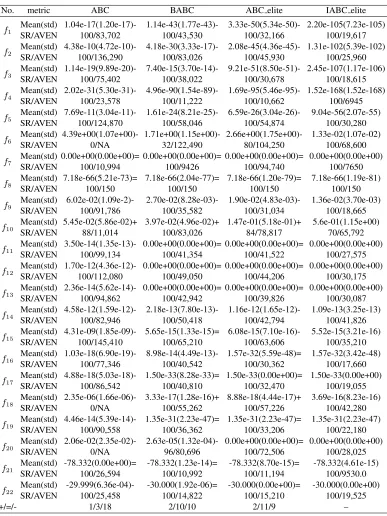
It can be clearly observed from Table 2 that the IABC elite outperforms all the other algorithms significantly in most of tested functions in terms of solution accuracy and convergence speed according to mean (std) and AVEN, respectively.

(1)T he comparative results of unimodal f unctions:f1−f9are unimodal func-tions. For functionsf1−f6, IABC elite demonstrates best performance in terms of so-lution accuracy and convergence speed according to mean(std) and AVEN, respectively. Because functionsf7andf8are easy to solve [5], the solution accuracy of all algorithms of this two functions are similar, but IABC elite has achieved better results regarding con-vergence speed. All in all, the results of IABC elite are better or at least similar to all other compared algorithms in all unimodal functions according to all test metrics.

The advantage of the IABC elite on unimodal is due to the novel Eq. (12) and Eq. (13), which can further enhance the exploitation ability of ABC elite.

(2)T he comparative results on multimodal f unctions: In multimodal functions f10−f22of Table 2, IABC elite also demonstrates good performance. Firstly, in the solu-tion accuracy, the IABC elite are better than or at least comparable to all other compared algorithms in all multimodal functions except for only 2 functions (f10andf18). Secondly, in the convergence speed AVEN, the IABC elite performs better than or at least compa-rable to all its competitors in all multimodal functions only except for the ABC elite on f22. Thirdly, in the metric SR, the IABC elite are better than or at least comparable to all other compared algorithms on all multimodal functions. The advantage of IABC elite on multimodal is due to the introduced parameterPo, which helps the IABC elite to maintain

a better balance between exploration and exploitation.

(12)

Table 2.The comparative results of ABC, BABC, ABC elite and IABC elite whenD=30.

No. metric ABC BABC ABC elite IABC elite

f1 Mean(std) 1.04e-17(1.20e-17)- 1.14e-43(1.77e-43)- 3.33e-50(5.34e-50)- 2.20e-105(7.23e-105)

SR/AVEN 100/83,702 100/43,530 100/32,166 100/19,617

SR/AVEN 100/136,290 100/83,026 100/45,930 100/25,960

SR/AVEN 100/75,402 100/38,022 100/30,678 100/18,615

SR/AVEN 100/23,578 100/11,222 100/10,662 100/6945

SR/AVEN 100/124,870 100/58,046 100/54,874 100/30,280

f6 Mean(std) 4.39e+00(1.07e+00)- 1.71e+00(1.15e+00)- 2.66e+00(1.75e+00)- 1.33e-02(1.07e-02)

SR/AVEN 0/NA 32/122,490 80/104,250 100/68,600

f7 Mean(std) 0.00e+00(0.00e+00)= 0.00e+00(0.00e+00)= 0.00e+00(0.00e+00)= 0.00e+00(0.00e+00)

SR/AVEN 100/10,994 100/9426 100/94,740 100/7650

f8 Mean(std) 7.18e-66(5.21e-73)= 7.18e-66(2.04e-77)= 7.18e-66(1.20e-79)= 7.18e-66(1.19e-81)

SR/AVEN 100/150 100/150 100/150 100/150

SR/AVEN 100/91,786 100/35,582 100/31,034 100/18,665

f10 Mean(std) 5.45e-02(5.86e-02)+ 3.97e-02(4.96e-02)+ 1.47e-01(5.18e-01)+ 5.6e-01(1.15e+00)

SR/AVEN 88/11,014 100/83,026 84/78,817 70/65,792

f11 Mean(std) 3.50e-14(1.35e-13)- 0.00e+00(0.00e+00)= 0.00e+00(0.00e+00)= 0.00e+00(0.00e+00)

SR/AVEN 100/99,134 100/41,354 100/41,522 100/27,575

SR/AVEN 100/112,080 100/49,050 100/44,206 100/30,175

SR/AVEN 100/94,862 100/42,942 100/39,826 100/30,087

SR/AVEN 100/82,946 100/50,418 100/42,794 100/41,826

f15 Mean(std) 4.31e-09(1.85e-09)- 5.65e-15(1.33e-15)= 6.08e-15(7.10e-16)- 5.52e-15(3.21e-16)

SR/AVEN 100/145,410 100/65,210 100/63,606 100/35,210

f16 Mean(std) 1.03e-18(6.90e-19)- 8.98e-14(4.49e-13)- 1.57e-32(5.59e-48)= 1.57e-32(3.42e-48)

SR/AVEN 100/77,346 100/40,542 100/30,362 100/17,660

f17 Mean(std) 4.88e-18(5.03e-18)- 1.50e-33(8.28e-33)= 1.50e-33(0.00e+00)= 1.50e-33(0.00e+00)

SR/AVEN 100/86,542 100/40,810 100/32,470 100/19,055

f18 Mean(std) 2.35e-06(1.66e-06)- 3.33e-17(1.28e-16)+ 8.88e-18(4.44e-17)+ 3.69e-16(8.23e-16)

SR/AVEN 0/NA 100/55,262 100/57,226 100/42,280

f19 Mean(std) 4.46e-14(5.39e-14)- 1.35e-31(2.23e-47)= 1.35e-31(2.23e-47)= 1.35e-31(2.23e-47)

SR/AVEN 100/90,558 100/36,362 100/33,206 100/22,180

f20 Mean(std) 2.06e-02(2.35e-02)- 2.63e-05(1.32e-04)- 0.00e+00(0.00e+00)= 0.00e+00(0.00e+00)

SR/AVEN 0/NA 96/80,696 100/72,506 100/28,025

f21 Mean(std) -78.332(0.00e+00)= -78.332(1.23e-14)= -78.332(8.70e-15)= -78.332(4.61e-15)

SR/AVEN 100/26,594 100/10,992 100/11,194 100/9530.0

f22 Mean(std) -29.999(6.36e-04)- -30.000(1.92e-06)= -30.000(0.00e+00)= -30.000(0.00e+00)

SR/AVEN 100/25,458 100/14,822 100/15,210 100/19,525

(13)

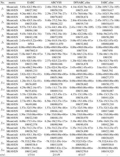
Table 3.The comparative results of EABC, ABCVSS, DFSABC elite and IABC elite whenD=30.

No. metric EABC ABCVSS DFSABC elite IABC elite

SR/AVEN 100/27,982 100/50,526 100/21,410 100/19,617

SR/AVEN 100/39,006 100/78,802 100/28,674 100/25,960

SR/AVEN 100/25,826 100/46,222 100/19,710 100/18,615

SR/AVEN 100/84,180 100/15,818 100/7122 100/6945

SR/AVEN 100/42,198 100/72,958 100/33,426 100/30,280

f6 Mean(std) 2.43e+01(5.22e+00)- 2.56e-01(9.19e-02)- 5.08e-07(3.69e-07)+ 1.33e-02(1.07e-02)

SR/AVEN 0/NA 100/111,070 100/32,802 100/68,600

f7 Mean(std) 0.00e+00(0.00e+00)= 0.00e+00(0.00e+00)= 0.00e+00(0.00e+0)= 0.00e+00(0.00e+00)

SR/AVEN 100/7602.0 100/10,042 100/7534 100/7450

f8 Mean(std) 7.18e-66/(7.49e-67)= 7.18e-66(9.98e-78)= 7.18e-66(3.23e-81)= 7.18e-66(1.19e-81)

SR/AVEN 100/150 100/150 100/150 100/150

f9 Mean(std) 1.65e-02(3.68e-03)- 2.57e-02(5.22e-03)- 1.20e-02(3.80e-03)+ 1.36e-02(3.70e-03)

SR/AVEN 100/23,398 100/40,846 100/16,878 100/18,665

f10 Mean(std) 1.14e+00(2.94e+00)- 3.25e-02(4.58e-02)+ 3.45e+00(1.45e+01)- 5.6e-01(1.15e+00)

SR/AVEN 100/85,233 96/86,483 60/58,683 70/65,792

SR/AVEN 96/34,067 100/51,966 100/27,754 100/27,575

SR/AVEN 88/36,005 100/60,578 100/28,602 100/30,175

f13 Mean(std) 4.29e-08(2.14e-07)- 3.45e-11(1.73e-10)- 0.00e+00(0.00e+00)= 0.00e+00(0.00e+00)

SR/AVEN 96/35,654) 100/69,514 100/31,066 100/30,087

SR/AVEN 100/38,454 100/52,906 100/34,430 100/41,826

f15 Mean(std) 2.73e-05(1.36e-04)- 6.50e-15(2.27e-15)= 3.80e-15(1.69e-15)+ 5.52e-15(3.21e-15)

SR/AVEN 96/49,888 100/80,074 100/37,998 100/35,210

SR/AVEN 100/24,862 100/46,142 100/18,902 100/17,660

f17 Mean(std) 1.50e-33(0.00e+00)= 1.50e-33(0.00e+00)= 1.50e-33(0.00e+00)= 1.50e-33(0.00e+00)

SR/AVEN 100/22,540 100/48,154 100/20,970 100/19,055

f18 Mean(std) 6.00e-17(3.41e-16)+ 6.26e-18(2.91e-17)+ 3.10e-40(1.03e-39)+ 3.69e-16(8.23e-16)

SR/AVEN 100/42,578 100/80,966 100/40,454 100/42,280

SR/AVEN 100/26,762 100/48,330 100/24,890 100/22,180

SR/AVEN 64/58,950 100/93,050 100/55,910 100/28,025

f21 Mean(std) -78.332(2.90e-15)= -78.332(1.05e-14)= -78.332(5.02e-15)= -78.332(4.61e-15)

SR/AVEN 100/8538.0 100/13,038 100/6502.0 100/9530.0

f22 Mean(std) -30.000(1.51e-06)= -30.000(3.82e-12)= -30.000(0.00e+00)= -30.000(0.00e+00)

SR/AVEN 100/12,602 100/18,726 100/5270.0 100/19,525

(14)

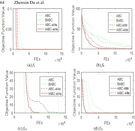
Fig. 2.The convergence curves of ABC, BABC, ABC elite and IABC elite on 4 repre-sentative test

5.3. Experiment 2: comparison of the IABC elite and other ABC variants

In this section, in order to further evaluate the performance of IABC elite, the IABC elite is compared with 3 recently developed representative ABC variants, i.e.,the EABC [12], ABCVSS [23], DFSABC elite [5] on all 22 test functions with 30D. The parameter set-tings are shown in Table 1, and the termination conditionmax F ESis the same as ex-periment 1 (max F ES = 150000). All the compared ABC variants have proposed an improved search equation. It’s worth noting that the DFSABC elite is a composite algo-rithm consisting of the ABC elite and depth-first strategy (DFS). The comparative results are shown in Table 3.

(1)T he comparative results on unimodal f unctions:

f1 −f9 are unimodal functions. For functions f1 −f5,According to Table 3, the IABC elite performs significantly better than all compared algorithms regarding solution accuracy (mean(std)) and convergence speed (AVEN), and all algorithms obtain the same results in the success rate (SR). For functionsf7−f8, although all the algorithms get the similar performance regarding solution accuracy and success rate becausef7−f8are easy to solve [5], the convergence speed of the IABC elite is faster than or at least com-parable to all the competitors. For functionsf6andf9, the IABC elite is only second to the DFSABC elite regarding solution accuracy and convergence speed, while IABC elite exhibits best success rate, beating all its competitors. In a word, the IABC elite shows the best overall performance in unimodal functions.

(15)

f10−f22are multimodal functions.f10is Rosenbrock function and its global optimum is inside a long, narrow, parabolic shaped flat valley, the variables are strongly dependent, and the gradients do not generally point towards the optimum. If the population is guided by the global best solution or some other good solutions, the search will fall into some un-promising areas. Therefore, DFSABC elite is beaten by all the competitors, even original ABC is also far better than DFSABC elite in functionf10.This phenomenon reflects the defect of DFS strategy used in DFSABC elite. Because the DFS strategy always search a direction greedily, it tends to result in lacking of randomness of EA and make it trapped into local optima. And the same conclusion can be drawn from literature [5] (see Table 3 of literature [5]). For functionf10, the IABC elite is better than the DFSABC elite and EABC, but still worse than ABCVSS slightly, regarding solution accuracy.

The last row of the Table 3 summarizes the comparison results. It can be seen that the IABC elite exhibits significantly advantage when compared with other algorithms. In the comparison with the DFSABC elite, IABC elite wins over it in 7 functions, ties in 11 functions while losed on 4 functions regarding solution accuracy. Although the DFS-ABC elite has combined with the DFS strategy, IDFS-ABC elite still outperform it. Similarly, the IABC elite performs better than the EABC and ABCVSS on most of the test functions regarding solution accuracy.

Overall, the IABC elite still performs better than all other algorithms on most of mul-timodal functions.

6. Conclusions

In order to increase the exploitation ability of the ABC elite and seek a better balance be-tween the abilities of exploration and exploitation, an improved ABC elite (the IABC elite) algorithm is put forward in this paper, combining two novel search equation and a new parameter with ABC elite. The first search equation is used in employed bee phase, thus the elite solutions and ordinary solutions adopt different search equation. The second search equation is used in the onlooker bee phase to further enhance the exploitation of the ABC elite. The new parameterPois introduced to maintain the balance between the

ability of exploration and that of exploitation. The experiment results have shown that the IABC elite can significantly improve the performance of ABC elite. When further compared to other state-of-the-art ABC variants, IABC elite also exhibits the best overall performance.

Acknowledgments.This work has been supported by the National Natural Science Foundation of China (No. 61373028 and No. 61672338).

References

1. B. Akay and D. Karaboga. A modified artificial bee colony algorithm for real-parameter opti-mization. Information Sciences, 192(12):120–142, 2012.

2. A. Banharnsakun, T. Achalakul, and B. Sirinaovakul. The best-so-far selection in artificial bee colony algorithm. Applied Soft Computing, 11(2):2888–2901, 2011.

(16)

4. D. Bose, S. Biswas, and A. V. Vasilakos. Optimal filter design using an improved artificial bee colony algorithm. Information Sciences, 281(20):443–461, 2014.

5. L. Cui, G. Li, and Q. Lin. A novel artificial bee colony algorithm with depth-first search framework and elite-guided search equation.Information Sciences, 367(22):1012–1044, 2016. 6. J. Derrac and S. Garca. A practical tutorial on the use of nonparametric statistical tests as a methodology for comparing evolutionary and swarm intelligence algorithms. volume 1 of1, pages 3–18. 2011.

7. R. Eberhart and J. Kennedy. A new optimizer using particle swarm theory. InMicro Machine and Human Science, 1995. MHS’95., pages 39–43. Proceedings of the Sixth International Sym-posium on.IEEE, 1995.

8. W. Gao, F. T. S. Chan, and L. Huang. Bare bones artificial bee colony algorithm with parameter adaptation and fitness-based neighborhood.Information Sciences, 316(18):180–200, 2015. 9. W. Gao and S. Liu. Improved artificial bee colony algorithm for global optimization.

Informa-tion Processing Letters, 111(17):871–882, 2011.

10. W. Gao and S. Liu. A modified artificial bee colony algorithm. Computers and Operations Research, 39(3):687–697, 2012.

11. W. Gao, S. Liu, and L. Huang. A novel artificial bee colony algorithm based on modified search equation and orthogonal learning.IEEE Transactions on Cybernetics, 43(3):1011–1024, 2013. 12. W. Gao, S. Liu, and L. Huang. Enhancing artificial bee colony algorithm using more

information-based search equations.Information Sciences, 270(12):112–133, 2014.

13. D. Karaboga. An idea based on honey bee swarm for numerical optimization, 2005. Ereiyes University.

14. D. Karaboga. A quick artificial bee colony (qabc) algorithm and its performance on optimiza-tion problems.Applied Soft Computing, 23(10):227–238, 2014.

15. J. Kennedy. Bare bones particle swarms.SIS’03. Proceedings of the 2003 IEEE. IEEE, (1):80– 87, 2003.

16. J. Kennedy. Particle swarm optimization. Encyclopedia of machine learning. Springer US, pages 760–766, 2011.

17. G. Li, P. Niu, and X. Xiao. Development and investigation of efficient artificial bee colony algorithm for numerical function optimization. Applied soft computing, 12(1):320–332, 2012. 18. W. H. Lim and N. A. M. Isa. Two-layer particle swarm optimization with intelligent division

of labor.Engineering Applications of Artificial Intelligence, 26(10):2327–2348, 2013. 19. W. H. Lim and N. A. M. Isa. An adaptive two-layer particle swarm optimization with elitist

learning strategy. Information Sciences, 273(14):49–72, 2014.

20. W. H. Lim and N. A. M. Isa. Adaptive division of labor particle swarm optimization. Expert Systems with Applications, 42(14):5887–5903, 2015.

21. J. Luo, Q. Wang, and X. Xiao. A modified artificial bee colony algorithm based on converge-onlookers approach for global optimization.Applied Mathematics and Computation, 219(20):10253–10262, 2013.

22. Q. K. Pan, L. Wang, and J. Q. Li. A novel discrete artificial bee colony algorithm forthe hybrid flowshop scheduling problem with makespan minimisation. 45(6):42–56, 2014.

23. Kiran M S, Hakli H, and Gunduz M. Artificial bee colony algorithm with variable search strategy for continuous optimization.Information Sciences, 300(8):140–157, 2015.

24. A. Salman, M. G. H. Omran, and M. Clerc. Improving the performance of comprehensive learning particle swarm optimizer. Journal of Intelligent and Fuzzy Systems, 30(2):735–746, 2016.

25. Y. Shi and R. Eberhart. A modified particle swarm optimizer. InEvolutionary Computa-tion Proceedings, pages 69–73. IEEE World Congress on Computational Intelligence.The 1998 IEEE International Conference on. IEEE, 1998.

(17)

27. H. Wang, Z. Wu, and S. Rahnamayan. Multi-strategy ensemble artificial bee colony algorithm. Information Sciences, 279(18):587–603, 2014.

28. G. Zhu and S. Kwong. Gbest-guided artificial bee colony algorithm for numerical function optimization. Applied Mathematics and Computation, 217(7):3166–3173, 2010.

Zhenxin Dureceived the B.S. degree in computer science from Zhejiang Sci-tech Univer-sity in 2011. He is currently a Ph.D. candidate at Shanghai Maritime UniverUniver-sity. His main research interests include computation intelligence, data mining and cloud computing.

Dezhi Han(corresponding author) received the Ph.D. degree from Huazhong University of Science and Technology. He is currently a professor of computer science and engi-neering at Shanghai Maritime University. His research interests include cloud computing, mobile networking and cloud security.

Guangzhong Liureceived the Ph.D. degree from China University of Mining and Tech-nology. He is currently a professor of computer science and engineering at Shanghai Mar-itime University. His specific research interests include underwater acoustic communica-tion technology, mobile networking and network security.

Kun Bireceived the Ph.D. degree from University of Science and Technology of China. He is currently a lecture of computer science and engineering at Shanghai Maritime Uni-versity. His research interests include network security, big data and cloud security.

Jianxin Jiareceived the M.S. degree from Shanghai Maritime University of computer science and engineering. He is currently pursuing the Ph.D. degree at Shanghai Maritime University. His main research interests include mobile networking, underwater acoustic communication technology and cloud security.

(18)