III
R
S
I
D
A
D
· C
A RL O S I II · DE
M
A
D
UNIVERSITY CARLOS III OF MADRID
Department of Telematics Engineering
Master of Science Thesis
A Control Theoretic Approach for Throughput Optimisation in
IEEE 802.11e EDCA WLANs
Author: Paul Horat»iu P˘atras»
Dipl.Eng. in Telecommunications
Supervisors: Albert Banchs Roca, Ph.D.
Pablo Serrano Y´a ˜nez-Mingot, Ph.D.
The MAC layer of the 802.11 standard, based on the CSMA/CA mechanism, specifies a set of parameters to control the aggressiveness of stations when trying to access the channel. However, these parameters are statically set independently of the conditions of the WLAN (e.g. the number of contending stations), leading to poor performance for most scenarios. To overcome this limitation previous work proposes to adapt the value of one of those parame-ters, namely the CW, based on an estimation of the conditions of the WLAN. However, these approaches suffer from two major drawbacks: i) they require extending the capabilities of standard devices orii) are based on heuristics.
This thesis proposes a control theoretic approach to adapt the CW to the conditions of the WLAN, based on an analytical model of its operation, that is fully compliant with the 802.11e standard. We use a Proportional Integrator controller in order to drive the WLAN to its optimal point of operation and perform a theoretic analysis to determine its configura-tion. We show by means of an exhaustive performance evaluation that our algorithm max-imises the total throughput of the WLAN and substantially outperforms previous standard-compliant proposals.
1 Introduction 1
2 State of the Art 3
2.1 IEEE 802.11e EDCA . . . 3
2.2 Distributed CW Adjustment Mechanisms . . . 5
2.2.1 Slow Decrease Algorithm . . . 5
2.2.2 CW Idle-Slots-based Control . . . 6
2.3 Centralised CW Adjustment Mechanisms . . . 7
2.3.1 Sliding Contention Window . . . 7
2.3.2 Dynamic Tuning Algorithm . . . 8
2.4 Optimal Configuration Prerequisites . . . 9
3 A Control Theoretic Approach for Throughput Optimisation 10 3.1 Throughput Analysis and Optimisation . . . 10
3.2 Adaptive Algorithm . . . 12
3.2.1 CW Configuration . . . 13
3.2.2 Control System . . . 13
4 Performance Evaluation 18 4.1 Throughput Performance . . . 18
4.2 Stability . . . 18
4.3 Speed of Reaction to Changes . . . 19
4.4 Non-saturated Stations . . . 22
4.5 Bursty Traffic . . . 23
4.6 Comparison Against Other Approaches . . . 23
4.7 Non-ideal Channel . . . 24
5 Summary 26
Appendix 27
References 28
2.1 Example of EDCA mechanism. . . 5
3.1 Control system. . . 14
3.2 Linearised system. . . 16
4.1 Throughput performance. . . 19
4.2 Stable configuration. . . 20
4.3 Unstable configuration. . . 20
4.4 Speed of reaction to changes. . . 21
4.5 Instantaneous throughput. . . 21
4.6 Non-saturated stations. . . 22
4.7 Bursty traffic. . . 23
4.8 Comparison against other approaches. . . 24
4.9 Capture effect. . . 25
Introduction
Wireless Local Area Networks (WLANs) have become a popular solution for provid-ing Internet connectivity anywhere and anytime due to their low cost and ease of deploy-ment. The IEEE 802.11 standard [18] defines two mechanisms for accessing the medium: a centralised one, named the point coordination function (PCF) and a distributed one, the distributed coordination function (DCF).
For the basic access mechanism, the standard defines a set of parameters that controls the way stations access the channel. Since radio channels have limited resources, they are shared by multiple users and multimedia applications need to be supported, optimising throughput and providing fair treatment to all stations require optimal configuration of the channel ac-cess parameters. In particular, the Contention Window (CW) parameter controls the prob-ability that a station defers or transmits a frame once the medium has become idle, and its value has a strong impact on the throughput of the WLAN.
The CW configuration used by the 802.11 standard [18] is statically set, independently of the number of contending stations. This static configuration leads to poor performance in most scenarios. In particular, when there are many stations in the WLAN it would be desirable to have larger CWs in order to avoid too frequent collisions, while with few sta-tions smaller CWs would help to reduce the channel idle time. Following this, it has been shown that for a given number of actively contending stations there exists an optimal CW configuration that maximises throughput performance [7, 4].
Following the above observations, many authors have proposed to dynamically adapt the CW by estimating the number of active stations in the WLAN. These works can be classified in two different groups:
1. Distributed approaches [8, 25, 22, 23, 24, 3, 14, 10, 9, 26], that require every node on the WLAN to implement a mechanism for adjusting the backoff behaviour. The main disadvantage of these approaches is that they change the rules of the 802.11 standard and require introducing modifications to the existing hardware.
2. Centralised approaches [21, 13], based on a single node that periodically distributes the set of MAC layer parameters to be used by every station. These approaches are compatible with the 802.11e standard. However, because they are based on heuristic algorithms and lack analytical support, they do not guarantee optimal performance.
In this thesis we propose a novel adaptive algorithm to dynamically adjust the CW configuration of 802.11-based Wireless LANs. We share the same goal with previous ap-proaches, i.e., to maximise the overall throughput performance of the wireless network. Compared to the existing schemes our proposal benefits from the following key improve-ments:
• It is fully compatible with the 802.11e standard and does not require any modifica-tion to existing hardware, since the dynamic adjustment is based only on observing successfully received frames at the Access Point (AP).
• It is based on a well established scheme from discrete-time control theory, namely the Proportional Integrator (PI). We optimally tune the parameters of the PI controller by conducting a control theoretic analysis of the system.
State of the Art
In this chapter we first present the EDCA mechanism of IEEE 802.11a which supports service differentiation as well as reconfiguration of the MAC parameters. Next we sum-marise the principles of several previous proposals that aim to adjust the MAC parameters of the WLANs with the goal of optimising the throughput. Nevertheless, we list a set of rules that have been taken into account when designing our CW control algorithm.
2.1
IEEE 802.11e EDCA
This section briefly summarises the EDCA mechanism. This mechanism has been de-fined in the 802.11e standard [19] and will be included in the ongoing new revision of the 802.11 standard [20].
DCF is the fundamental channel access scheme in IEEE 802.11 WLANs, based on the carrier sense multiple access with collision avoidance (CSMA/CA) mechanism [7]. Two ways of accessing the channel are defined. The default mechanism assumes a 2-way hand-shake, i.e. after each transmission an acknowledgement frame is sent to confirm the correct reception of the frame (basic access mechanism). The second method is optional and re-quires a 4-way handshaking procedure, known as RTS/CTS. A station will try to reserve the channel prior to a transmission by sending a request-to-send frame (RTS). The receiving station will reply with a clear-to-send (CTS) frame if no collision was involved and the basic transmission-acknowledge mechanism will begin. This aims to minimize the time a station spends resolving collisions but also to avoid the hidden-terminal problem [11].
EDCA (Enhanced Distributed Channel Access) regulates the access to the wireless chan-nel on the basis of the chanchan-nel access functions (CAFs). A station may run up to 4 CAFs, and each of the frames generated by the station is mapped to one of them. Once a station becomes active, each CAF executes an independent backoff process to transmit its frames.
A station with a new frame to transmit monitors the channel activity. If the medium is idle for a period of time equal to the arbitration interframe space parameter (AIF S), the CAF transmits. Otherwise, if the channel is sensed busy (either immediately or during the
AIF S period), the CAF continues to monitor the channel until it is measured idle for an
AIF Stime, and, at this point, the backoff process starts.
Upon starting the backoff process, a random value uniformly distributed in the range
(0, CW−1)is chosen and the backoff time counter is initialized with this number. TheCW
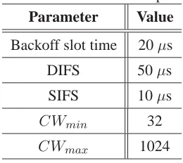
Table 2.1: IEEE 802.11b MAC parameters
Parameter Value
Backoff slot time 20μs
DIFS 50μs
SIFS 10μs
CWmin 32
CWmax 1024
value is called the contention window, and depends on the number of failed transmissions of a frame. At the first transmission attempt,CW is set equal to the minimum contention window parameter (CWmin).
As long as the channel is sensed idle, the backoff time counter is decremented once every empty slot time Te. When a transmission is detected on the channel, the backoff
time counter is “frozen”, and reactivated again after the channel is sensed idle for a certain period. This period is equal to AIF S if the transmission is received with a correct FCS, andEIF S−DIF S+AIF Sotherwise, whereEIF S (the extended interframe space) and
DIF S (the distributed interframe space) are physical layer constants.
As soon as the backoff time counter reaches zero, the CAF transmits its frame. A colli-sion occurs when two or more CAFs start transmitting simultaneously. An acknowledgement (Ack) frame is used to notify the transmitting station that the frame has been successfully received. The Ack is sent upon the reception of the frame, after a period of time equal to the physical layer constant SIFS (the short interframe space).
If the Ack is not received within a time interval given by the Ack T imeout physical layer constant, the CAF assumes that the frame was not received successfully. The transmis-sion is then rescheduled by re-entering the backoff process, which starts at anAIF S time following the timeout expiry. After each unsuccessful transmission,CW is doubled, up to a maximum value given by theCWmaxparameter. If the number of failed attempts reaches
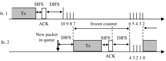
a predetermined retry limitR, the frame is discarded. This mechanism is illustrated in Fig. 2.1 for a simple scenario with two active stations using a minimum AIFS parameter (equal to DIFS) and the default IEEE 802.11b MAC parameters. The values of these parameters are listed in Table 2.1.
After a (successful or unsuccessful) frame transmission, before sending the next frame, the CAF must execute a new backoff process. As an exception to this rule, the protocol allows the continuation of an EDCA transmission opportunity (TXOP). A continuation of an EDCA TXOP occurs when a CAF retains the right to access the channel following the completion of a transmission. In this situation, the station is allowed to send a new frame a SIFS period after the completion of the previous one. The period of time a CAF is allowed to retain the right to access the channel is limited by the transmission opportunity limit parameter (T XOP limit).
St. 1
St. 2 Tx
SIFS
ACK DIFS
New packet
in queue DIFS
Tx
10 9 8 7 frozen counter 6 5 4 3 2
DIFS SIFS
ACK 4 3 2 1 0
Figure 2.1: Example of EDCA mechanism.
priority CAF. The other CAFs of the station involved in the internal collision react as if there had been a collision on the channel, doubling theirCW and restarting the backoff process.
As it can be seen from the description of EDCA given in this section, the behaviour of a CAF depends on a number of parameters, namely CWmin, CWmax, AIF S and
T XOP limit. These are configurable parameters that can be set to different values for different CAFs. The CAFs are grouped by Access Categories (ACs), all the CAFs of an AC having the same configuration. The Access Point (AP) announces periodically (every 100 ms) the parameters of each AC by means of beacon frames.
Following the above considerations several adaptive algorithms have been proposed trying to adjust the value of the contention window, such that throughput optimisation is achieved. The works published until now are mainly focusing on two approaches. One consists of observing the channel state and modifying theCW at every station (distributed method), e.g. [8, 25, 22, 23, 24, 3, 14, 10, 9, 26] and the second assumes monitoring the contention level at the access point, tuning theCW appropriately and distributing it to the as-sociated stations (centralised method), e.g. [13, 21]. With the approval of the IEEE 802.11e standard [19], changing of the CW value is now allowed to be performed by means of beacon frames with an adjustment granularity equal to the beacon interval (100ms).
2.2
Distributed CW Adjustment Mechanisms
The other approach to adaptiveCW control involves monitoring of the network state at every station and independently adjusting the configuration of the EDCA parameters. The advantages of such techniques are the following:
• They do not require estimation of the number of station actively contending for the channel
• Each station’s adjustment mechanism is independent from the one employed by other stations.
2.2.1 Slow Decrease Algorithm
[22] considers that a successful transmission doesn’t reflect a congestion level decrease, but rather a convenient CW value. Therefore, theCW value should be maintained as long as the congestion level remains the same. The second assumption made by this proposal is that the congestion level is not likely to decrease sharply. Hence, by resettingCW toCWminthe
risk of experiencing collisions and retransmissions until reaching a high value again is large. This also leads to channel underutilisation. The slow decrease (SD) algorithm attempts to minimize the number of collisions during congestion, but, by keeping the sameCW values when congestion sharply drops, increases the overhead and may decrease the throughput. The slow decrease factorδis in the range (0,1). The behaviour of the SD algorithm is shown below.
Algorithm 1 Slow Decrease Algorithm 1: ifT x successf ulthen
2: CWnew←max(CWmin, δ·CWold)
3: else
4: CWnew←min(2·CWold, CWmax)
5: end if
2.2.2 CW Idle-Slots-based Control
Another distributed CW adjustment scheme was proposed by Xia et al. in [25]. The
CW Idle-Slots-based Control (WISC) is significantly different from the standard BEB mechanism. The adjustment scheme is based on a control-theoretic approach that dynami-cally adjusts theCW based on the locally available channel state. The average number of consecutive idle slots between two transmissions is monitored and then used to drive the
CW to its optimal value, such that throughput is maximised. This mechanism is extremely accurate but requires large processing overhead, since theCW is adjusted after each trans-mitted frame.
Algorithm 2 CW Idle-Slots-based Control Algorithm
1: while Tx attempt do
2: eprev←ecur
3: ecur←Im−I(t)
4: CWcur←CWcur+C1·ecur+C2·eprev
5: ifCWcur< CWminthen
6: CWcur ←CWmin
7: end if
8: ifCWcur> CWmaxthen
9: CWcur ←CWmax
10: end if
11: end while
also holds the optimalCW value. Hence, by tuning theCW such that the number of idle slotsI(t)is around the optimalIm value, the throughput of the network will be optimized.
The optimal value of idle-slots between two transmissions has been previously estimated by [15] to be Im ≈ 5.68. The formal description of WISC is illustrated in Algorithm 2.
The values of theC1 andC2 coefficients have been derived using analytical methods form control theory and are 11.75 and 5.75 respectively.
Although outperforming the default DCF mechanism, distributed solutions suffer from some significant drawbacks in terms of their practical use. First of all, they require modifica-tions of the station’s hardware and drivers since the backoff rules are embedded inside them. Moreover, each station requires additional CPU time for running the algorithm locally and additional transmission delay is introduced. In what follows we will present a set of different approaches that try to overcome these limitations by adjusting the WLAN parameters in a single node and distributing them to the other stations.
2.3
Centralised CW Adjustment Mechanisms
In the IEEE 802.11e standard [19] it is specified that the WLAN configuration can be changed by the AP using beacons. The values ofCWmin andCWmax can be distributed
to all the stations every beacon interval. Several algorithms making use of this feature have been proposed to dynamically adjust the value of theCW such that throughput is optimized. In what follows we will present the mechanisms employed by two such solutions, namely the Sliding Contention Window (SCW) [21] and the algorithm presented in [13], hereafter referred to as Dynamic Tuning Algorithm (DTA). The advantages of these approaches are the following:
• They do not require any modification of the hardware or drivers on the stations
• They react to changes in the network load
2.3.1 Sliding Contention Window
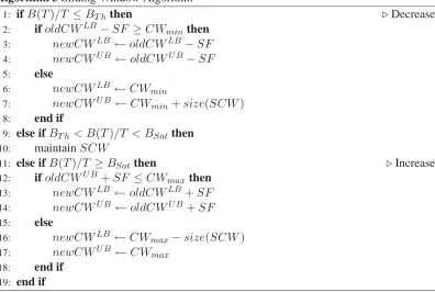
SCW was designed to maximise network utilisation and provide traffic differentiation by modifying the ranges from which the backoff counter is chosen. The sliding contention window of each traffic class has a lower boundCWLB and an upper boundCWU B. These bounds change but remain within the interval(CWmin, CWmax). To adjust theCW range,
SCW uses a linear-increase linear-decrease model, increasing or decreasing the SCW range in steps of a sliding factor SF. When a flow experiences high loss rate, the SCW is increased by a step of SF until it reaches the upper bound, while if the loss rate is low, instead of resetting the contention window value, the range is decreased until the lower bound reaches
CWmin. The adjustment of theCW range for best effort traffic is based on the observation
of the instantaneous network load B(T). B(T) is the fraction of slots the medium was detected busy out of the previousT slots. If the network load drops below a thresholdBT h,
the SCW range is decreased, while if it exceeds the throughput saturation thresholdBSatthe
range will be increased. The authors have chosen by means of simulation the values forBT h
Algorithm 3 Sliding Window Algorithm
1: ifB(T)/T ≤BT hthen Decrease
2: ifoldCWLB−SF ≥CWminthen 3: newCWLB ←oldCWLB−SF 4: newCWU B ←oldCWU B−SF
5: else
6: newCWLB ←CWmin
7: newCWU B ←CWmin+size(SCW)
8: end if
9: else ifBT h< B(T)/T < BSatthen
10: maintainSCW
11: else ifB(T)/T ≥BSatthen Increase
12: ifoldCWU B+SF ≤CW
maxthen 13: newCWLB ←oldCWLB+SF 14: newCWU B ←oldCWU B+SF
15: else
16: newCWLB ←CWmax−size(SCW) 17: newCWU B ←CWmax
18: end if
19: end if
Table 2.2: Parameters of the SCW algorithm
Parameter Value (time slots)
SCWsize 256
SF 128
CWmin 128
CWmax 1024
The parameters used by the authors for adjusting theCW range under best effort traffic conditions are shown in Table 2.2.
2.3.2 Dynamic Tuning Algorithm
J. Freitag et al. proposed a different centralised algorithm that is based on estimating the number of stations served by an AP [13]. Their assumption is that when there are only few stations, a lowCWminwill reduce the station idle time and increase the channel utilization.
Also, when the number of stations is high,CWminshould be increased to avoid collisions.
The number of active stations may be determined by the AP by estimating the number of active flows and identifying their source address. Following this reasoning the dynamic tuning algorithm (DTA) will double the value ofCWmin if the number of active stations is
larger than CWmin. Otherwise, ifCWmin/2 is greater than the number of stations, it will
CWminandCWmin/2. Moreover, the algorithm checks whether the values ofCWmin are
below a minimum value. In this case, they will be set to the minimum value allowed. The AP will inform the stations of the new value ofCWminusing beacons.
Algorithm 4 Dynamic Tuning Algorithm 1: ifnum stations > CWminthen 2: CWmin←CWmin·2 + 1
3: end if
4: ifnum stations < CWmin/2then
5: CWmin←(CWmin−1)/2
6: end if
7: ifCWmin < CW M inimumthen 8: CWmin←CW M inimum
9: end if
2.4
Optimal Configuration Prerequisites
Our goal is to find the EDCA parameters that maximise the throughput of the WLAN, while fairly sharing the bandwidth among the competing stations. Following this goal, we use the following configuration for the stations:
• In an optimally configured WLAN collisions are very infrequent. Hence, the impact of avoiding some of them due to multiple CAFs is negligible. Consequently, we will assume each station executes a single CAF and transmits one frame upon accessing the channel.
• As proved in [6], if using an AIF S parameter different from the minimum value (DIF S), there exists at least another configuration with minimumAIF S that pro-vides equal or better throughput performance. Consequenty, we set theAIF S param-eter to the minimum value (DIF S) for all stations.
• All stations will contend with the sameCWmin andCWmax parameters in order to
guarantee equal probability of accessing the channel and same throughput guarantees.
In what follows we design an adaptive algorithm that adjusts the configuration ofCWmin
andCWmax with the goal of maximising the overall WLAN throughput. This algorithm
is executed at the AP, which uses beacon frames to announce the computed CWmin and
A Control Theoretic Approach for
Throughput Optimisation
In this chapter we conduct a mathematical analysis of the WLAN throughput and then we derive the conditions for which this is maximised. Then we present the principles of our CW configuration algorithm and analyse our control system from a theoretical viewpoint. Finally, we show how we configure our controller to achieve a proper trade-off between stability and speed of reaction to changes.
3.1
Throughput Analysis and Optimisation
In this chapter we present a throughput analysis of an EDCA WLAN configured accord-ing to the rules listed in section 2.4. Based on this analysis, we find the collision probability of an optimally configured WLAN, which is the basis of the algorithm presented in the following section.
We start by analysing the case when all stations are saturated1 and consider later the case when some stations are not saturated. Let us defineτ as the probability that a saturated station transmits at a randomly chosen slot time. This can be computed according to [7] as follows:
τ = 2
1 +W +pWmi=0−1(2p)i (3.1)
whereW =CWmin,mis the maximum backoff stage (CWmax= 2mCWmin) andpis the
probability that a transmission collides. In a WLAN withnstations,
p= 1−(1−τ)n−1 (3.2)
The throughput obtained by a station can be computed as follows
r= Psl
PsTs+PcTc+PeTe
(3.3)
wherelis the packet length,Ps,Pc andPeare the probabilities of a success, a collision and
an empty slot time, respectively, andTs,TcandTeare the respective slot time durations. 1
Following [7], by saturation we mean that a station always has a packet ready for transmission.
The probabilities Ps,PcandPeare computed as
Ps=nτ(1−τ)n−1 (3.4)
Pe= (1−τ)n (3.5)
Pc = 1−nτ(1−τ)n−1−(1−τ)n (3.6)
and the slot time durationsTsandTc as
Ts=TP LCP+HC +Cl +SIF S+TP LCP +AckC +DIF S (3.7)
Tc =TP LCP +H
C + l
C +DIF S (3.8)
where TP LCP is the PLCP (Physical Layer Convergence Protocol) preamble and header
transmission time, H is the MAC overhead (header and FCS), Ack is the size of the ac-knowledgement frame andCis the channel bit rate.
The above terminates our throughput analysis. We next address, based on this analysis, the issue of optimizing the throughput performance of the WLAN. To this aim, we can rearrange Eq. (3.3) to obtain
r= l
Ts−Tc+Pe(Te−PTsc)+Tc
(3.9)
As l, Ts, and Tc are constants, maximizing the following expression will result in the
maximization ofr,
ˆ
r = Ps Pe(Te−Tc) +Tc
(3.10)
Givenτ 1,rˆcan be approximated by
ˆ
r= nτ−n(n−1)τ
2
Te−n(Te−T c)τ +n(n2−1)(Te−Tc)τ2
(3.11)
The optimal value ofτ,τopt, that maximizesˆrcan then be obtained by
dˆr d τ
τ=τopt
= 0 (3.12)
which neglecting the terms of higher order than 2 yields
aτ2+bτ+c= 0 (3.13)
where
a=−n
2(n−1)
2 (Tc −Te) (3.14)
b=−2n(n−1)Te (3.15)
Isolatingτoptfrom the above yields
τopt =
2Te
n(Tc−Te)
2
+ 2Te
n(n−1)(Tc−Te) − 2Te
n(Tc−Te)
(3.17)
GivenTe Tc, we finally obtain the following approximate solution for the optimalτ,
τopt≈ n1
2Te
Tc
(3.18)
With the aboveτopt, the corresponding optimal collision probability is equal to
popt= 1−(1−τopt)n−1= 1−
1− 1
n
2Te
Tc n−1
(3.19)
which can be approximated by
popt≈1−e−
2Te
Tc (3.20)
This implies that, under optimal operation with saturated stations, the collision probabil-ity in the WLAN is a constant independent of the number of stations. The key approximation of this paper is to assume that, when some of the stations are saturated and some are not, the optimal collision of the WLAN takes the same constant value.
In the following section we design an adaptive algorithm that adjusts the WLAN con-figuration with the goal of driving the collision probability to the above value. Note that, since this a constant value, our algorithm does not need to know the number of stations in the WLAN.
3.2
Adaptive Algorithm
We next present our adaptive algorithm; this algorithm runs at the AP and consists of the following two steps which are executed iteratively:
• During the period between two beacon frames (which lasts 100 ms), the AP measures the collision probability of the WLAN resulting from the current CW configuration.
• At the end of this period, the AP computes the new CW configuration based on the measured collision probability and distributes it to the stations in a new beacon frame.
3.2.1 CW Configuration
Following the previous section, our goal is to adjust the CW parameters of EDCA (CWminandCWmax) in order to force the collision probability given by Eq. (3.20). Since
the defaultCW values given by the 802.11e standard2(CWmindef aultandCWmaxdef ault) are
typ-ically too small, yielding a too aggressive behaviour, in order to achieve optimal operation theseCW parameters should be increased.
Following the above reasoning, our algorithm increases the defaultCWminof the
stan-dard by someCWof f set,
CWmin =CWmindef ault+CWof f set (3.21)
while keeping the default value for the maximum backoff stage, i.e.
CWmax= 2mCWmin (3.22)
wheremis the maximum backoff stage of the default configuration.
In order to ensure that our algorithm never underperforms the standard default configura-tion by using overly smallCW values, we force thatCWof f setcannot take negative values,
which guarantees thatCWminwill never take smaller values than the standard’s default. In
addition, we also force thatCWof f set cannot take values that yield aCWmin larger than
CWmaxdef ault. These bounds provide a safeguard against too large and too small values of
CWmin, respectively. In the rest of the paper we assume thatCWof f setalways takes values
within these bounds and do not further consider this effect.
3.2.2 Control System
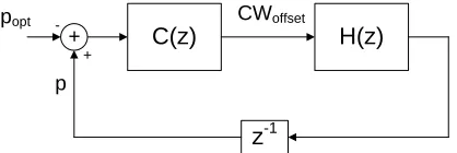
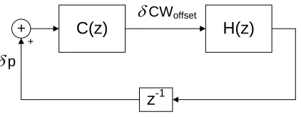
From a control theoretic standpoint, our system can be seen as the composition of the two modules depicted in Figure 3.1: the controller C(z), which is the adaptive algorithm that controls the WLAN, and the controlled system H(z), which is the WLAN itself. In our proposal we use for the controller module a classical scheme from discrete-time control theory, namely the Proportional Integrator (PI) Controller.
Following the above, our control system consists of the following two modules:
• The controller module located at the AP, that is based on the Proportional Integrator (PI) controller. The AP estimates the collision probability and provides it to the con-troller, which takes as input the difference between the estimated collision probability and its desired value as given by Eq. (3.20). With this input, the controller computes theCWof f setvalue.
• The controlled module is the 802.11e EDCA WLAN system. As specified by the stan-dard, the AP distributes the newCW configuration to the stations every 100 ms. This configuration is obtained from theCWof f setvalue given by the controller, following
Eqs. (3.21) and (3.22).
2
C(z) H(z)
z-1
+
-+
popt
p
CWoffset
Figure 3.1: Control system.
The estimation of the collision probability over a 100 ms period is performed at the AP as follows. LetS be the number of frames received by the AP during this period with the retry bit unset, andR be the number of frames received with the retry bit set. Then, if we assume that no frames are discarded due to reaching the retry limit, the collision probability
pcan be computed as
p= R
R+S (3.23)
since the above is precisely the probability that the first transmission attempt of a frame collides.
Note that with the above method, the AP can compute the probability p by simply analysing the header of the frames successfully received, which can be easily done with no modifications to the AP’s hardware and driver.
Transfer Function Characterisation
In order to analyse our system from a control theoretic standpoint, we need to charac-terise the Wireless LAN system with a transfer function that takes CWof f set as input and
gives the collision probabilitypas output. Since the collision probability is measured every 100 ms interval, we can safely assume that the obtained measurement corresponds to station-ary conditions and therefore the system does not have any memory. With this assumption,
p= 1−(1−τ)n−1 (3.24)
whereτ is a function ofCWof f set as given by Eq. (3.1),
τ = 2
1 + (CWdef ault
min +CWof f set)(1 +p
m−1
i=0 (2p)i)
(3.25)
The above equations give a nonlinear relationship betweenpandCWof f set. In order to
express this relationship as a transfer function, we linearise this relationship when the system is perturbed around its stable point of operation3, i.e.
CWof f set =CWof f set,opt+δCWof f set (3.26)
whereCWof f set,optis theCWof f setvalue that yields the optimal collision probabilitypopt
computed in Eq. (3.20).
With the above, the oscillations of the collision probability around its point of operation
poptcan be approximated by
p≈popt+∂CW∂p
of f setδCWof f set
(3.27)
The above partial derivative can be computed as
∂p ∂CWof f set =
∂p ∂τ
∂τ ∂CWof f set
(3.28)
where
∂p
∂τ ≈n−1 (3.29)
and
∂τ
∂CWof f set =−
2(1 +pmi=0−1(2p)i)
1 +CWmin(1 +p
m−1
i=0 (2p)i)
2 (3.30)
Evaluating the partial derivative at the stable point of operation p=popt, and using the
approximation popt ≈(n−1)τoptgiven by Eq. (3.19) and the expression forτoptgiven by
Eq. (3.1), yields
∂p
∂CWof f set ≈ −poptτopt
1 +popt
m−1
i=0 (2popt)i
2 (3.31)
If we now consider the transfer function that allows us to characterize the perturbations ofparound its stable point of operation as a function of the perturbations inCWof f set,
δP(z) =H(z)δCWof f set(z) (3.32)
we obtain from Eqs. (3.27) and (3.31) the following expression for the transfer function,
H(z) =−poptτopt1 +popt
m−1
i=0 (2popt)i
2 (3.33)
Figure 3.2 illustrates the above linearised model when working around its stable
opera-tion point:
p=popt+δp
CWof f set=CWof f set,opt+δCWof f set
(3.34)
Note that, as compared to the model of Figure 3.1, in Figure 3.2 only the perturbations around the stable operation point are considered.
Controller Configuration
We next address the issue of configuring the PI controller. The transfer function of the controller is given by
C(z) =Kp+ Ki
C(z) H(z)
z-1 +
+
p
CWoffset
G
G
Figure 3.2: Linearised system.
We observe from the above transfer function that the PI controller depends on the fol-lowing two parameters to be configured: KpandKi. Our goal in the configuration of these
parameters is to find the right trade-off between speed of reaction to changes and stability. To this aim, we use the Ziegler-Nichols rules [12] which have been designed for this purpose. These rules are applied as follows. First, we compute the parameterKu, defined as theKp
value that leads to instability whenKi = 0, and the parameterTi, defined as the oscillation
period under these conditions. Then,KpandKiare configured as follows:
Kp = 0.4Ku (3.36)
and
Ki= 0Kp
.85Ti
(3.37)
In order to compute Ku we proceed as follows. The system is stable as long as the
absolute value of the closed-loop gain is smaller than 1,
|H(z)C(z)|=Kppoptτopt1 +popt
m−1
i=0 (2popt)i
2 <1 (3.38)
which yields the following upper bound forKp,
Kp < 2
poptτopt(1 +poptim=0−1(2popt)i)
(3.39)
Since the above is a function ofn(note thatτoptdepends onn) and we want to find an
upper bound that is independent ofn, we proceed as follows. From Eq. (3.19), we observe thatτoptis never larger thanpoptforn >1(note that forn= 1the system is stable for any
Kp). With this observation, we obtain the following constant upper bound (independent of
n):
Kp < 2
p2opt(1 +popt
m−1
i=0 (2popt)i)
(3.40)
Following the above, we takeKuas the value where the system may turn unstable (given
by the previous equation),
Ku = 2
p2opt(1 +popt
m−1
i=0 (2popt)i)
and setKpaccording to Eq. (3.36),
Kp = 0.4·2
p2opt(1 +popt
m−1
i=0 (2popt)i)
(3.42)
With the Kp value that makes the system become unstable we haveH(z)C(z) = −1.
With such a closed-loop transfer function, a given input value changes its sign at every time slot, yielding an oscillation period of two slots (Ti= 2). Thus, from Eq. (3.37),
Ki = 0.4 0.85p2opt(1 +popt
m−1
i=0 (2popt)i)
(3.43)
Performance Evaluation
In order to evaluate the performance of the proposed algorithm, we performed an ex-haustive set of simulation experiments. For this purpose, we have extended the simulator used in [6, 5]; this is an event-driven simulator that closely follows the details of the MAC protocol of 802.11 EDCA. For all tests, we used a payload size of 1000 bytes and the sys-tem parameters of the IEEE 802.11b physical layer [17]. For the simulation results, average and 95% confidence interval values are given (note that in many cases confidence intervals are too small to be appreciated in the graphs). Unless otherwise stated, we assume that all stations are saturated.
4.1
Throughput Performance
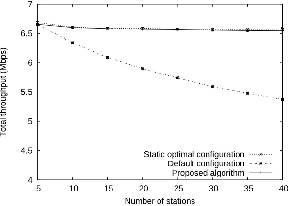
The main objective of the proposed algorithm is to maximize the throughput perfor-mance of the WLAN. To verify if the proposed algorithm meets this objective, we evaluated the total throughput obtained for different numbers of stations n. As a benchmark against which to assess the performance of our approach, we compared it against the static optimal configuration given by Eq. (3.18) and the default configuration given in the 802.11e stan-dard [19]. Note that the static optimal configuration method requires the knowledge of the number of active stations, which challenges its practical use.
The results of the experiment described above are given in Figure 4.1. We can observe from the figure that the performance of the proposed algorithm follows very closely the static optimal configuration in terms of total throughput. In contrast, the default configuration performs well for a small number of stations but sees its performance substantially degraded as the number of stations increases. From these results, we conclude that the proposed algorithm maximises the throughput performance.
4.2
Stability
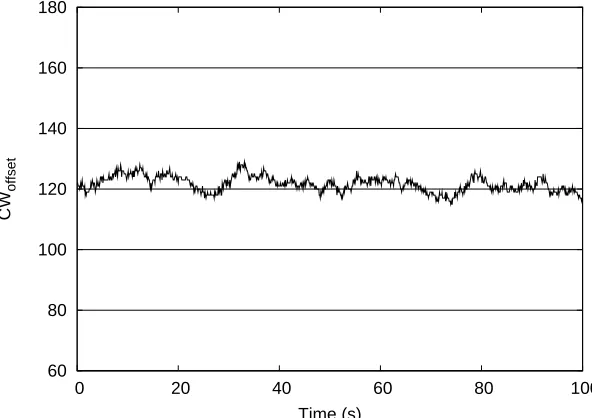
One of the objectives of the configuration of the PI controller presented in Section 3.2.2 is guaranteeing a stable behaviour of the system. In order to assess this objective, we plot in Figure 4.2 the value of the system’s control signal (CWof f set) every beacon interval, for
our{Kp, Ki}setting withn= 20stations. We can observe that with the proposed setting,
4 4.5 5 5.5 6 6.5 7
5 10 15 20 25 30 35 40
Total throughput (Mbps)
Number of stations
Static optimal configuration Default configuration Proposed algorithm
Figure 4.1: Throughput performance.
CWof f setperforms stably with minor deviations around its point of operation. In case that a
larger setting for{Kp, Ki}was used to improve the speed of reaction to changes, we would
have the situation of Figure 4.3. For this case, with values for{Kp, Ki}20 times larger, the
CWof f setshows a strong unstable behaviour with drastic oscillations. We conclude that the
proposed configuration achieves the objective of guaranteeing a stable behaviour.
4.3
Speed of Reaction to Changes
In addition to a stable behaviour, we also require the PI controller to quickly react to changes on the WLAN. To assess this objective we ran the following experiment. For a WLAN with 15 saturated stations, att = 80we added 15 more stations. We plot the be-haviour ofCWof f set for our{Kp, Ki}setting in Figure 4.4 (label “Kp, Ki”). The system
reacts fast to the changes on the WLAN, asCWof f setreaches the new value almost
imme-diately. We have already shown in the previous section that large values for the parameters of the controller lead to unstable behavior. To analyze the impact of small values for these parameters, we plot on the same figure theCWof f set evolution for a{Kp, Ki}setting 20
times smaller (label “Kp/20, Ki/20”). With such setting, although obtaining a minor gain in stability, the system reacts too slow to changes of the conditions on the WLAN.
60 80 100 120 140 160 180
0 20 40 60 80 100
CW
offset
Time (s)
Figure 4.2: Stable configuration.
60 80 100 120 140 160 180
0 20 40 60 80 100
CW
offset
Time (s)
0 50 100 150 200 250
0 100 200 300 400 500
CW
offset
Time (s)
Kp,Ki Kp/20,Ki/20
Figure 4.4: Speed of reaction to changes.
0 0.2 0.4 0.6 0.8 1
40 60 80 100 120
Instantaneous throughput (Mbps)
Time (s)
4 4.5 5 5.5 6 6.5 7
0 5 10 15 20 25 30 35 40
Total throughput (Mbps)
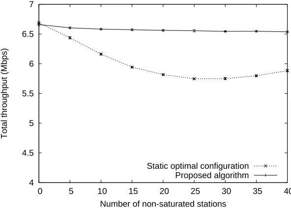
Number of non-saturated stations Static optimal configuration
Proposed algorithm
Figure 4.6: Non-saturated stations.
4.4
Non-saturated Stations
Our approach has been designed to optimise performance both under saturation and non-saturation conditions, in contrast to the static optimal configuration shown previously which is based on the assumption that all stations are saturated. In order to evaluate and compare the performance of the two algorithms when there are non-saturated stations in addition to saturated stations, we performed the following experiment. We had 5 saturated stations and a variable number of non-saturated stations in the WLAN. The non-saturated stations gener-ated CBR traffic at rate of 100 Kbps. The total throughput resulting from this experiment is illustrated in Figure 4.6. In this figure, we compare the performance of our approach against the static optimal configuration, resulting from computing the configuration with Eq. (3.18) and taking as nthe total number of stations present in the WLAN, regardless of whether they are saturated or not.
4 4.5 5 5.5 6 6.5 7
0 5 10 15 20 25 30 35 40
Total throughput (Mbps)
Number of non-saturated stations Static optimal configuration
Proposed algorithm
Figure 4.7: Bursty traffic.
4.5
Bursty Traffic
In order to understand whether bursty traffic can harm the performance of the proposed algorithm, we repeated the experiment reported in the previous section but with the non-saturated stations sending highly bursty traffic instead of CBR. In particular, in our experi-ment we used ON/OFF sources with exponentially distributed active and idle periods of an average duration of 100 ms each. The results of this experiment are depicted in Figure 4.7.
We can see from these results that, similarly to Figure 4.6, the proposed algorithm per-forms optimally independent of the number of bursty stations, and substantially outperper-forms the static optimal configuration. We conclude that our approach does not only work well under constant traffic but also under highly variable sources.
4.6
Comparison Against Other Approaches
The Sliding Contention Window (SCW) [21] and the dynamic tuning algorithm (DTA) of [13] are, like ours, centralised solutions compatible with the 802.11e standard that do not require hardware modifications. In this section we compare our solution against these centralised mechanisms.
Figure 4.8 gives the total throughput performance of the different solutions for varying numbers of stations. We observe that the proposed algorithm outperforms significantly both SCW and DTA. The reason is that our algorithm is sustained on the analysis of Section 3.1, which guarantees optimised performance, in contrast to SCW and DTA which are based on heuristics. In particular, SCW uses an algorithm to adjustCWminthat chooses overly large
values, thereby degrading the performance. On the other hand, DTA sets theCWmin value
1 2 3 4 5 6 7 8
5 10 15 20 25 30 35 40
Total throughput (Mbps)
Number of stations
SCW DTA Proposed algorithm
Figure 4.8: Comparison against other approaches.
4.7
Non-ideal Channel
In all previous simulations we have considered an ideal channel. The experimental study conducted in [2] showed that one of the non-ideal effects that we have in a real channel is the so called capture effect. This effect occurs when, upon a collision in the channel, the frame received with the strongest signal survives the collision and is captured by the receiving station1.
In order to evaluate the impact of the capture effect on our algorithm, we performed an experiment in which a collision involving several stations was captured by the receiver with a given probability. The station whose frame was captured was randomly chosen among the ones involved in the collision. Figure 4.9 shows the result of this experiment for n = 20
stations and different capture probabilities in the range{0,1}.
The results obtained confirm that our algorithm works well in a non-ideal channel and outperforms both the standard configuration (for small capture probabilities) and the static optimal configuration (for large ones).
1Another non-ideal effect consists of the channel errors. However, these occur infrequently in current
4 4.5 5 5.5 6 6.5 7 7.5 8
0 0.2 0.4 0.6 0.8 1
Total throughput (Mbps)
Capture probability
Static optimal configuration Default configuration Proposed algorithm
Summary
In this thesis we have proposed a novel adaptive algorithm for optimising the throughput performance of WLANs. The algorithm is sustained on the observation that the collision probability in an optimally configured WLAN is approximately constant, independent of the number of stations. Our proposal only requires to measure this collision probability by monitoring successfully transmitted frames during an inter-beacon period at the AP.
Our algorithm is based on a well established controller from discrete-time control theory, the PI controller. By means of a theoretical analysis of the WLAN and the controller, we have designed our algorithm to maximise the throughput performance. We achieve a proper trade-off between stability and speed of reaction to changes by applying the Ziegler-Nichols rules. We have shown via simulations that our algorithm drives the WLAN to the optimal point of operation, even for non-saturated and highly bursty traffic, reacting quickly to changes of the conditions in the WLAN.
As opposed to most of the previous proposals, or algorithm is fully compatible with the 802.11e EDCA standard and does not require any modifications neither at a hardware nor at a driver level. We have shown that our proposal substantially outperforms other centralised 802.11e-compatible solutions.
Our future work will focus on evaluating the performance of the proposed algorithm by means of practical simulations. The impact of non-ideal channel effects such as errors, fading and interference will be analysed in a real environment. Also, the throughput per-formance of our mechanisms will be validated under mixed traffic conditions, considering sources that generate different traffic patterns, specific to applications such as file download, web browsing, video and voice.
Theorem 1. The system is stable with the proposedKpandKiconfiguration. Proof. The closed-loop transfer function of our system is
S(z) = −C(z)H(z)
1−C(z)H(z) = (5.1)
= −z(z−1)HKp−zHKi
z2+ (−HKp−1)z+H(Kp−Ki)
where
H=−τoptpopt(1 +popt
m−1
i=0 (2popt)i)
2 (5.2)
A sufficient condition for stability is that the poles of the above polynomial fall within the unit circle|z|<1. This can be ensured by choosing coefficients{a1, a2}of the charac-teristic polynomial that belong to the stability triangle [1]:
a2<1 (5.3)
a1< a2+ 1 (5.4)
a1 >−1−a2 (5.5)
In the transfer function of Eq. (5.1) the coefficients of the characteristic polynomial are
a1 =−HKp−1 (5.6)
a2 =H(Kp−Ki) (5.7)
From Eqs. (3.42) and (5.2) we have
HKp =−0.4τopt
popt
(5.8)
and from Eqs. (3.43) and (5.2) we have
HKi =−0 0.4
.85·2 τopt
popt
(5.9)
from which
a1 = 0.4τopt
popt −1
(5.10)
a2 =−0.16τopt
popt
(5.11)
Givenτopt ≤popt, it can be easily seen that the above{a1, a2}satisfy the conditions of
Eqs. (5.3), (5.4) and (5.5). The proof follows.
[1] K. Astr¨om and B. Wittenmark. Computer-controlled systems, theory and design. Pren-tice Hall International Editions, 2nd edition, 1990.
[2] A. Banchs, A. Azcorra, C. Garcia, and R. Cuevas. Applications and Challenges of the 802.11e EDCA mechanism: An Experimental Study. IEEE Network, 19(4):52–58, July 2005.
[3] A. Banchs and X. Perez. Distributed Fair Queuing in IEEE 802.11 Wireless LAN. In
Proceedings of IEEE ICC 2002, New York, USA, April 2006.
[4] A. Banchs, X. P´erez-Costa, and D. Qiao. Providing Throughput Guarantees in IEEE 802.11e Wireless LANs. In Proceedings of the 18th International Teletraffic Congress
(ITC18), Berlin, Germany, September 2003.
[5] A. Banchs, P. Serrano, and H. Oliver. Proportional Fair Throughput Allocation in Multirate 802.11e EDCA Wireless LANs. Wireless Networks, 13(5), October 2007.
[6] A. Banchs and L. Vollero. Throughput Analysis and Optimal Configuration of 802.11e EDCA. Computer Networks, 50(11), August 2006.
[7] G. Bianchi. Performance Analysis of the IEEE 802.11 Distributed Coordination Func-tion. IEEE Journal on Selected Areas in Communications, 18(3):535–547, March 2000.
[8] G. Bianchi, L. L. Fratta, and M. Oliveri. Performance evaluation and enhancement of the CSMA/CA MAC protocol for 802.11 wireless LANs. In Proceedings of the
Seventh IEEE International Symposium on Personal, Indoor and Mobile Radio Com-munications (PIMRC96), Taipei, Taiwan, October 1996.
[9] L. Bononi, M. Conti, and E. Gregori. Runtime optimization of ieee 802.11 wireless lans performance. IEEE Trans. Parallel Distrib. Syst., 15(1):66–80, 2004.
[10] F. Cal`ı, M. Conti, and E. Gregori. Dynamic tuning of the ieee 802.11 protocol to achieve a theoretical throughput limit. IEEE/ACM Trans. Netw., 8(6):785–799, 2000.
[11] H. S. Chhaya and S. Gupta. Performance modeling of asynchronous data transfer methods of ieee 802.11 mac protocol. Wirel. Netw., 3(3):217–234, 1997.
[12] G. F. Franklin, J. D. Powell, and M. L. Workman. Digital Control of Dynamic Systems. Addison-Wesley, 2nd edition, 1990.
[13] J. Freitag, N. L. S. da Fonseca, and J. F. de Rezende. Tuning of 802.11e Network Parameters. IEEE Communications Letters, 10(8):611–613, August 2006.
[14] M. Heusse, F. Rousseau, R. Guillier, and A. Duda. Idle sense: an optimal access method for high throughput and fairness in rate diverse wireless lans. In SIGCOMM
’05: Proceedings of the 2005 conference on Applications, technologies, architectures, and protocols for computer communications, pages 121–132, New York, NY, USA,
2005. ACM.
[15] M. Heusse, F. Rousseau, R. Guillier, and A. Duda. Idle sense: an optimal access method for high throughput and fairness in rate diverse wireless lans. SIGCOMM
Comput. Commun. Rev., 35(4):121–132, 2005.
[16] C. Hollot, V. Misra, D. Towsley, and W.-B. Gong. A Control Theoretic Analysis of RED. In Proceedings of IEEE INFOCOM 2001, Anchorage, Alaska, April 2001.
[17] IEEE 802.11 WG. Information Technology - Telecommun. and Information Exchange
between Systems. Local and Metropolitan Area Networks. Specific Requirements. Part 11: Wireless LAN Medium Access Control (MAC) and Physical Layer (PHY) specifi-cations: High-speed Physical Layer Extension in the 2.4 GHz Band. Supplement to
IEEE 802.11 Standard, September 1999.
[18] IEEE 802.11 WG. Information Technology - Telecommun. and Information Exchange
between Systems. Local and Metropolitan Area Networks. Specific Requirements. Part 11: Wireless LAN Medium Access Control (MAC) and Physical Layer (PHY) specifi-cations. Standard, IEEE, August 1999.
[19] IEEE 802.11 WG. Amendment to Standard for Information Technology. LAN/MAN
Specific Requirements - Part 11: Wireless LAN Medium Access Control (MAC) and Physical Layer (PHY) specifications: Medium Access Control (MAC) Enhancements for Quality of Service (QoS). Supplement to IEEE 802.11 Standard, November 2005.
[20] IEEE 802.11 WG. Information Technology - Telecommunications and Information
Exchange between Systems. Local and Metropolitan Area Networks. Specific Require-ments. Part 11: Wireless LAN Medium Access Control (MAC) and Physical Layer (PHY) specifications. IEEE 802.11-REVma/D9.0, Revision of Std. 802.11-1999, 2006.
[21] A. Nafaa, A. Ksentini, A. A. Mehaoua, B. Ishibashi, Y. Iraqi, and R. Boutaba. Sliding Contention Window (SCW): Towards Backoff Range-Based Service Differentiation over IEEE 802.11 Wireless LAN Networks. IEEE Network, 19(4):45–51, July 2005.
[22] Q. Ni, I. Aad, C. Barakat, and T. Turletti. Modeling and Analysis of Slow CW De-crease for IEEE 802.1 1 WLAN. In Proceedings of the Seventh IEEE International
Symposium on Personal, Indoor and Mobile Radio Communications (PIMRC 2003),
Beijing, China, September 2003.
[24] N.-O. Song, B.-J. Kwak, J. Song, and M. E. Miller. Enhancement of IEEE 802.11 distributed coordination function with exponential increase exponential decrease back-off algorithm . In Proceedings of the 57th IEEE Semiannual Vehicular Technology
Conference (VTC 2003-Spring), Jeju, Korea, April 2003.
[25] Q. Xia and M. Hamdi. Contention Window Adjustment for IEEE 802.11 WLANs: A Control-Theoretic Approach. In Proceedings of IEEE ICC 2006, Istanbul, Turkey, June 2006.
[26] Y. Yang, J. J. Wang, and R. Kravets. Distributed Optimal Contention Window Con-trol for Elastic Traffic in Single-Cell Wireless LANs . IEEE/ACM Transactions on