Research on a New Kind of Robust Backstepping Filter Derivative Control Method

(1)

Research on a New Kind of Robust Backstepping

Filter Derivative Control Method

Yue Zhi

Dept of Control Engineering, Naval Aeronautical and Astronautical University Yantai, China

Email: [email protected]

Junwei Lei and Jinyong Yu

Dept of Control Engineering, Naval Aeronautical and Astronautical University Yantai, China

Email: {leijunwei, yujinyong1024}@126.com

Abstract—A novel Lyapunov function, which contains a

concept of transfer function, was constructed to prove the rightness of a new kind of robust backstepping filter derivative control method. Meanwhile, the relationship between Lyapunov function and transfer function was established, which is an important concept that can be applied in a large family of control systems. Also, the backstepping design technology is perfectly integrated with the PID control method, which was testified by the simulation result. And comparing with pure derivative method, better performance was achieved by the adopting of filter derivative method.

Index Terms—Lyapunov function, Transfer function, Filter

Derivativel, Backstepping

I. I

NTRODUCTION

Transfer function is the most useful and important

concept in classic control theory. We have many methods

to analysis the stability of transfer functions such as

solving the root of polynomial of denominator[1,2].

Lyapunov function is one of the most important tools in

modern control theory. It can be used for the design of all

kinds of systems, especially for nonlinear complex big

systems. It is also a necessary tool to analysis the stability

of control system designed with modern control strategies

such as adaptive control or backstepping technology or

robust control, etc[3-6].Although there is no universal

rules to construct a Lyapunov function for a real system,

the Lyapunov function method is used widely for the

design and analyze of nonlinear systems and most

researchers like to use it because it is almost the only

effective meant to analyze a complex nonlinear

system[7-13]. Also it is a meaningful method because it

reveals the relationship between the stability of a system

and the virtual energy of a system, so it make the analysis

of the stability of a system to be a obvious simple

question from the energy point of view sight .

It is obvious that transfer function can be a useful and

meaningful part if it can be included in the controller

designed with modern control theory. But how to

integrate the above two kinds of ideas? And how to

analysis the stability of such kind of systems designed

with modern control theory and transfer function theory?

It is an interesting problem. Some of linear or nonlinear

control methods can be explained by the introducing of a

Lyapunov function, so it can make those methods easier

to be accepted by researchers. Also, it is meaningful to

find a Lyapunov function for an accepted old method

because we can get more close to the essence of stability

of nonlinear systems by thinking this problem from two

or more different angles[14-47]. In this paper, the

traditional design method, such as PID control and filters,

were perfectly integrated with the modern control method

such as backstepping technology. And a filter derivative

was constructed, which had better performance than pure

derivative control according to the numerical simulation

at the end of this paper. And the most important part is

that the relationship between transfer function and

Lyapunov function was revealed by constructing a new

type of Lyapunov functions which contains the traditional

transfer function.

II. M

ODEL

D

ESCRIPTION

The following two-order system is taken as an example

to illustrate the hybrid control of backstepping and

integral approach.

1 1 1 1 2

2 2 2

( )

x

f x

x

f x

u

=

+ Δ

+

=

+ Δ

+

&

(1)

Assumption 1: there exists known constants

ci0

and

1 i

c

such that

( ) 0 1

d

i i i i i

f x x c c z

Δ −_& ≤ +

_.

III. D

ESIGN OF

C

ONTROLLER

W

ITH

P

URE

D

ERIVATIVE

M

ETHOD

Define a new variable as

1 1 1 d

z

= −

x

, then the first

order subsystem can be written as

1 1

( )

1 1

( )

2 1 d

z

&

=

f x

+ Δ

f x

+

x

−

x

&

(2)

Design a virtual control as

2 1 1 1 1 1 1 1 1

1

1 1 1

1 1

( )

d

P D I

s t

x

f x

k z

k

z dt

z

k sign z

k

z

ε

= −

−

+

∫

&

(2)

0 1 2 3 4 5 6 7 8 9 10 0

1 2 3 4 5 6 7

t/s

x1

Figure 1. Curve of x1(kD1=0)

0 1 2 3 4 5 6 7 8 9 10 0

1 2 3 4 5 6

t/s

x1

Figure 2. Curve of x1

₍

kD1=1

)

0 1 2 3 4 5 6 7 8 9 10 0

1 2 3 4 5 6

t/s

x1

Figure 3. Curve of x1 (kD1=kD2=1)

Define a new variable as

2 2 2 d

z

=

x

−

x

, then the

following equation holds

(

)

1 1 1 1 1 1 1 1 1

2

2 1

1 2 1 1 1 1 1 1 1

(1 _D) _I ( ) d

P s t

k z z k z z dt z f x x

z

z z k z k z k

z

ε

+ + = Δ − +

− − −

+

∫

& &

(4)

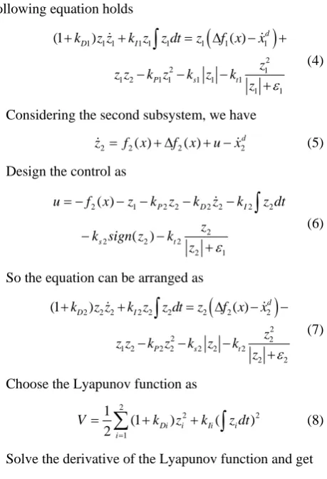
Considering the second subsystem, we have

2 2( ) 2( ) 2 d

z_& = f x + Δf x + −u x&

(5)

Design the control as

2 1 2 2 2 2 2 2

2

2 2 2

2 1

( )

P D I

s t

u

f x

z

k z

k

z

k

z dt

z

k sign z

k

z

ε

= −

− −

−

+

∫

&

(6)

So the equation can be arranged as

(

)

2 2 2 2 2 2 2 2 2

2

2 2

1 2 2 2 2 2 2 2 2

(1 _D ) _I ( ) d

P s t

k z z k z z dt z f x x

z

z z k z k z k

z

ε

+ + = Δ − −

− − −

+

∫

& &

(7)

Choose the Lyapunov function as

2

2 2

1

1 (1

)

(

)

2

i Di i Ii i

V

k

z

k

z dt

=

∑

+

_∫

(8)

Solve the derivative of the Lyapunov function and get

(

)

2

2 1

( ) d i

i i i Pi i si i ti

i i i

z

V z f x x k z k z k

z

ε

=

= Δ − − − −

+

∑

& _&

(9)

According to the assumption, there exist parameters

Pi

k

and

ksi

which is big enough such that

0

V&≤

(10)

Now, it is easy to prove that the system is stable.

IV. E

XAMPLE AND

S

IMULATION

Considering the above two-order system, we choose

1 1 1 1 1 2 1

2 2 2 2 1 2

( )

3 ,

( )

sin(

)

( )

4 ,

( )

cos(

)

f x

x

f x

x x

x

f x

x

f x

x

x x

=

Δ

=

+

=

Δ

=

(11)

Then the two order system can be written as

1 1 1 2 1 2

2 2 2 1 2

3 sin(

)

4 cos(

)

x

x x

x

x x

u

=

+

+ +

=

+

&

(12)

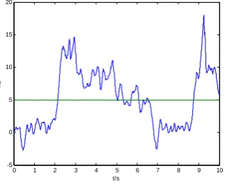
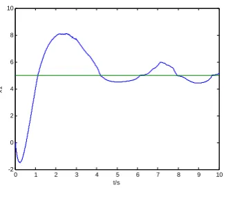
We define the desired signal as

1 5 d

x =

set the control

parameters as

kP1=5

,

kIi=ksi=kti=5

,

kP2 =20

， and

do the simulation with parameter as

kD1=0

and

1

D

k

=

respectively, the simulation result can be shown as

Fig.1 and Fig. 2. We can know from the above figures

that the overshoot can be reduced by adopting the

backstepping and PD hybrid control method, also the

performance of the system can be improved. But we

should also point out that if the derivative coefficient

does not increase properly, oscillation will be caused

(For example, we choose

kD1=kD2=1

to do the

simulation and the bad performance can be shown as Fig

3) or the system will become unstable (For example, we

choose

kD1=2,kD2 =1

to do the simulation and the bad

performance can be shown as Fig.4). Also, in some

situation, the demand for simulation algorithm will

become very strict if the pure derivative item is used. In

other hand, it is very difficult to get some derivative

signals in many actual systems, so we will consider

adopting a filter derivative to take place the pure

derivative.

(3)

0 1 2 3 4 5 6 7 8 9 10 -2 0 2 4 6 8 10 12 14 t/s x1

Figure 4. Curve of x1(kD1=2,kD2=1)

V. P

ROOF OF

F

ILTER

D

ERIVATIVE

M

ETHOD

Considering the above system

1 1 1 1 2

2 2 2

( )

x

f x

x

f x

u

=

+ Δ

+

=

+ Δ

+

&

(13)

We define

1 1 1 d

z

= −

x

and the first subsystem can be

written as

1 1

( )

1 1

( )

2 1 d

z

&

=

f x

+ Δ

f x

+

x

−

x

&

(14)

Design a virtual control as

2 1 1 1 1 1 1

1 1

1 1 1 1 1

1 1

( )

1 ( )

d P D

I s t

s

x

f x

k z

k

z

s

z

k

z dt

k sign z

k

z

τ

ε

= −

−

+

−

+

∫

(15)

where

1 1 s s

τ

+

is a filter which is used to get an

approximate derivative of the error

2

1 1

0,

2 1 1 2

z J

L J z

s s

τ

= = ≥ =

+ +

(16)

Then we have

τ

L&+ =L J

and solve the derivative we

get

2 2

1 1 1 1 1

2 1

1 1 1

2 1 2 1

z

L J V z

s

z sz

z z z

s s

τ

τ τ

τ

= − = − + ⎡ ⎤ ⎡ ⎤ = _⎢ − _⎥= _⎢ _⎥ + + ⎣ ⎦ ⎣ ⎦ &

(17)

Design

2 2 2 d

z =x −x

then the following equation holds

(

)

2 1 1 1 1 1 1 1

1

2

2 1

1 1 1 1 2 1 1 1 1 1

1 1 1 2 1 ( ) D I d

P s t

k z

z z k z z dt

s

z

z f x x z z k z k z k

z

τ

ε

′ ⎛ ⎞ + _+⎜ _⎟ + ⎝ ⎠ = Δ − + − − − +

∫

& &

(18)

Considering the second subsystem

2 2( ) 2( ) 2 d

z_& = f x + Δf x + −u x_&

(19)

We design the control as

2 1 2 2 2 2

1 2

2 2 2 2 2

2 1

( )

1 (

)

P D

I s t

s

u

f x

z

k z

k

z

s

z

k

z dt

k sign z

k

z

τ

ε

= −

− −

−

+

−

+

∫

(20)

Then the system can be arranged as

(

)

2 2 2 2 2 2 2 2

2

2 2

2 2 2 1 2 2 2 2 2 2

2 2 1 2 1 ( ) D I d

P s t

k z

z z k z z dt

s

z

z f x x z z k z k z k

z

τ

ε

′ ⎛ ⎞ + _+⎜ _⎟ + ⎝ ⎠ = Δ − − − − − +

∫

& &

(21)

And the Lyapunov function can be chosen as

2 2 2 2 1

1 (

)

2

1

i

i Ii i Di

i i

z

V

z

k

z dt

k

s

τ

=

⎛

⎞

=

_⎜

+

_⎟

+

⎝

⎠

∑

∫

(22)

The derivative of Lyapunov function can be computed

as

(

)

2

2 1

( ) d i

i i i Pi i si i ti

i i i

z

V z f x x k z k z k

z

ε

=

= Δ − − − −

+

∑

& _&

(23)

According to the assumption, there exist two big

enough parameters

kPi

and

ksi

such that

0

V&≤

(24)

So it is easy to prove that the system is stable.

VI. E

XAMPLE AND

S

IMULATION

Now the above system is used to do the simulation and

we set

1 1 1 1 1 2 1

2 2 2 2 1 2

( )

3 ,

( )

sin(

)

( )

4 ,

( )

cos(

)

f x

x

f x

x x

x

f x

x

f x

x

x x

=

Δ

=

+

=

Δ

=

(25)

then the second order system can be written as

1 1 1 2 1 2

2 2 2 1 2

3 sin(

)

4 cos(

)

x

x x

x

x x

u

=

+

+ +

=

+

&

(26)

Define the desired value as

1

5

d

x

=

and use the

backstepping and filter derivative hybrid control method,

and choose the control parameters

as

k

P1

=

5 ,

k

Ii

=

5 ,

k

si

=

k

ti

=

5 ,

k

P2

=

20 ,

1

2

1

0.001

D

(4)

0 1 2 3 4 5 6 7 8 9 10 0

1 2 3 4 5 6

t/s

x1

0 1 2 3 4 5 6 7 8 9 10 0

1 2 3 4 5 6

t/s

x1

0 1 2 3 4 5 6 7 8 9 10 -5

0 5 10 15 20

t/s

x1

0 1 2 3 4 5 6 7 8 9 10 0

1 2 3 4 5 6 7 8

t/s

x1

0 1 2 3 4 5 6 7 8 9 10 0

1 2 3 4 5 6

t/s

x1

improve the performance of the system compared with

pure derivative method.

Considering that we further increase the uncertainties

of the system, we choose

2

( )

2

cos(

1 2

)

1

f x

x

x x x

Δ

=

and use

pure derivative to do the simulation. Through a series of

simulations, we found a better one with parameters

as

k

D1

=

0.5,

k

D2

=

1 , and the simulation result can be

shown as Fig 6. It is obvious that if we want to reduce the

oscillation and make the curve smooth, we need to

increase the derivative coefficients. But the increase of

the derivative caused the system to be unstable

unexpectedly, which can be shown as Fig 7 where the

parameters are chosen as

k

_D₁

=

2,

k

_D₂

=

1 .

Later, used the filter derivative algorithm and chose

parameters as

k

D1

=

2,

τ

1

=

0.001 ,

k

D2

=

1,

τ

2

=

0.1 , the

control effect is not very good, which can be shown as

Fig 8. And we changed the parameters as

1

5,

1

0.001

D

k

=

τ

=

and

k

D2

=

3,

τ

2

=

0.1 , and the

simulation result can be shown as Fig9. Also, the

parameters can be chosen in a big interval, and the

possibility that the system become unstable is reduced.

(5)

0 1 2 3 4 5 6 7 8 9 10 -2

0 2 4 6 8 10

t/s

x1

VII. C

ONCLUSIONS

Above of all, the main contribution of this paper can be

concluded as following points. First, a novel type of filter

derivative method was introduced to robust backstepping

design. Second, the relationship between transfer function

(an important concept in classic control theory) and

Lyapunov function (one of the most popular concept in

modern control theory) was established. What is very

different from other papers is that detailed and elaborate

simulations were done in this paper to research the

problem that how much uncertainties and how big an

amplitude of uncertainties can be solved by this filter

derivative method.

At last, the paper also shows some situations that the

proposed new method can not cope with and the reasons

are given to explain the result. Also, it points out our

future research field.

A

CKNOWLEDGMENT

The authors wish to thank their friend Heidi in Angels

(a town of Canada) for her help , and thank Amado for

his many helpful suggestions.

R

EFERENCES

[1] Hao Lei,Wei Lin，Universal adaptive control of nonlinear systems with unknown growth rate by output feedback， Automatica 42 (2006) 1783-1789

[2] Hao Lei,Wei Lin，Adaptive regulation of uncertain nonlinear systems by output feedback: Auniversal control approach , Systems & Control Letters 56 (2007) 529– 537 [3] Swaroop D, Gerdes J C, Yip P P, Hedrick J K. Dynamic

surface control of nonlinear systems. In: Proceedings of the American Control Conference. Albuquerque, New Mexico: IEEE, 1997. 3028-3034

[4] Swaroop S, Hedrick J K, Yip P P, Gerdes J C. Dynamic surface control for a class of nonlinear systems. IEEE Transactions on Automatic Control, 2000, 45(10): 1893-1899

[5] Zhang, T., Ge, S.S. & Hang, C.C. Adaptive neural network control for strict-feedback nonlinear systems using backstepping design. Automatica, Vol. 36. No. 12 (2000) 1835-1846

[6] Chiman Kwan and F. L. Lewis. Robust backstepping control of nonlinear systems using neural networks. IEEE Transactions on systems, man and cybernetics,Vol. 30. No. 6 (2000) 753-766

[7] Junwei Lei, Xinyu Wang, Yinhua Lei, How many parameters can be identified by adaptive synchronization in chaotic systems? [J] Physics Letters A， Volume 373, Issue 14, 23 March 2009, Pages 1249-1256

[8] Junwei Lei, Xinyu Wang, Yinhua Lei, A Nussbaum gain adaptive synchronization of a new hyperchaotic system with input uncertainties and unknown parameters, [J] Communications in Nonlinear Science and Numerical Simulation, Volume 14, Issue 8, August 2009, Pages 3439-3448

[9] Xinyu Wang,Junwei Lei, Yinhua Lei,Trigonometric RBF Neural Robust Controller Design for a Class of Nonlinear System with Linear Input Unmodeled Dynamics[J]. Applied Mathmatical and Computation，185 (2007) 989 –1002

[10]Wang Xinyu, Lei Junwei, Design of Global Identical Terminal Sliding Mode Controller for a Class of Chaotic System,2006 IMACS Multiconference on Computational Engineering in Systems Applications(CESA ′2006), Tsinghua University Press,2006.10

[11]Xinyu Wang, Hongxing Wang, Hong Lei, Junwei Lei , Stable Robust Control for Chaotic Systems Based on Linear-paremeter-neural-networks, The 2nd International Conference on Natural Computation (ICNC'06) and the 3rd International Conference on Fuzzy Systems and Knowledge Discovery (FSKD'06), Sep 24-28, 2006, Xi-an, China

[12]GE S S，Wang C，Lee T H. Adaptive backstepping control of a class of chaotic systems[J]. Int J Bifurcation and chaos. 2000, 10 (5): 1140-1156

[13]GE S S, Wang C, Adaptive control of uncertain chus’s circuits[J]. IEEE Trans Circuits System. 2000, 47(9): 1397-1402

[14]Alexander L, Fradkov, Markov A Yu. Adaptive synchronization of chaotic systems based on speed gradient method and passification[J]. IEEE Trans Circuits System 1997,44(10):905-912

[15]Dong X. Chen L. Adaptive control of the uncertain Duffing oscillator[J], Int J Bifurcation and chaos. 1997,7(7):1651-1658

[16]Tao Yang, Chun-Mei Yang and Lin-Bao Yang, A Detailed Study of Adaptive Contorl of Chaotic Systems with Unknown Parameters[J] . Dynamics and Control. 1998,(8):255-267

[17]M.T. Yassen，Adaptive chaos control and synchronization for uncertain new chaotic dynamical system，Physics Letters A 350 (2006) 36–43

[18]H.Nijmeijer,M.Y.mareels.An observer looks at synchronization.IEEE Trans.on Circuits Syst.I.1997, (44):882-890

[19]M.T.Yassen.Chaos synchronization between two different chaotc systems using active control.Chaos,Solitons & Fractals.2005:23(4):131-140.

[20]H.N.Agiza,M.T.Yassen. Synchronization of Rossler and Chen chaotic dynamical systems using active control.Physics Letters A.2001,(278):191-197.

[21]Ming-chung Ho,yao-Chen Hung.Synchronization of two different systems by Using generalized active control. Physics Letters A.2002,(301):424-428.

(6)

[23]BemdaroM. An Adaptive approach to the control and synchronization of continuous time chaotic systems[J]. Int J Bifurcation and chaos. 1996，6(3):557-568.

[24]GE S S，Wang C，Lee T H. Adaptive backstepping control of a class of chaotic systems[J]. Int J Bifurcation and chaos. 2000, 10 (5): 1140-1156

[25] GE S S, Wang C, Adaptive control of uncertain Chua’s circuits[J]. IEEE Trans Circuits System. 2000, 47(9): 1397-1402

[26]Alexander L, Fradkov, Markov A Yu. Adaptive synchronization of chaotic systems based on speed gradient method and passification[J]. IEEE Trans Circuits System 1997,44(10):905-912

[27]Dong X. Chen L. Adaptive control of the uncertain Duffing oscillator[J], Int J Bifurcation and chaos. 1997,7(7):1651-1658

[28]Tao Yang, Chun-Mei Yang and Lin-Bao Yang, A Detailed Study of Adaptive Contorl of Chaotic Systems with Unknown Parameters[J] . Dynamics and Control. 1998,(8):255-267

[29]Oscar. Fuzzy control of chaos [J] . Int J Bifurcation and chaos. 1998.8(8): 1743-1747

[30]Liang Chen, Guanrong Chen, Lee Yang-Woo, Fuzzy modeling and adaptive control of uncertain chaotic systems[J]. Information Sciences. 1999, 121(1):27-37 [31]Liang Chen,Guanrong Chen.Fuzzy presictive control of

uncertain chaotic Systems using time series[J].Int J Bifurcation and chaos.1999,9(40:757-767.

[32]Chin Teng Lin.Controlling chaos by GA-based reinforcement learning neural network [J]. IEEE Trans On neural networks. 1999,10:846-859

[33]Gao Ping Jing et al. A simple global synchronization criterion for coupled chaotic systems. Solitons and fractals. 2003,(15):925-935

[34]Jianping Yan, Changpin Li. On synchronization of three chaotic systems. Chaos,Solitons and fracrals.2005,(23):1683-1688

[35]C.Sarasola,F.J.Torrealdea,A.D Anjou. Feedback synchronization of chaotic Systems[J].Int.J.Bifurcation and chaos.2003,13(1):177-191

[36]M.T.Yassen.Chaos synchronization between two different chaotc systems using active control.Chaos,Solitons & Fractals.2005:23(4):131-140

[37]H.N.Agiza,M.T.Yassen. Synchronization of Rossler and Chen chaotic dynamical systems using active control.Physics Letters A.2001,(278):191-197

[38]Ming-chung Ho, Yao-Chen Hung.Synchronization of two different systems by Using generalized active control. Physics Letters A.2002,(301):424-428.Jiang G.P., Tang K.S. A global synchronization criterion for coupled chaotic systems via unidirectional linear error feedback approach. Int. J. Bifurcation Chaos, 2002, 12(10):2239-2253

[39]Bu S.L., Wang S.Q.An algorithm based on variable feedback to synchronize chaotic and hyperchaotic systems. Physica D,2002,164:45-52

[40] Suykens. J.A.K, Robust nonlinear

H

∞synchronization of chaotic Lur’s system, IEEE Trans Circuit & System1997， 44(10):891-903

[41]Michele B, Donato C. Synchronization of hyper-chaotic circuits via continuous feedback control with application to secure communication. Int. J. Bifurcation and Chaos, 1998,8(10):2031-2040

[42]Alexander L.Fradkov, A Yu.Markov. Adaptive synchronization of chaotic system phased on speed gradient method and passification. IEEE Trans on Circuit Syst.(I),1997,44(10):905-912

[43]Young_Hoon Joo, Leang-San shieh, Guangrong Chen, Hybrid state-space fuzzy model-based controller with dual-rate sampling for digital control of chaotic systems, IEEE Trans on Fuzzy Syst.(I),1999,7(4):394-408

[44]Alexander Pogromsky, Henk Nijmeijer. Observer-based robust synchronization of dynamical systems. Int,J. Bifurcation and Chaos,1998,8(11):2243-2254

[45]E.M.Elabbasy,H.N.Agiza,M.M.El-dessoky.Adaptive synchronization of lv System with uncertain parameters. Chaos,solitons and fractals. 2004,(21):657-667

[46]M.T.yassen. Adaptive synchronization of Rosser and lü systems with fully uncertain patameters. Chaos,solitons and fractals.2005,(23):1527-1536

[47]Ju H.Park. Adaptive sysnchronization of Rossler system with uncertain Parameters.Chaos, solitons and fractals.2005,(22):1-6.

Yue Zhi was born in Zouping, Shandong province of China on Dec, 1982. He received the B.S. degree in Electronic Automation and received the M.S. degree in Guidance, Control and Navigation from Naval Aeronautical and Astronautical University, China, in 2005 and 2008 respectively.

Now he is a Ph.D. candidate of Control Science and Engineering, Naval Aeronautical and Astronautical University, China. His current research interests include actuator and sensor nonlinearities, robust control and isolation of nonlinear systems.

Junwei Lei was born in Chibi, Hubei province of China on 9th_{Nov, 1981. He} received the B. Eng degree in Missile Control and Testing and the Master Degree in Control Theory and Control Engineering from Naval Aeronautical Astronautical University， Yantai of China in 2003 and 2006 respectively. After that he continued his study there and received the Doctor degree in Guidance , Control and Navigation in 2010 .

He worked in NAAU as an assistant teacher in 2009 and became a lecture in 2010. His present interests are neural networks, chaotic system control, variable structure control and adaptive control.

Mr Lei studied in Canada Military Force and Language School in Base Bodern of Toronto from Jan to Jun in 2010.

Jinyong Yu was born in Haiyang, Shandong province of China in 1976. He received the B. Eng degree in Automation Engineering in Central South University in 1999 and received the Master Degree in Control Theory and Control Engineering from Naval Aeronautical Astronautical University， Yantai of China in 2002. He received the Doctor degree in Guidance, Control and Navigation from NAAU in 2006 respectively.