Discretization Model of Instantaneous Availability for Continuous-time Systems

Discretization Model of Instantaneous

Availability for Continuous-time Systems

Yi Yang1,2

1. Reliability and Systems Engineering School Beihang University

Beijing, P.R. China, 100191

2. China Astronaut Research and Training Center Beijing, P.R. China, 100191

[email protected]

Lichao Wang1 and Rui Kang2 Reliability and Systems Engineering School

Beihang University Beijing, P.R. China, 100191

[email protected] [email protected]

Abstract— In this paper, the instantaneous availability models in continuous and discrete time are proposed for the one-unit repairable systems with delay under exponential distributions. Prior to this, error analyses of sampling discrete distributions are given. Then, the numerical solutions for the continuous- time model and the discrete-time model are presented. The comparison of the solutions reveals that with the step length and sampling interval decreasing, the accuracy of the numerical model is much better. Also, in the same accuracy level, less computation time is needed to solve the discrete-time model. Hence, the discrete-time model is more feasible to analyze instantaneous availability. Finally an example is given to describe the application of the results.

Keywords- Instantaneous availability; Continuous-time model; Discrete-time model; Comparation analysis

I. INTRODUCTION

With the phenomenon of system instantaneous availability undulation in early stage of use, its research requirements are brought forward, that is not only various instantaneous availability models are established for the complex systems via ordinary and partial differential or integral equations, base on which, the existence and solvability of steady-state system availability are investigated [1-7], but also the mechanism of the system instantaneous availability undulation between [0,T] is studied. The analytic solution and high efficient numerical solution of the instantaneous availability are needed. However the solutions can be obtained only for a few systems with some special distributions, e.g., the exponential distributions. Because of very large computation scale, the computation involved in current corresponding numerical method is not applicable for engineering design. Hence, it is very necessary to find

some new approaches for solving instantaneous availability.

The phenomenon of availability undulation abounds in new equipment systems [8-10]. There are two main methods to get the instantaneous availability: probability methods and simulation methods. However, the instantaneous availability by simulation methods can not reflect the undulation mechanism.

In engineering applications, operation time and maintenance time of many repairable systems are discrete time [11-15]. For discrete-time system, its instantaneous availability has a very simple form, and is much easy to be computed. It is very available to obtain the numerical solutions for the case of discrete-time events [16]. However, in the continuous process case, the usual treatment is to discretizate the continuous models, and then to get the solution of the discrete models to approximate the original continuous solution. Can such a procedure achieve the ideal accuracy? This motivates the investigation in this paper.

In order to access the conclusion on whether the discrete-time models or the continuous-time ones are better in the sense of more accuracy and less computation, we compare and analyze the approximation errors between the numerical solutions of both the discrete and continuous cases and the accurate analytical solutions, respectively, for the systems obeying exponential distribution. The studies show that discrete-time models are much better than continuous ones and thus are much more applicable for the researches of instantaneous availability.

II. ERROR ANALYSES OF SAMPLING DISCRETE DISTRIBUTIONS

( )

t f

( )

sds F =

∫

t

0 , t≥0 (1) Let T be sampling period. In practical engineering, the start time of the repair for fault parts and the work after repair are all considered to occur in the sampling points, that is to say, the lifetime and repair time can be considered as discrete random variables X~ , the corresponding density function and distribution function are as follows

( )

{

(

)

}

( 1)

( )

1 k T

T _kT

f k =P kT≤X% < k+ T =

∫

+ f t dt

k=0,1,2,... (2)

( )

_∑

( )

=

= k

j T

T k f j

F

0

k=0,1,2,... (3a) or

( )

_∑

( )

= = k j T

T t f j

F

0

kT≤t<

(

k+1

)

T (3b)

Then for any t≥0, there must exist a number k, s.t.,

(

k

)

T

t

kT ≤ < +1 , so

( )

t F

( )

t f

( )

sds ( ) f

( )

sds F

(

( )

k T

) ( )

FkT

F k T

kT t

kT

T = ≤ = + −

−

≤

_∫

_∫

+ 1

0 1

{

_F

[

(

_k

)

_T

] ( )

_{F kT}

} ( )

_{H T}

N

k + − Δ

≤

∈ 1

max (4)

According to the definition of density distributions,

( )

t

f is a non-negative function on

[

0,+∞

)

and

( )

1

0 =

∫

+∞ f tdt

It is easy to get that

( )

0

0

T

H T ⎯⎯⎯→→

For a given ε0>0, there must exist a sufficiently small number T , s.t., H

( )

T ≤ε₀ . Therefore, it is reasonable that X~ be used to replace X.

III. NUMERICAL METHOD OF CONTINUOUS TIME MODEL

Let the system be composed by a single component and the fault time X and the time Y to repair after fault follow the general probability distribution F

( )

t and

( )

t

G , respectively. Considering the delays in repair process, suppose that the repair delay W follows general probability distribution W

( )

t . Assume that after the repair system is as good as new, and X and Y are independent. For simplicity, we assume that components are new in moment 0.

Reference [2] established single components of Markov repairable system availability model via the theory of renewal process. According to this, via using the theory of renewal process, the system availability model of one-unit- delay repairable systems can be obtained as follows.

( )

t R

( )

t A

(

t u

) ( )

dQu R

( ) ( ) ( )

t Qt At

A t *

0 − = +

+

=

_∫

(5)

where

( )

t F

( )

t

R =1− then

( )

t R

( )

t A

(

t u

) ( )

dQu R

( ) ( ) ( )

t Qt At

A t *

0 − = +

+

=

_∫

( )

_∫

(

) (

_∫

) (

_∫

) ( )

∫

+ − − −

−

= tf sds tAt u uwu s sf s v g vdvdsdu

0 0 0

0

1 Let

0

0 =

t , t1=t0+h, t2=t0+2h, …,tN =t0+Nh

where h>0 is the step. Note that there is an integration core. The rectangular formula [17] is applied.

( )

= −

_∫

j

( )

+

_∫

tj

( )

−

_∫

u

(

−

) (

_∫

s −

) ( )

j t

j f sds At u wu s f s vgvdvdsdu

t A

0 0 0

0 1

( )

_∑

(

)

_∫

(

) (

_∫

) ( )

∑

= = − − − + − ≈ j i t s i i j j i i i ds dv v g v s f s t w t t A h t f h

1 0 0

1 1

( )

_∑

(

)

_∑

(

) (

_∫

) ( )

∑

= = = − − − + − ≈ j i i l t l l i i j j i i l dv v g v t f t t w h t t A h t f h

1 1 0

1 1

( )

_∑

[

( )

]

_∑

[

( )

]

_∑

[

( )

] ( )

∑

= = = = ⎭⎬ ⎫ ⎩ ⎨ ⎧ ⎭ ⎬ ⎫ ⎩ ⎨ ⎧ _{− −} − + − ≈ j i i l l u j i uh g h u l f h h l i w h h i j A h ih f h

1 1 1

1 1

( )

_∑

[

( )

]

_∑

[

( )

]

_∑

[

( )

] ( )

∑

= = = = ⎭⎬ ⎫ ⎩ ⎨ ⎧ ⎭ ⎬ ⎫ ⎩ ⎨ ⎧ _{− −} − + − = j i i l l u j i uh g h u l f h l i w h i j A h ih f h

1 1 1

3

1 1

where

( )

j

j f t

f = , g_j =g

( )

t_j , w_j =w

( )

t_j , j=1,2,... Let numerical solution of instantaneous availability be

( )

j

j At

A = , j=1,2,...

Then the instantaneous availability of the iterative approximation is

(

)

∑

∑

∑

∑

= − = − = − = ⎭⎬ ⎫ ⎩ ⎨ ⎧ ⎥ ⎦ ⎤ ⎢ ⎣ ⎡ + − = j i i l l u u u l l i i j j i i

j h f h A w f g

A

1 1 1

3

1

1 (6)

IV. THE DISCRETE-TIME MODEL DESCRIPTION Define system state:

( )

( )

( )

⎪ ⎩ ⎪ ⎨ ⎧ = = = 2 1 0 Z k Z k Z k . at repaired being ; at waiting -reparation ; at normal t t t

k =0,1,2,...

Let failure function and repair rate function be λ

( )

k and

( )

k

μ , respectively. Denote

( ) {

k =PW=k|W≥k

}

ρ k=0,1,2,...

Let P0

( )

k,j , P1

( )

k,j and P2

( )

k,j be the probability of the system reach the state 0, 1, and 2 at time k,

respectively. i.e., whenj =0,1,...,k−1

( )

{

( )

(

)

(

)

}

( )

{

( )

(

)

(

)

}

( )

{

( )

(

)

(

)

}

0 1 2

, ... 0, 1 1

, ... 1, 1 2

, ... 2, 1 0

P k j P Z k Z k j Z k j P k j P Z k Z k j Z k j P k j P Z k Z k j Z k j

⎧ = = = − = − − = ⎪⎪ _{= = = − = − − =} ⎨ ⎪ = = = − = − − = ⎪⎩

whenj=k,

( )

{

( )

( )

}

( )

{

( )

( )

}

( )

{

( )

( )

}

0 1 2

, ... 0 0

, ... 0 1

, ... 0 2

P k k P Z k Z P k k P Z k Z P k k P Z k Z

⎧ = = = =

⎪⎪ _{= = = =}

⎨

⎪ _{= = = =}

When,k< j,

( )

, 0

0 k j =

P ,P₁

( )

k,j =0,P₂

( )

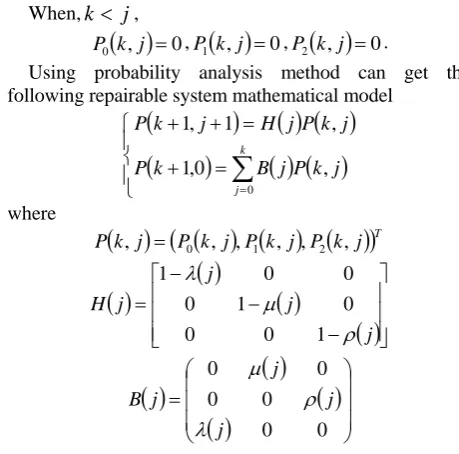
k,j =0.

Using probability analysis method can get the following repairable system mathematical model

(

)

( ) ( )

(

)

( ) ( )

⎪ ⎩ ⎪ ⎨ ⎧ = + = + +

∑

= k j j k P j B k P j k P j H j k P 0 , 0 , 1 , 1 , 1 where

( )

(

( ) ( ) ( )

)

T

j k P j k P j k P j k

P , = 0 , , 1 , , 2 ,

( )

( )

( )

( )

⎥⎥ ⎥ ⎦ ⎤ ⎢ ⎢ ⎢ ⎣ ⎡ − − − = j j j j H ρ μ λ 1 0 0 0 1 0 0 0 1

( )

( )

( )

( )

⎟⎟ ⎟ ⎠ ⎞ ⎜ ⎜ ⎜ ⎝ ⎛ = 0 0 0 0 0 0 j j j j B λ ρ μ

New system is always assumed to be available, namely

( )

0,0 1

0 =

P , P₁

( )

0,0 =0, P₂

( )

0,0 =0. The system availability for the instantaneous is

( )

0 0

( )

,

k j

A k =

∑

₌ P k j (7)

V. COMPARISIONS OF THE NUMERICAL AND ANALYTICAL SOLUTIONS

For the solvability of the systems, we consider the Markov repairable systems [18] with fault time, repair time after fault and the repair delay time following the exponential distributions with respect to

λ

,

μ

and

ρ

, respectively. Define the system state as

( )

( )

( )

⎪ ⎩ ⎪ ⎨ ⎧ = = = 2 1 0 Z t Z t Z t t t t at repaired being at waiting -reparation at normal Let

( )

t P

{

Z

( )

t j

}

Pj = = , j=0,1,2 Then

( )

( )

( )

( )

( )

( )

⎟⎟ ⎟ ⎠ ⎞ ⎜ ⎜ ⎜ ⎝ ⎛ ⎥ ⎥ ⎥ ⎦ ⎤ ⎢ ⎢ ⎢ ⎣ ⎡ − − − = ′ ⎟ ⎟ ⎟ ⎠ ⎞ ⎜ ⎜ ⎜ ⎝ ⎛ t P t P t P t P t P t P 2 1 0 2 1 0 0 0 0 μ ρ ρ λ μ λ

( ) ( ) ( )

(

P₀ t,P₁ t,P₂ t

)

|_t=0=

(

1,0,0

)

. The instantaneous availability

( )

t P

( )

t A = ₀

Let λ=0.2, μ=2, ρ=3.6. Then

( )

52 45 4 1 13

5 2.6 ₊ 3.2 ₊

= − t − t

e e

t

A , t≥0

The experimental environment is: PC Celeron (R) 1.80 GHz CPU, 0.99 GB RAM, Windows XP, simulation software for MATLAB7.3. From figure 1, it is easy to see that the smaller the step is, the smaller the error is. For the fixed step, the error in the initial phrase is acceptable.

However, with the time goes on, the error increases gradually. This is resulted from that the convolution makes the computation involving in all the results in former steps. The error is thus accumulated that even makes the availability greater more than 1. This contradicts with the common sense. Hence, to obtain a more satisfactory solution, the step must be taken very small. This will result in the great computation cost.

0 1 2 3 4 5 6 7 8 9 10 0.85 0.9 0.95 1 1.05 1.1 1.15 1.2 time a v a ila b ili ty accurate availability step h=0.05 step h=0.02

Fig. 1 Comparison between numerical and analytical solutions in different steps continuous-time case

0 1 2 3 4 5 6 7 8 9 10 0.85 0.9 0.95 1 time a v a ila b ili ty accurate availability sampling period T=0.05 sampling Period T=0.01

Fig2. Comparison between numerical and analytical solutions in different sampling period discrete-time case

From figure 2, it is easy to see that the smaller the sampling period is, the smaller the error is. For the fixed step, the error in the initial phrase is acceptable. However, with the time goes on, the error does not increase gradually. This differs from the continuous case.

Table 1 CPU time consuming in different steps

step

h

0.05 0.02

CPU time (s) 2.3438 74.9219 Table 1 and table 2 gives the computational time. Choose step h =0.02 and sampling period T=0.05, we can see that with the time goes on, the error in discrete-time model is obviously much better than that in continuous-time case (see Figure 1 and Figure 2).

Table 2 CPU time consuming in different sampling period

sampling period

T

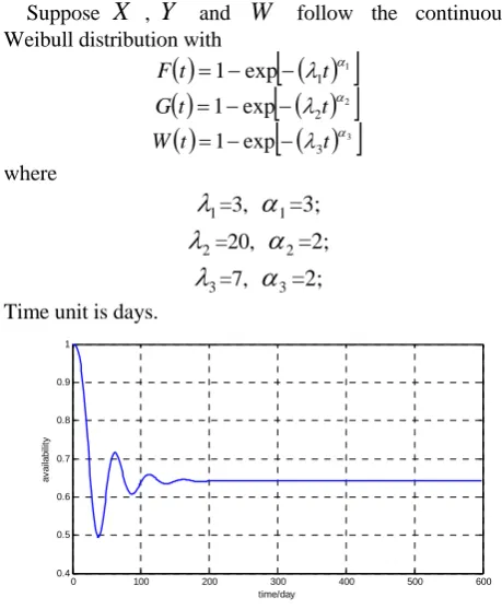
0.05 0.01

Suppose

X

,

Y

and

W

follow the continuous Weibull distribution with

( )

[

( )

1

]

1

exp

1 λt α

t

F = − −

( )

[

( )

2

]

2 exp

1 λ tα

t

G = − −

( )

[

( )

3

]

3 exp

1 λ t α

t

W = − −

where

1

λ

=3,

α

₁=3;

2

λ

=20,

α

₂=2;

3

λ

=7,

α

₃=2; Time unit is days.

0 100 200 300 400 500 600 0.4

0.5 0.6 0.7 0.8 0.9 1

time/day

a

v

a

ila

b

ilit

y

Fig. 3 Approximate instantaneous availability

The continuous-time system can be transformed into discrete-time system by sampling method. Let

T

=0.01 day. The corresponding instantaneous availability is obtained, as shown in figure 3. Under appropriate sampling period, the availability undulation of the approximate discrete-time system can be used to reflect the characteristics of instantaneous availability for the real system.

VI. CONCLUSIONS

In this paper, the numerical computation and accuracy of the discrete-time instantaneous availability model single- unit-reparable systems following exponential distribution are investigated. The studies reveal that the continuous-time models are not better in accuracy and computation complexity when the numerical algorithms are exacted. The longer the time interval is considered, the worse the computational errors accumulation becomes. In an appropriate sampling rate, it is shown that the solutions of the discrete-time models are almost as same as the accurate analytic solution. Hence, the discrete-time model can be a much better simplified substitution of continuous-time models for the studies of instantaneous availability. This is very significant for us to investigate the phenomenon of the undulation of instantaneous availability.

VII. ACKNOWLEDGMENT

The authors wish to thank Prof Y. Zou of Nanjing University of Science and Technology for his valuable suggestions. This work was supported in part by grant from National Natural Science Foundation of China

(61104132) and Director of the Fundation (SJ201002). Finally, the authors would like to thank the Associate Editors and anonymous reviewers for their insightful comments.

REFERENCES

[1] Barlow R E, Proschan F. Mathematical Theory of Reliability [M]. New York: Wiley, 1965.

[2] Cao J, Cheng K. Introduction of Reliability [M]. Beijing: Science Press, 1986.

[3] Sherwin D J. Steady-state Series Availability [J]. IEEE Transactions on Reliability, 2000, 49(2): 131~132. [4] Zeng S, Zhao T, Zhang J, et al. Course of System

Reliability Design tutorial [M]. Beijing: Beihang University Press, 2001.

[5] Xu H, Guo W, Yu J, et al. The Asymptotic Stability of a Series Repairable System [J]. Acta Mathematicae Applicatae Sinica, 2006, 29(1):46~52.

[6] Cassady C R, Lyoob I M, Scheider K, et al. A Generic Model of Equipment Availability under Imperfect Maintenance [J]. IEEE Transactions on reliability, 2005, 54(4): 564~571.

[7] Mi J. Limiting availability of system with non- identical lifetime distributions and non- identical repair time distributions [J]. Statistics & Probability Letters 2006, 76: 729~736.

[8] Wang L, Yang Y, Yu Y, et al. Analysis of matchable problems based on system availability [J]. Journal of Systems Engineering, 2009, 24(2):253-256.

[9] Wang L, Yang Y, Yu Y, et al. Undulation analysis of instantaneous availability under discrete Weibull distributions [J]. Journal of Systems Engineering, 2010, 25(2):277-283.

[10] Wang L, Yang Y, Zou Y, et al. Minimal availability variation design of repairable system under discrete Weibull distribution [J].Control Theory& Applications, 2010, 27(5):575-581.

[11] Wang J. Reliability Analysis of Discrete-Time Serial System [J]. Journal of Northern Jiao tong University, 2001, 25(6): 81-84.

[12] Wang L, Yang Y, Zou Y. Optimal Preventive Maintenance Interval Model of Discrete Time System. Journal of Nanjing University of Science and Technology, 2009, 33(1): 7-11.

[13] Xue Y, Cao J. Discrete Time Series Repairable System Operating Under Changing Environment [J]. Journal of System Science and Mathematical Science, 2003, 23(2): 242-250.

[14] Xue Y, Cao J. Discrete Time One-Unit Repairable System Operating Under Changing Environment [J]. Journal of System Science and Mathematical Science, 2006, 26(2): 178-186.

[16] Yang Y, Wang L, Zou Y. Reliability Analysis of Discrete-time One-unit Repairable System [J], Journal of Nanjing University of Science and Technology , 2008, 329(4): 393-396.

[17] Huang L, Hong Y, Jin X, et al. A Calculation Method of

Availability of Repairable Units Based on Integral Equation [J]. Development & Innovation of Machinery & Electrical Products, 2007, 20(5):25-27.