best practice design guide Deploying Very High Density Wi- Fi DESIGN AND CONFIGURATION GUIDE FOR STADIUMS

(1)

Deploying

Very High

Density Wi-‐Fi

DESIGN AND CONFIGURATION

GUIDE FOR STADIUMS

(2)

Intended Audience

This document addresses factors and concerns related to very dense Wi-‐Fi environments such as stadiums. Because venues can differ radically, it is impossible to develop a single approach that adequately addresses all potential design and installation issues.

This document is written for and intended for the sole use of system integrators or professional services with significant background in Wi-‐Fi design and 802.11/wireless engineering

principles. This document is not appropriate for end-‐user design work without the help of an experienced professional services team.

(5)

Overview

As more Wi-‐Fi capable devices enter the market the average number of devices in any given area of a network increases. In the case of extremely dense venues such as stadiums or exhibit halls, these very dense populations can introduce significant stress on the network and require specific design considerations. There are a number of factors that can impact a very high density environment, including:

• Performance requirements • Number and density of APs • Number and density of clients • Wi-‐Fi capabilities of clients • Current RF environment • AP hardware

• AP mounting

Each of these conditions can potentially cause severe network degradation. This document addresses ways to mitigate these negative performance issues and increase overall

performance and network stability. There are many types of high-‐density environments and each may have its own unique requirements. This guide will focus exclusively on very dense environments such as those found in stadiums, arenas, large exhibit halls, etc. These environments have unique properties that are not found in other Wi-‐Fi deployments.

Note: other high density applications such as school classrooms and smaller convention center venues should use the “Best Practices: High Density Design Guide” from Ruckus Wireless instead.

The rest this document will examine each of these points in-‐depth and offer guidelines and suggestions for optimized very high-‐density design configuration with Ruckus wireless equipment. Where needed, specific configuration commands are documented for step-‐by-‐step configuration instructions.

(6)

Design Process Overview

Although specifics can vary, any design team is expected to be familiar with the following process and tools. These are required for a successful design and deployment.

Discovery

Initial customer meetings to determine:

• Venue specific documentation (CAD drawings, photos, cabling maps, etc.) • Expected capacity (users)

• Supported applications

• Key Performance Indicators (KPIs) • Coverage areas

• Client devices that need to be supported

On-‐site Visit

First physical visit to the site to determine:

• Walkthrough of coverage areas

• Confirm accuracy of received documentation

• Confer with venue representative on places that cannot be used for mounting positions and other potential issues (I know you said something above but this is more specific)

• Gather additional intelligence, i.e. where are the VIPs and what type of events occur there. What type of events would need special wireless services or to have the Wi-‐Fi turned off because of exhibitors’ equipment running on same frequencies.

Wi-‐Fi Design

All of the information previously gathered is used to do a simulation of the venue. This is used to create an initial design including:

• Bill of materials (BOM) for the wireless network

• BOM for supporting equipment (wired network build-‐out, conduit, wire hangers, etc.)

• Installation locations for equipment

• Hardware/workers required for installation (cherry pickers, etc.) • Estimated coverage and capacity report

(7)

Installation

After the design is approved, the equipment is procured and installed at the venue. This needs to be coordinated with the venue manager as to not interfere with the primary functions of the venue. Sports teams may have strict guidelines as to when access will be granted and when workers may not be in the building. Also there will be a requirement for the project completion. This schedule will be very important to define so that all parties will have their portions of the project ready for installation at time required. Any delays here can cause long delays in completing the project and cause friction with the venue management or owner.

RF Survey

Once the equipment is installed, the design model is verified against the deployed environment. This step consists of a follow-‐up visit to site to conduct actual RF testing and initial design validation.

Testing & Acceptance

This consists of on-‐site validation and confirmation of the initial design goals and success criteria.

(8)

Coverage vs. Capacity in Very

Dense Environments

Why Are Stadiums Different?

Most Wi-‐Fi networks are designed for offices, public buildings, schools, warehouses, hospitals, etc. These sites typically require a wireless network that is optimized for good capacity with a fairly large coverage area for each AP.

Very dense venues such as stadiums have very different requirements that break this model. These deployments feature a very large number of people and devices within a large but highly concentrated area where much of the network, users and Access Points are LOS to each other. What works in an office will definitely not work in a stadium. The key difference is capacity. Very high-‐density designs require new thinking, see Table 1.

Coverage Capacity

Number of APs Prefer low Prefer high

Limiting factor Path loss Interference

Obstacles Bad Good

RF frequency Lower is better Higher is better

Antenna pattern Omni is better Sector is better

AP placement Higher is better Lower is better

Design metric SNR area SINR area

Table 1

(9)

© 2012 Ruckus Wireless, Inc Best Practices v1.0 8 The most significant factor in very dense deployments is the need to support a large number of people packed very closely together. The large number of people and devices requires a large number of APs that are also close together. But placing that many APs so close together brings its own challenges; namely increased RF interference.

RF interference is a huge driver with immense impact on the final design. Fortunately, there are some strategies to help mitigate its effect. These include:

• Increased use of 5 GHz RF spectrum for less interference and more channels (capacity)

• Shrink AP cell sizes as much as possible

• Increase AP count, but only to the extent of estimated capacity (more is not better). • Understand required capacity to avoid over-‐building network (increases

interference unnecessarily) • High frequency re-‐use • Via directional antennas

• Structural separation and attenuation • Non-‐traditional 2.4 GHz channel plans

• RF simulation tools to optimize design before final design or installation • Configuration optimizations

• Adaptive algorithms to handle changing RF conditions without manual intervention

5 GHz: The Future of Wi-‐Fi

Increased use of 5 GHz is on the rise; newer clients are usually dual-‐band meaning they can use either 2.4 GHz or 5 GHz. This is true even of newer smartphones as well as tablets and laptops. This trend is expected to accelerate as device vendors position themselves to

support 802.11ac, which only operates in the 5 GHz spectrum. All of this has positive implications for Wi-‐Fi.

5 GHz is preferred for several reasons, not least of which include a wider frequency spectrum. This band typically offers 6 to 7 times the bandwidth of 2.4 GHz in most countries. With a larger amount of spectrum comes more non-‐overlapping channels. As the number of available channels increases, the opportunity for channel re-‐use goes up. Channel re-‐use is the frequency with which a single channel can be used again by other APs without causing undue co-‐channel interference. Unlike 2.4 GHz which only has 3 non-‐overlapping channels (and therefore a frequency re-‐use factor of 3), 5 GHz supports re-‐use factors of 4, 7, 9 or even 12 or higher. Smaller channels reused more times will give more capacity than larger channels reused less often.

Higher channel re-‐use has huge implications for very dense deployments because it reduces the limiting factor of co-‐channel interference. A higher re-‐use factor increases the number of APs, which is necessary to meet capacity demands. This equates to 8 – 10 times increase in Mbps/m2 over the 2.4 GHz band.

(10)

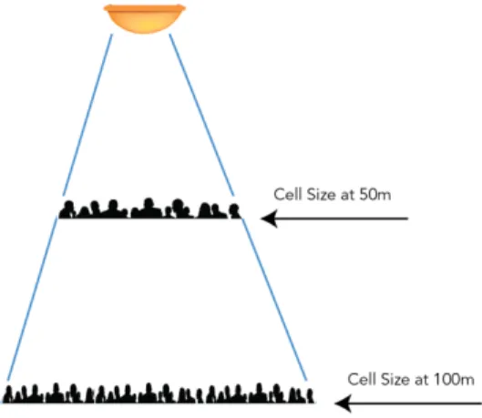
Decreasing Cell Size

Each AP in a wireless network represents additional capacity. Large venues demand very high capacity and therefore far more APs than would be required for a strictly coverage-‐oriented model. Therefore, the goal of a very dense deployment is very small AP coverage (cell) sizes. Keeping cell size to a minimum requires placing APs as close to the users as possible and keeping them isolated from other APs. Isolation is achieved via non-‐overlapping channels, structural isolation (attenuation or blocking of signals) and directional antennas to keep the coverage area small.

Breaking Away from Traditional 2.4 GHz Channel Plans

Although 5 GHz is becoming more popular, 2.4 GHz-‐only clients will be around for a long time and must be supported. But very dense deployments are not 2.4 GHz friendly due to the requirement for high channel re-‐use and minimal interference. Traditional 3 or 4 channel plans are not good enough.

2.4 GHz is vulnerable to RF interference both Wi-‐Fi and non-‐802.11. In an urban environment, the vast majority of interference comes from neighboring Wi-‐Fi networks. These networks prefer 3 channel plans (1, 6 and 11), which are the only non-‐overlapping channels available in this band. There can also be interference from the concession areas because of the use of microwaves for food preparation.

It is very easy to dismiss these neighboring networks because they appear usually appear at very weak signal strengths in the target venue. But lower power has worse implications for new 2.4 GHz deployments. The reason is most of these APs are using the minimum

transmission rate (1 Mbps) for beacon and management frames. Therefore there is a constant sea of low power, low speed traffic almost everywhere.

This traffic is completely irrelevant to the venue network and is received at a very low power. The simple solution is to increase power on the venue APs; that is easily done. But higher power doesn’t solve the intrinsic problem with co-‐channel interference: preambles. A preamble is the first part a frame transmitted by a Wi-‐Fi client. It is used by a station to tell the AP it’s about to transmit. It does not contain much useful information but it is required by the standard. In the 2.4 GHz band there is a “legacy” long preamble and a shorter preamble. All 802.11g 2.4 GHz stations are required to support both. Not only do long preambles take longer to transmit, they are always sent at the lowest possible speed (1 Mbps).

Traditional networks can only solve this problem by trying to be on a different non-‐overlapping channel. But since there are only 3 in the 2.4 GHz band, this is not realistic. A better solution is to make use of the other channels. These channels do overlap with traditional plans but have a huge benefit: clients that are on these channels do not hear stations on channels 1, 6 or 11. A client on channel 7 does not need to pay attention to a neighboring network transmitting on channels 6 or 11. It freely ignores these irrelevant preambles.

(11)

RF Simulations

Unlike most other (indoor) deployments, large venues incur significantly higher installation costs. A stadium does not have as many available installation locations as an office and they are much more difficult to reach. Because of this, there is a much higher incentive to know exactly where to put the AP before it is installed. Cherry pickers are expensive to procure and use; installing new cable runs is also costly compared to a more standard indoor environment. Many venues require that all cabling is placed in conduit which further increases cost and makes proper the next step so important.

The only way to solve this problem is with the use of sophisticated RF simulation software used by knowledgeable designers and engineers. These predictive models help determine the most advantageous locations before a single AP is deployed. This reduces the possibility of later costly adjustments.

Configuration Optimizations

Overall performance is further improved with the use of configuration adjustments that help with the unique requirements of large venues. These include:

• OFDM only in the 2.4 GHz band (drop support for 802.11b clients) • Disable background scanning by APs

• Enable RTS-‐CTS to mitigate collisions

• Limit the number of SSIDs as much as possible to reduce management traffic and overhead

• Disable any service that may potentially deny service such as WIPS

What About Reducing Transmit Power?

A common tactic used to shrink AP cell size and reduce interference is lowering the AP transmit power. But this rarely has the desired effect. Reducing power might lower contention on the medium, but there are better ways to do this. Ruckus products use a dynamic, adaptive antenna array that automatically steers around interference and does not transmit extraneous RF outside the targeted client area.

Lower power also doesn’t reduce the signal to self-‐interference ratio. Even worse, it is guaranteed to reduce to the signal to noise ratio from neighboring interference. This only makes things worse for clients, which will now have a harder time hearing the AP. Reducing power also lowers the transmit speed to the clients. This means they spend more time on the air listening; further reducing capacity.

(12)

Capacity Optimization

Capacity is critical for large venues. Incorrectly estimating capacity can result in poor performance and coverage holes from insufficient APs. On the other hand, overestimating the number of APs does not make clients perform better it just increases interference

unnecessarily. This ultimately reduces capacity. Capacity is a key part of RF simulation software such as iBwave or Motorola’s Enterprise Planner. These packages include capacity estimation metrics – in particular, the percentage of coverage area that provides a SINR of at least 25 dB or greater and this is key.

This percentage should be verified for individual sections of the venue and then iterated across the entire coverage area. Every area must be accounted for in the design before a final signoff.

Summary

This section described key elements of design vital for deployment of very large and dense Wi-‐ Fi networks. The rest of this document delves into these topics in greater detail and

explanation. Unlike a standard indoor deployment, large venues must meet all of these requirements and have them carefully validated at every step in the process. Each step is critical because errors in the design are magnified and have much larger impacts than other most other wireless deployments.

(13)

Performance Requirements

Understanding the Applications

The first thing that any high-‐density design should determine and document are the key performance metrics. These applications can include general internet access, voice (VoIP), video, food service, ticketing, just to name a few. The service requirements for these

applications define the minimum device requirements for successful operation. These are vital to calculate the number of devices per AP and, from that, the number of required APs.

Other Performance Factors

The second significant part of the design is the number of APs required to meet the KPIs. This number is critical but cannot be determined based on KPIs alone. There are several other factors that will impact overall performance, AP capacity and consequently the number of APs. These factors include:

• Number of devices expected on the Wi-‐Fi network

• Type of device that will be utilized, scanners, handsets, tablets, etc. • Device capability

• RF interference

(14)

Reference Design Example

The easiest way to show how these factors can be derived and used is by example. The rest of this document will use a 20,000-‐seat stadium as a reference design. As with any high-‐density venue, specific deployments may have slightly different requirements. However the principles outlined here are applicable for any size venue.

Venues rarely have a single application and a single type of user. Instead, there are typically many groups with specific requirements, applications and coverage needs. This document addresses the most common or significant criteria for a successful deployment.

Key Performance Indicators (KPI)

KPI metrics are the ultimate measure of a successful deployment. Therefore they should be as accurate as possible. Under estimating requirements will result in poor performance and a design that does not meet required needs. Over estimating could potentially result in a network that is so large it interferes with itself and reduces overall capacity.

Common KPIs include:

• Type of applications that will be supported

• Minimum bandwidth required to satisfy supported applications • Minimum, maximum and average number of Wi-‐Fi enabled devices • The expected number of active Wi-‐Fi devices at peak traffic time. • Maximum latency and jitter tolerated

• Service area definition

(15)

Application Types and Metrics

Supported applications may vary depending on the venue and on the intended audience. For example, guest attendees are usually offered web and email while venue employees use ticketing or point of sales (POS) applications. Table 2 illustrates common applications as well as their specific performance requirements:

Supported Applications by Group/Application Group Applications Minimum

Bandwidth Max Latency Tolerance

Guests/attendees Web access Email Video playback ~ 300 Kbps ~ 200 Kbps ~ 500 Kbps Medium High Medium Ticketing Ticket scanning < 200 Kbps High

Services

(Restaurants, etc.) POS Determined by application Determined by application Venue staff Web access

Email VoIP ~ 300 Kbps ~ 200 Kbps ~100 Kbps Medium High Low Guests/attendees Web access

Email Video playback ~ 300 Kbps ~ 200 Kbps ~ 500 Kbps Medium High Medium Ticketing Ticket scanning < 200 Kbps High

Services

(Restaurants, etc.) POS Determined by application Determined by application Venue staff Web access

Email VoIP ~ 300 Kbps ~ 200 Kbps ~100 Kbps Medium High Low Table 2

Performance requirements are critical and drive the design process. They must be fully understood before proceeding to the next phases of designing the network.

As the table shows, typical bandwidth consumption is fairly low and latency tolerance is high with the exception of voice and video. Video streaming can be difficult to characterize since bandwidth is dependent on the resolution, encoding, etc. A value of 500 Kbps is sufficient for highly compressed MPEG-‐4 videos to deliver attendees videos such as replays of events, interviews or special features.

(16)

Latency and Jitter

Another value of interest is the latency and jitter tolerance of an application. Low bandwidth applications such as Voice over IP (VoIP) have very little tolerance for network delay. Other applications like email have no particular requirement for latency and can handle long delays. As a general rule, most venue coverage (the seating) does not require high bandwidth per user. Bandwidth requires should be optimized for the most likely devices, i.e. smartphones and tablets. These devices do not have the same processing power as laptops and tend to use lighter weight applications.

Signal Quality

The maximum client connection rate is highly influenced by the received signal. The signal strength should also be high compared to background noise and interference in order to ensure a high Signal to Noise Ratio (SNR.) SNR is used to describe client signal quality. A strong SNR means higher data rates, less errors and fewer re-‐transmissions. If the signal strength is very low or the noise is very high, the client will be unable to distinguish the transmission well enough to decode it. A good high capacity design should target an average SNR of at least 20 dB for all the client devices. SNR can be measured as part of an on-‐site propagation RF survey (live AP) on premise.

The Impact of Client Devices

Correctly Sizing Client Load

The number of APs requires is driven in large part by the number of simultaneous clients on the network. The number of and location of these devices at a venue at any particular time is highly variable and primarily based on attendance numbers. However a network design must take into consideration a range of client numbers. Finding that value can be challenging. A common mistake is assuming a 20,000-‐seat stadium deployment must be able to handle 20,000 devices simultaneously. The likelihood of this happening is vanishingly small. Planning a Wi-‐Fi deployment for 20,000 active users would create a network far larger than will ever be required, cost far more money and probably wouldn’t deliver the same performance as a network with fewer APs. For more specific information on estimating the number of clients, please see the section Estimating the Number of Client Devices.

In a very dense deployment, the usual rule of thumb is often “less is more”. This seems counter-‐ intuitive but is far more realistic and typically produces better results. Interference comes in two forms: interference from other Wi-‐Fi devices and interference from non-‐802.11 equipment. The first case is by far the most prevalent. Wi-‐Fi can be its own worst enemy. Therefore, any deployment that places many APs near each other in an open environment automatically puts Wi-‐Fi RF interference high on the list of design variables.

(17)

Client Capability

All Wi-‐Fi devices are not the same. They had different supported modulations, throughput, and radio types, transmit power, etc. Understanding the impact each of these is helpful when it comes to determining overall capacity.

How quickly a device can get on and off the air helps determine how many clients can be supported given the required performance metrics. An 802.11n-‐capable device will transmit much faster than a legacy 802.11abg device. This reduces latency and increases the amount of data that can be sent at any given time.

The maximum transmission speed of a wireless device is typically listed as a reference but the actual throughput that can be achieved will always be less. The following table lists some common transmission rates1_:

Common 802.11 Rates (Max.)

Client Capability Channel

Width Spatial Streams Minimum PHY Rate* Maximum PHY Rate Legacy 802.11b 20 MHz 1 1 Mbps 11 Mbps Legacy 802.11g 20 MHz 1 1 Mbps 54 Mbps Legacy 802.11a 20 MHz 1 1 Mbps 54 Mbps 802.11n 1 stream client (1x1:1) 20 MHz 1 6.5 Mbps 72.2 Mbps 802.11n 1 stream client (1x1:1) 40 MHz 1 13.5 Mbps 150 Mbps 802.11n 2 stream client (2x2:2)** 40 MHz 2 13 Mbps 300 Mbps Table 3

* Minimum PHY rate does not include management frames, which are typically sent at 1 -‐ 2 Mbps.

** Most client hand held devices are only single stream devices. The AP is multi-‐stream therefore permitting STC (space time coding) in the downlink and MRC (Maximal Ration Combining), which permits higher throughputs.

As noted, the rates listed here are PHY rates. A PHY rate is the maximum throughput of raw symbols. This is not the same as application data, which is what is normally considered throughput (or goodput). Higher layer data such as Layer 2 TCP/IP and UDP/IP traffic adds overhead and reduces the amount of actual bandwidth available for applications such as web browsing and email. This overhead is a necessary part of any IP network. Additional overhead from transmissions such as management frames on the wireless network also reduce available client throughput. Management traffic includes AP beacons and acknowledgements, which are vital of operation.

1_{This is not intended to be a complete list of all possible PHY rates but rather an indication of highest and lowest}

scenarios. For more information, please consult the 802.11 standard or similar documentation.

(18)

Estimating Goodput

For example, a legacy 802.11g client has a maximum PHY rate of 54 Mbps, but once the overhead for TCP/IP is subtracted this typically reduces actual throughput to about 20 Mbps. 802.11n on the other hand, has many improvements that result in greater efficiency such that even a single stream 802.11n device can still achieve up to 72.2 Mbps on the same 20 MHz wide channel as the 802.11g device. From this it could be estimated that available client throughput could be about 40 Mbps. Some protocols, such as UDP, have fewer overheads and will return greater numbers. Likewise, other additions such as encryption will also add to the overhead. 802.11b is a very old 2.4 GHz standard a maximum PHY rate of 11 Mbps. It was the first widely adopted Wi-‐Fi standard, but was quickly replaced by faster 802.11g devices. 802.11b has not been sold in smartphones or tablets in many years and is unlikely to represent any significant part of a public population.

Unfortunately there is no precise calculation to determine these theoretical limits. These numbers depend greatly on the type and amount of traffic generated by a particular protocol. Other factors such as driver-‐specific implementations can also vary. This doesn’t even include the fact that most clients are not always connected at the maximum PHY rate. A client transmission rate can vary even during a single session at a single location due to conditions such as congestion, changing RF, etc. Interference and congestion can cause a client to reduce or increase transmit speed as it perceives changes.

In general, it is safe to assume that 802.11n clients will perform about twice as well as legacy clients. Current estimates2_{suggest that approximately 60% of current consumer devices are} 802.11n-‐capable but this number is climbing. Nearly all-‐new Wi-‐Fi devices are 802.11n, which implies the number of legacy devices will drop over time.

(19)

RF Interference

Wi-‐Fi

Most designers are aware of the impact of non-‐802.11 RF signals on Wi-‐Fi networks. Non-‐ 802.11 devices include some wireless security systems, cameras, DAS, etc. But this usually doesn’t represent the majority of RF interference in a high-‐density environment. It is critical to account for this as a consequence of deploying the Wi-‐Fi network. Wi-‐Fi interference typically derives from congestion or co-‐channel interference.

Congestion is caused by the presence of many active Wi-‐Fi devices on the same channel. Since 802.11 is a half-‐duplex medium, only one of these devices can send or receive data at a time. This includes the AP. The more client devices contending for airtime, the less time is available for any individual device. Many devices also introduce the possibility of several clients transmitting at the same time. Simultaneous transmission can result in corrupted data and re-‐ transmitted data, slowing the network down. The 802.11 standard has collision detection and avoidance mechanisms to help prevent multiple devices transmitting at the same time.

The above description of congestion assumes there is a single AP with many clients talking to it. But if there are many APs that happen to be on the same RF channel it can cause something called co-‐channel interference.

Multiple APs and their clients on the same channel is a problem whenever those devices are close enough to hear each other. When one device transmits all other devices on that channel stop transmitting. This means clients on AP1 will stop transmitting if they hear a client on AP2 transmitting. Or AP1 will hold its transmission if it hears AP2 while it’s transmitting. When this occurs, there is no increase in aggregate capacity, just coverage, since AP1 and AP2 share the capacity of the channel.

(20)

A related event is called the hidden node problem; a client can hear other devices but those stations can’t hear it. When this happens, mid-‐air collisions can occur. A collision is when two devices transmit at the same time; corrupting the data. Neither station can tell which data was intended for it and which was destined for the other client. The only option for the client is to re-‐transmit.

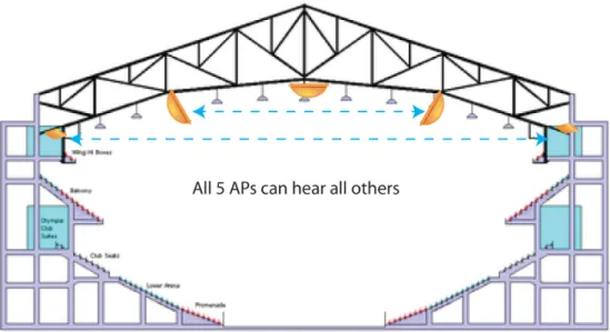
Venues such as stadiums have a higher likelihood of experiencing Wi-‐Fi interference. This is because these venues have a lot of open space, which also happens to be where the majority of attendees are located. When APs that have Line of Sight (LoS) to other APs (just as attendees can see one another in the stadium/arena), they will cause interference if they occupy the same channels.

(21)

Figure 1 -‐ Open spaces do little to restrict RF propagation

Most APs are installed in this space simply because this is where most devices are located. This means the likelihood some of APs will occupy the same channel is very high. The reuse factor can be calculated by dividing the total number of APs that can hear one another by the number of channels used. The higher this number in any given space the higher the self-‐interference experienced.

Exactly how much self-‐interference the Wi-‐Fi network generates depends on several factors such as the type of AP, antenna selection, where it is mounted, etc. The number of client devices will also fluctuate from one event to another based on attendance. The best rule of thumb is to keep potential interference as low as possible. This is the number one reason why deployments that over estimate the number of required APs see diminishing or even negative returns. Less is definitely more. The goal is to maximize capacity to the point where adding more APs no longer increases the aggregate capacity.

Non-‐Wi-‐Fi

While 802.11 interference will likely be the single largest source of RF interference, there are other sources. Non-‐Wi-‐Fi devices that use the same spectrum can cause problems. These devices commonly use the 2.4 GHz spectrum, although there are some that also use the 5 GHz range as well. Examples of this include microwaves, non-‐Wi-‐Fi cameras, cordless phones,

Zigbee wireless telemetry, headsets, frequency hopping microphones.

Non-‐802.11 RF interference can be difficult to diagnose since it is often generated at random times and is not always obvious. A site survey is always recommended for any Wi-‐Fi deployment before installation. This can be as elaborate as a formal survey or as simple as a quick tour of the building during business hours with an inexpensive RF analyzer such as the Wi-‐Spy 2.4x from MetaGeek, Fluke (AirMagnet) Spectrum XT, or a portable spectrum analyzer, such as those from Agilent or Antritsu.

(22)

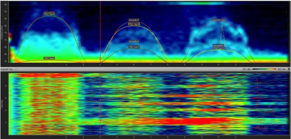
Figure 2 -‐ Wi-‐Spy recording of a lightly used Wi-‐Fi network on channel 11

Figure 3 -‐ A Wi-‐Fi network on channels 1, 6 and 11 with very heavy non-‐802.11 interference. This network is unusable.

(23)

Guidelines for Performance

As a general rule, the following will hold true for most very high-‐density Wi-‐Fi installations: • As density goes up, the amount of airtime dedicated to management traffic (scanning

for APs, broadcasts, etc.) will go up. This is also true as the number

of SSIDs broadcast increases. Both decrease the amount of airtime available for applications

• Avoid or reduce co-‐channel interference as much as possible

• Consider mounting APs in non-‐Line of Sight (NLoS) locations -‐ this will help attenuate the signal, which reduces the cell size and potential for co-‐channel interference. High-‐density applications have more than enough APs to make individual coverage a non-‐issue

• Make sure there are no other sources of RF interference nearby (non-‐802.11 sources)

• The more dense the population of devices, the higher the average latency and jitter -‐ this can limit the types of applications that can be supported in the most dense situations

• The goal for capacity is to maximize the SNR per AP

(24)

Estimating Client and AP Counts

The previous section discussed determining minimum performance requirements and factors that can affect the final deployments ability to deliver them. Without this information the rest of this document is as helpful since it cannot be tuned to correct parameters. This section

discusses the next step which is how many APs will be required for the design.

How many clients can I connect to a single AP?

This is the most common question asked about Wi-‐Fi. The answer changes dramatically depending on:

• Key performance metrics (applications, bandwidth, latency) • Client capability

• Estimated number of devices per AP • Physical density of people

• AP hardware selection

• Whether encryption will be utilized and what type

As discussed in the previous chapter, the minimum bandwidth and latency requirements for a device heavily influences how many clients an AP can support. This number in turn is used to calculate the amount of APs needed to satisfy the requirements.

Estimating the Number of Client Devices

While it is obvious all that all 20,000 attendees at a stadium will not use the network simultaneously, we still need to determine some reasonable number for network sizing. The state of a Wi-‐Fi device becomes an important factor i.e. if it is active and transmitting or associated but idle. Correctly scaling capacity needs to consider both the number of clients that might be connected as well as the number actually using the network. There should always be enough APs such that any random client can associate at any time and transmit data from any part of the coverage area.

(25)

Stadium Example:

The chance of all 20,000 attendees bringing a Wi-‐Fi device, connecting it and transmitting at the same time is almost nil; but there is no easy way to determine what number is likely. This is further complicated by the assumption the number of devices will increase over time. One way to estimate this number makes the following assumptions:

• The maximum number of Wi-‐Fi devices associated but idle on the network will always be greater than the number that are active

• Attendees will typically use one wireless device at a time

• Not all attendees will bring Wi-‐Fi devices or connect them to the network -‐ estimate 70%

• Unless otherwise indicated, no more than 80% of these devices are connected to the network

• Unless otherwise indicated, no more than 30% of all devices that are connected to Wi-‐Fi are active at the same time

Assuming an event at full capacity, some reasonable numbers to start with might look like this (see Table 4):

Percentage of

Uptake Number of Clients

Maximum capacity 100% 20,000

Attendees bringing a Wi-‐Fi device 70% 14,000

Devices connected to the WLAN 80% 11,200

Active devices 30% 3,360

Table 4

The percentages offered here represent a place to start3_{. If an existing wireless network exists,} it may have valuable information about the current number of active devices. If this is the case, the percentages should be adjusted accordingly.

There are several factors used to determine AP counts; • Association limit

• Capacity limit • Coverage limit4

3_{These percentages are based on actual observations during a sporting event in a sold-‐out stadium. The observed}

percentages were much lower (about half) of the guidelines offered here. This number was doubled to account for future smartphone growth and Wi-‐Fi enabled device usage.

(26)

Estimating the Access Point Association Limit

Ruckus APs currently support a maximum of 512 clients per AP. Therefore, the total number of APs needed to ensure all the Wi-‐Fi devices can get service if desired is calculated as follows:

Maximum number of Wi-‐Fi devices / 512 associations per AP

Estimating Access Point Throughput

The estimated aggregate throughput for an AP can be calculated as follows:

Maximum PHY rate * % of Overhead – Loss from interference (%)

As discussed earlier, TCP/IP networks often have as much as 40% overhead. This is subtracted from the raw available throughput to yield a clean RF number. However, high-‐density venues will see this number reduced due to collisions. This number is hard to pin down, but for these examples 35% is a reasonable place to start.

Stadium Example

The average expected throughput for an AP radio in the reference stadium is:

72.2 Mbps – (72.2 Mbps* .40 %) = 43.3 Mbps – (43.3 Mbps *.35) = 28.12 Mbps5

These numbers shown above are per radio. The lower number (2.4 GHz) is specifically called out here. 5 GHz radios should expect a slightly higher number.

When many APs are able to influence one another, such as in a very high-‐density deployment, the noise floor will rise. The same type of increase comes from the higher number of end user devices. The result is not all the user devices are able to achieve the highest modulation rate due to the noise floor increase and/or they are further away from the AP than the others. The resulting AP capacity will be a function of the blended rates of each end user devices

modulation rate resulting in the weighted average.

43.36_{Mbps – (43.3 Mbps* .40 %) = 26 Mbps – (26 Mbps *.35) = 16.9 Mbps}

This average is per radio, so a dual-‐radio AP could be expected to deliver twice this amount across two radios. However, since the second radio is 5 GHz and less subject to interference, it should deliver a higher number.

4_{Coverage limits are typically not an issue in very dense deployments and will not be discussed further.} 5_{This number is for 2.4 GHz radios – a 5 GHz radio should be higher}

(27)

Estimating Clients per AP Capacity

The maximum number of client devices a single AP can support with the required KPIs is then calculated as:

AP aggregate throughput / Minimum bandwidth per client

With the information so far, the maximum capacity for the example is:

Number of associated clients = 11,200

Estimated number of concurrent active devices = 30% of 11,200 = 3,360 Required throughput per client = 500 Kbps

Latency tolerance = high

RF environment = very high during peak usage

Percentage of retransmissions/loss due to interference = 35% Estimated throughput per AP radio = 16.7 Mbps

These figures are then calculated:

Maximum clients per AP to meet capacity = 33 (16.7Mbps / 500Kbps per client) Number of APs required to meet number of active clients = 102 APs (3360 / 33) Total APs for 11,200 associated devices = 22 (11,200 / 512)

Seats covered per AP = 196 (20,000 / 102)

The largest calculated number of APs, either for capacity or associations, is what is required to meet the service requirement.

Using these guides, 102 APs is the required number assuming the client devices are distributed evenly across all APs. However this is not a guarantee – some venues changing seating areas based on event type. It is always a good idea to allow for additional APs to cover this eventuality.

The only way to accurately estimate the weighted average capacity per AP is to do a computer simulation of the venue and calculate the SNR of each AP and the entire service area. Just estimating and using the peak value will yield to few APs and underestimating the per AP capacity will drive the AP count higher, which will in turn further reduce the weighted average per AP capacity.

Most venues will also require additional APs to cover areas outside the main stage. Coverage for concourses, ticketing areas, media areas offices, coaching, player ready area and backstage staging areas will increase the AP count. The exact number should be determined through an on-‐site survey and computer coverage simulation that accounts for exact construction and square footage.

(28)

Estimating Additional APs

Determining how many extra APs are required beyond the minimum count requires additional information:

• Distance from AP to client • AP cell (coverage) size

• Additional coverage areas outside the main bowl/stage

Because venues such as stadiums are very large and very dense, APs should ideally have small coverage areas. This increases performance and allows for narrower beam antennas that can boost signal gain. More APs also increases the receive signal for clients since there are more APs closer to any client location. This has the benefit of better SNR, which is required for high performance and capacity.

The directional antenna requirement is driven by the need for higher signal gain due to higher installation locations. They also help reduce interference. For more information on AP mounting strategies, please see section AP Installation and Hardware.

Distance from AP to Client

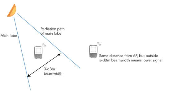
In general, an AP should be mounted as close to the clients as possible. RF signal strength is calculated as the inverse square of distance so the signal degrades quickly as distance increases. A client that is 30 meters (98 feet) from an AP receives a signal that is only 1/4th_{that (-‐6dB) of} a client 15 meters distant. A large enough distance can reduce the signal strength to the point where a client cannot hear it. This is particularly true if there is any background interference or noise.

(29)

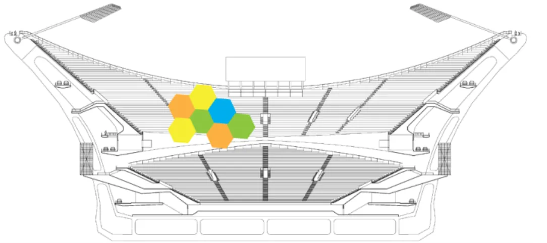
© 2012 Ruckus Wireless, Inc Best Practices v1.0 Using this model of AP positioning based on its beam width helps determine the coverage area for each AP. The need to get the APs closer is required to keep the AP foot print from being too large. It can help to think of each AP supporting a particular spot or section of seats within the stadium itself. Each additional AP adds another group of seats until all are covered.

Figure 5 -‐ Each region is the 3-‐dBm beam width coverage of an AP

Some venues will not necessarily have a structure in every location to support ideal AP installation. Open roof stadiums or outdoor sports fields are particularly challenging for this reason. In these cases compromises such as additional APs located at less than ideal spots may be required.

Guidelines for Estimating Capacity

Determining the number of APs required for a design can be complex. There are many variables that can come into play. As a general rule, the following rules of thumb will almost always apply:

• Plan for an adoption rate of about 50%-‐60% and 15% concurrent users • Estimate realistic AP goodput capacity that takes IP and 802.11 overhead

into consideration

• Do a RF SNR plan to estimate the interference and impact on the AP capacity • Ensure the number of clients per radio leaves some headroom (i.e. don’t plan the