THREE-STEP FIXED-POINT SKIPPING TECHNIQUE FOR UNCONSTRAINED NON-LINEAR MINIMIZATION PROBLEMS

InternatIonal Journal of ComputatIonal analysIs

Vol (3), No. (1), pp.

DOI: 10.33959/cuijca.v3i1.12

THREE-STEP FIXED-POINT SKIPPING TECHNIQUE FOR UNCONSTRAINED

NON-LINEAR MINIMIZATION PROBLEMS

Nudrat Aamir, Tazkia Anwar, Ayesha Nawaz, Aneesa Zeb, Lubna Zeb

Department of Electrical Engineering, City University of Science and Information Technology, Peshawar

Keywords:

Hessian

Lagrangian polynomial

A B S T R A C T

Ford and Moghrabi [2] introduced the multi-step quasi-Newton method for optimization, Where Hessian matrix is updated for each iteration, which outperformed the single step method. Jhon and Nudrat [4] introduced a multi-step skipping technique with and without modified search direction,, which shows a better experimental results. In Ford and Moghrabi, papers series, they introduced some techniques (Accumulative and Fixed-point approaches) to describe the parametric values needed to figure out the distances between many sets of iterations being involved in the recent interpolation curve. In this paper, we extended the existing three-step Fixed-point skipping approach and examine the sensitivity of this technique. Evidently, experimental result provides, positive improvement with comparison to standard Broyden-Fletcher-Goldfrab-Shanno (BFGS) method. Result shows comparatively, three-step Fixed-point n/4 skipping technique computational saves time than existing single-step BFGS method.

1. Introduction

Ford and Mograbi introduced multi-step quasi-newton methods for optimization, where current approximate Hessian is updated by utilizing data from more than one step. Where they present the idea, that employing interpolating curves, we can construct such methods. The standard quasi-newton method is also used in these methods, but in secant equation new vectors (r, w) are utilize instead of the normally used vectors (s, y). Where the quasi-Newton condition is defined as:

끀ᤧ (1)

(where the Hessian approximation 끀ᤧis needed to fulfill the above condition), is replaced by a similar condition,

끀ᤧ , (2)

where the vectors and are derived from the multi-step method under discussion.

In single-step quasi-Newton methods, the new approximation _끀ᤧ in single-step quasi-Newton methods, is essentially required to fulfill the requirement of quasi-Newton equation eq (1), which is an appropriate estimation to the equation of Newton method [1], [3]:

42

끀ᤧ h th h , (3)

Where the relation defined in above equation eq (3) is a clearly straight forward utilization of the Chain Rule application for the vector function th h : Where

h is restricted to satisfy 끀ᤧ and is defined to be any differentiable curve (indicate by X) in : the quasi-Newton equation eq(1) can be derived from

the Newton equation eq (3). If ( h ) is assumed to be defined by,

끀 (4)

From eq(4), we get,

ᤧ 끀ᤧ

And h , ,

Using interpolatory linear polynomial, we can estimate the curveth h such that,

t 끀 t ᤧ t

thenth h the derivative ofth h at ᤧ can be approximated by t ᤧ

t ᤧ t

t 끀ᤧ th ,

thus eq (3), becomes

끀ᤧ (5)

The approximation _끀ᤧto the Hessian h 끀ᤧ In the standard quasi-Newton method, is expected to fulfill the relation defined in eq(5) as an equality:

끀ᤧ (6)

Now we briefly discuss the concept of multi-step quasi-Newton methods ( ᤧ , in which the information is used from the most frequently utilized steps, where

the path is defined as the polynomial h of degree m interpolating the known point

끀 끀ᤧ t ᤧ (7)

Ford [2] found, that it is more comfortable to use the Lagrangian form of the interpolating curve

h 끀ᤧ (8)

where h presenting the Lagrangian polynomial of degree and is defined as

h (9)

If the gradient t is prescribed to the interpolating curve then by the comparatively interpolatory polynomial, it can be approximate

th h h th 끀 끀ᤧ (10)

In order to execute the Newton equation eq (3) with , we use the relation defined in eq (7) to find th h and eq (9) to guess th h :

By these values in eq (3) we then found the condition defined in eq (1) expected to be fulfill by the new Hessian approximation 끀ᤧ, where

h

h 끀ᤧ

(11)

th h _{h th}

끀 끀ᤧ

h ᤧ _{h (13)}

ᤧ_h ᤧ ₍₁₄₎

If we clarify eq (12) and eq (13) we can substitute and in charge of the most fresh employed step vectors ᤧ _and ᤧ_:

ᤧ ₍₁₅₎

ᤧ ₍₁₆₎

The new Hessian approximation 끀ᤧ, in multi-step procedure can be derived by utilizing any BFGS formula [2], where the vectors and are recouped by and , consequently:

끀ᤧ 끀 . (17)

correspondingly, to update the reverse Hessian approximation the BFGS-type method is given by

끀ᤧ 끀 ᤧ 끀 h 끀 (18)

and from the updated inverse Hessian approximation 끀ᤧwill be expected to fulfill the following condition

(19) The updating conditions for two-step and three-step methods are given as:

2. Multi-step methods 2.1. Two-Step

h 끀ᤧ ᤧ , (20)

h 끀ᤧ ᤧ , (21)

Where,

h ᤧ

hᤧ .

2.2 Three-Step

끀 ᤧh 끀ᤧ

ᤧ ᤧ 끀ᤧ끀 끀 ᤧ ᤧ끀

ᤧ

ᤧ 끀ᤧ끀 (22)

끀 ᤧh 끀ᤧ

ᤧ ᤧ 끀ᤧ끀 끀 ᤧ ᤧ끀

ᤧ

ᤧ 끀 ᤧ끀 (23)

끀ᤧ Where,

ᤧ h_hᤧ ᤧ and h_h

3. Unit-Spaced Method

We can determine (without failure of generality) the values as and _ᤧ ᤧ in single-step methodsh ᤧ : From correlation, in multi-step methods, the simplest preferred choice for the needed values of is a unit-spacing between the –values

끀 ᤧ t ᤧ h (24)

From eq (21) and eq (22) the vectors and are presented as,

, , _끀ᤧ .

44

In this method, where , the data utilizes from the current last three iterates _{ᤧ 끀ᤧ} and analogous gradient values. The values of are given as:

ᤧ ᤧ ᤧ = 1 and, from eq (19) and eq (20), the values of vectors and are given by ᤧ

ᤧ ᤧ ᤧ, 끀ᤧ

3.2. Unit-spaced Three-step Method

In this method, , and the information of data used is obtained from latest four iterates ᤧ 끀ᤧ and their interrelated gradient values. The values of

ᤧ ᤧ ᤧ

Taking the values of ᤧ and ᤧ, then we have from the relation defined in eq (21) and eq (23), the values of vectors and are given by

ᤧᤧ ᤧ끀ᤧᤧ , ᤧᤧ ᤧ끀ᤧᤧ 끀ᤧ

4. Metric based approaches

In metric-based approaches the values of are derived by measuring the distances between the mostly fresh recent iterates 끀 끀ᤧ . To figure out the distances between iterates 끀 끀ᤧ , through metric based procedure the matric

is used. For example, to calculate the distance between iterates 끀ᤧand we calculate

끀ᤧ 끀ᤧ 끀ᤧ

ᤧ

h ᤧ

where is a positive-definite matrix. Some of the choices considered for are as follows.

4.1. The Identity Matrix

The most simplest choice matrix for M is the identity matrix. Therefore, we can figure out the distance among the points and ᤧby

ᤧ ᤧ ᤧ

ᤧ ᤧ

4.2. The Current Hessian Approximation

The choice look like a natural one. In this case,

ᤧ h ᤧ h ᤧ

ᤧ

h ᤧ

5. The Fixed-Point Methods

In Fixed-point methods the metric is used to figure out the distance of every single iterative point from one particular selected iterate (consider as the fixed point, which thereby becomes the origin for values of ). In this approach, the latest iterate 끀ᤧ is taken to be the fixed-point giving, ( ) and we then compute the other parametric values by measuring precisely the distance between 끀 끀ᤧand 끀ᤧ:

끀ᤧ 끀 끀ᤧ t ᤧ

Now, we will examine Three-step methods of fixed-point approach:

To figure out the values of τ , we fix one of the iterative point as origin say _끀ᤧ, This iterative point corresponds to so we consider as origin, such that , and calculate the values of , ᤧand by measuring the distance from 끀ᤧ to and

ᤧ directly. Distance is measured by using the above defined metric.

ᤧ h ᤧ h ᤧ

ᤧ

Now consider algorithms for and (where is a single step implicit update of ). First we define some relations which will be used in the algorithms defined below.

We know that

ᤧ ᤧ ᤧ

and

, where,

ᤧ ᤧ_ᤧt ᤧ, ᤧ

ᤧ _{t , (because we skipped the update of} ᤧ). Therefore, we obtain

ᤧ ᤧ _{t .}

Using the above relations, we therefore find that

ᤧ t ,

and

ᤧ ᤧ ᤧt ᤧ

As we define above,

h _ᤧ

For

h We know that and

ᤧ _t which gives us

h _{t (5.1.1)}

Similarly (because of skipping) ᤧ

h

ᤧt ᤧ (5.1.2)

and

h _{t (5.1.3)}

We define 䁢 ꀀh ᤧ ᤧ which gives us h

46 ᤧ _ᤧ

ᤧ ᤧ 끀

ᤧ _ᤧ ᤧ ᤧ

h h ᤧh

ᤧ h ᤧ 끀

ᤧ _ᤧ

ᤧ ᤧ (5.1.4)

Using eq (5.1.1) and eq (5.1.2) also,

h

ᤧ ᤧ

ᤧ ᤧ 끀

ᤧ _ᤧ ᤧ ᤧ

h h ᤧ

ᤧ h ᤧ

끀 ᤧh ᤧ

ᤧ ᤧ (5.1.5)

utilizing eq (5.1.2) and eq (5.1.3) also,

ᤧ h

ᤧ

ᤧ (5.1.6)

Now, we discuss Fixed-point Algorithms.

5.1.1 Algorithm

For , let us consider, Then,

h 끀ᤧ ,

also,

ᤧ h 끀ᤧ ,

끀 ᤧ , and

h 끀ᤧ ,

끀 ᤧ끀 .

5.1.2. Algorithm

Taking we have, Then,

h 끀ᤧ using eq (7.1.5).

Also,

Using eq (7.1.5) and eq (7.1.6). Now finally we calculate,

h 끀ᤧ 끀 ᤧ끀 h 끀 ᤧ끀 끀 ᤧ끀 ᤧ ᤧ끀

끀 _ᤧ h 끀 h

From eq(7.1.4), eq (7.1.5) and eq (7.1.6).

6. Numerical results

The proposed idea in this paper is tested on existing single step, existing unite-spaced and on existing Three-step fixed point method and then the Three-step fixed point method with the skipping and is compared with single step and unite spaced BFGS method. All the algorithms in the experiments will utilize the BFGS formula in computation to update the inverse Hessian approximation

ᤧ

But (in the case of multi-step methods) with the usual vectors and replaced by and :

끀ᤧ ᤧ끀 ᤧ 끀 h 끀

Total 25 test functions are tested in the experiments with different dimensions rang start from 2 to 200. These were selected from standard problems expressed in the literature [5]. Four distinct starting points were employed, for each function, which gives a total of 100 test problems. All these test functions were classified into the following different subsets (where n is the dimension of the vector x):

(1) Low : (2 ); (2) Medium : (21 ); (3) High : (61 ); (4) Combined : (2 ).

According to classification in total their are 3, 7 and 15 problems in low, Medium and high respectively. Therefore, in each subset their are 12, 28 and 60 test problems located respectively. All these functions are selected from J.J. Mor, B.S. Garbow and K.E. Hillstrom [5] and Toint [6].

Table 6.1. Problems and dimensions Problems Dimension

Extended Rosenbrock 2, 20, 26, 40, 60, 80, 100, 120 Merged Quadratic [6] 30, 50, 70, 110, 136, 180 Discrete integral equation 20, 84, 100, 150, 175, 200 Freudenstein and Roth [6] 28, 52, 85, 118, 190

In this paper we have discussed existing standard BFGS method and quasi-newton methods. The proposed idea, skipping updates was implemented on BFGS and three-step fixed-point technique. The proposed idea were tested on four different functions with dimensions ranging from 2 to 200, as discussed in table ( Table 6.1.).

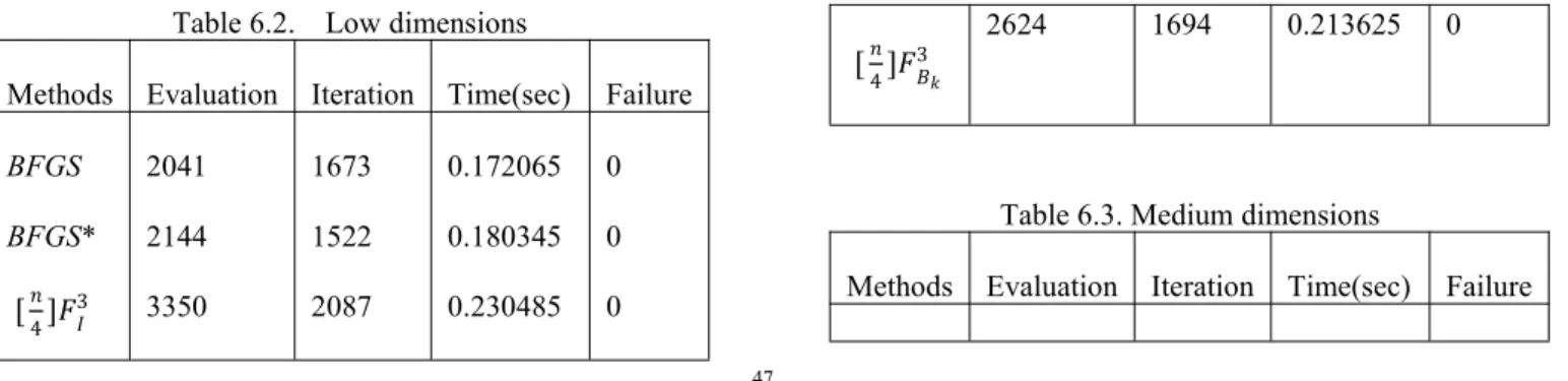
In this section the experimental results of three-step skipping technique and the non-skipping single-step BFGS methods for 'low', 'medium' and 'high' dimensions are discussed. Experimental results were obtained from MATlAB R2009b and Windows7 in Shaheed Benazir Bhutto Women University Peshawar lab. All the skipping techniques are discussed in comparison with single-step BFGS methods.

Table 6.2. Low dimensions

Methods Evaluation Iteration Time(sec) Failure

BFGS BFGS*

䁢

2041 2144 3350

1673 1522 2087

0.172065 0.180345 0.230485

0 0 0

䁢 2624 1694 0.213625 0

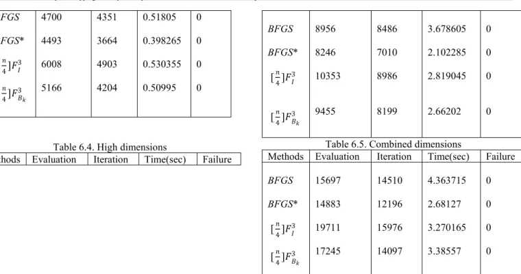
Table 6.3. Medium dimensions

48

BFGS BFGS*

䁢 䁢

4700 4493 6008 5166 4351 3664 4903 4204 0.51805 0.398265 0.530355 0.50995 0 0 0 0

Table 6.4. High dimensions

Methods Evaluation Iteration Time(sec) Failure

BFGS BFGS*

䁢

䁢

8956 8246 10353 9455 8486 7010 8986 8199 3.678605 2.102285 2.819045 2.66202 0 0 0 0 Table 6.5. Combined dimensions

Methods Evaluation Iteration Time(sec) Failure

BFGS BFGS*

䁢 䁢

15697 14883 19711 17245 14510 12196 15976 14097 4.363715 2.68127 3.270165 3.38557 0 0 0 0 Investigating the results, we have observed that BFGS* (single step method with n/4 skipping) performing much better in computational time saving, function evaluations and iterations for medium, high and combined dimensions . But for low dimensions the non-skipping single-step BFGS method shows progress on all skipping techniques BFGS*, 䁢h and 䁢h . Since we know that the solution for low and medium dimension is easy to implement. Therefore, in this thesis we are emphasize on high and combined dimensions. Observing results, we conclude that the skipping techniques BFGS*, 䁢 and 䁢 working much better than non-skipping BFGS method. Skipping techniques saves computational time than non-skipping BFGS method. But unfortunately, the number of iterations and evaluations are increasing in 䁢 and 䁢 .

7. Conclusion

In this paper we have investigated the standard BFGS method and three-step fixed-point technique with skipping idea i.e skipping updates. From above discussion we have concluded that the new skipping idea performs better than non-skipping idea in case of computational time, although the functions evaluations are increasing. We have also noticed that for low and medium dimensions single-step standard BFGS method outperform the three-step fixed-point techniques with proposed skipping idea. Since the solution for low and medium dimensions is easy to implement, therefore, in this paper we have focus on high and combined dimensions. Evidently, from results we have noticed that the skipping techniques succeeded in saving computational time for high and combined dimensions as compared to standard BFGS method.

R

[1]. J. A. Ford, “On the use of additional function evaluations in quasi-newton methods”, Department of Computer Science, University of Essex, 1986.

[2]. J. A. Ford and I. A. Moghrabi, “Multi-step quasi-newton methods for optimization”, Journal of Computational and Applied Mathematics, 1994.

[3]. J. A. Ford and A. F. Saadallah, “A rational function model for unconstrained optimization", Colloquia Mathematica Societatis Janos Bolyai, 1986.

[4]. J. A. Ford and N. Aamir, “Multi-step skipping methods for unconstrained optimization”, Numerical Analysis and Applied Mathematics Icnaam 2011.

[5]. J. J. Mor , B. S. Garbow and K. E. Hillstrom,” Testing unconstrained optimization software”, ACM Transactions on Mathematical Software, 1981.

[6]. Ph. L. Toint, “On large scale nonlinear least squares calculations”, SIAM Journal on Scientific and Statistical Computing, 1987), no. 3, 416-435.