Thesis

(1)

A Comprehensive Analysis of the Escalation of Commitment in Professional Basketball

By

Matthew McCauley

Honors Essay Economics

University of North Carolina

April 1, 2014

Approved:

(2)

Abstract

Traditional economic theory suggests that decision makers should not allow sunk costs to shape future actions. However, empirical studies have found a commensurate relationship

(3)

Acknowledgements

There are many people responsible for the success of this research. First and foremost, I would like to thank my advisor Dr. Rita Balaban for her support and guidance throughout the entire process. Beyond her role as my advisor, her instruction in Economics 101 sparked my interest in this discipline, and without that experience I would never have been given this

(4)

1

I. Introduction

Traditional economic theory suggests that decision makers should not allow sunk costs to shape future actions. To allow these costs to affect a decision is to commit the Sunk Cost

Fallacy, an irrational action that empirically is quite common. From politics to managerial choices to everyday economic decisions, evidence of this fallacy can be found throughout many disciplines (Staw, 1997; Garland, Sandefur and Rogers, 1990). In fact even US Presidents have succumbed to this Fallacy. Both Lyndon B. Johnson and George W. Bush openly justified military action through previously incurred monetary and human costs (Staw, 1997; Manier, 2006). Examining this fallacy, studies have found a commensurate relationship between sunk costs and future expenditures in a failing project, an idea known as the “escalation of

commitment” (Staw, 1976).

In professional sports, labor choices are among the most important managerial decisions (Késenne, 2007). With large sunk costs incurred through annual player drafts, executives in the high-stakes business of professional sports may be particularly prone to the escalation of commitment. Under the goals of maximizing wins and profits, the rational action would be to play the most productive and lucrative players. However, there is plenty of anecdotal evidence to suggest that this is not always the case. Every year disgruntled sports fans and expert

commentators are perplexed by the various personnel decisions made by their favorite teams.

(5)

2

individual’s draft position predicts playing time or retainment, NBA teams may be guilty of

escalation of commitment.

The previous studies on this topic have not fully encompassed the recent theoretical literature, have not been updated through the past four Collective Bargaining Agreements (CBAs) and have not utilized the most accurate performance measures. Recent theoretical research has shown that there is often rational behavior behind what is ostensibly the escalation of commitment. This study is conducted in light of this new theory, and the models are updated to appropriately separate rational behavior from what is perceived as irrational decision making. Also, as the current research in the literature has examined data only through the 1991 draft, this analysis better explains the dynamics of the present-day NBA. Lastly, instead of using the simple performance measures in the previous studies, the models in this paper utilize advanced statistics such as John Hollinger’s Player Efficiency Rating and the Win Shares metric.

In addition to multivariate analysis, this study also employs a logistic model. Though Staw and Hoang (1995) completed an event series analysis, a logistic model should allow assessments on a year-to-year basis while eliminating issues in the interpretation of a survival analysis. This study anticipates that a careful consideration of the newest theory, along with improved models and a vastly different NBA salary environment, will lead to finding less

(6)

3

II. Literature Review

A. Theoretical Background

The recognition of the Sunk Cost Fallacy and its relevance to decision-making is not a new phenomenon. Beginning with Kahneman and Tversky (1979), traditional utility theory was challenged in favor of Prospect Theory which sought to illustrate decision making under risk. To begin this discussion, consider traditional utility theory where is the utility of outcome and is the probability of its occurrence. The expected utility of a set of potential outcomes is

calculated as follows:

(1) ∑ .

Furthermore, a prospect is added to an asset class, w, when

(2) ∑ .

This equation shows that a prospect is considered when its expected utility is a net benefit.

Kahneman and Tversky (1979) found in many experiments that individuals undervalue possible opportunities and overvalue guarantees. Furthermore, individuals were risk loving with sure losses and risk averse with definite gains. These empirical findings can be incorporated into a value function. In this function, utility is replaced by value, , which is a change in wealth relative to an initial reference point. The likelihood of occurrence, , denotes an

(7)

4 (3) ∑ .

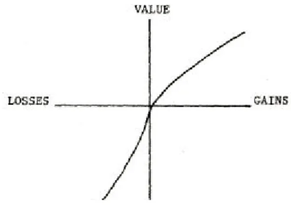
Thaler (1980) outlined this value function over a gains and losses plane according to general premises backed by both economic and psychological principles. The value function is steeper over losses than it is over gains. This reflects the psychological principle that any given magnitude of value provides more aggravation when lost than it does pleasure when gained. Furthermore, the function is concave over gains and convex over losses to incorporate risk-loving behavior with losses and risk-averseness with gains. This also implies that an identical difference between two values is perceived differently depending on their magnitude. For example, moving from 0 to 10 is greater value than from 500 to 510. This phenomenon has consistently been shown with experiments and even observed in large settings such as the US stock market (Weber and Camerer, 1997).

In the context of this study, this may explain why teams are prone to the escalation of commitment with higher draft picks. Consider a recently drafted player who is described as with representing value in the losses plane. Thus a player has potential value of and his salary and other costs are c. Only if his costs are greater than his gains is their “pain.” Consider a team that is indifferent to playing a “free” player, meaning . Then, if

a player incurs a salary, s, the value equation becomes ( ) Because of risk-loving behavior in the losses space, ( ) . Therefore, a team

(8)

5

Figure 1: Value function as defined by Thaler (1980)

As for empirical studies, Arkes and Blumer (1985) examined the Sunk Cost Fallacy through a series of psychological experiments that studied individuals’ decisions on events such as ski trips and movie theater showings. Overall they found that subjects were more likely to choose unsatisfying options with previously incurred costs over enjoyable alternatives with no incurred costs. Another experiment presented students with a managerial decision to invest in an incomplete project. In this study, they concluded a “greater tendency” to continue an endeavor

once invested.

Furthermore, Boehne and Paese (2000) conducted a comprehensive set of experiments that presented subjects with varying degrees of completion and a “sales price” of a completed project. Though they found that individuals acted more rational than they did in the previous studies, they confirmed a “completion effect” where the closer individuals were to completing a

project the more likely they were to continue with an endeavor (p. 178). In the NBA, if a young player is the “project,” teams may believe higher picks are closer to “completion,” or their

expected career performance levels which could lead to increased playing time.

(9)

6

they presented three general rational aspects to help explain the escalation of commitment. First, as sunk costs are correlated with future costs, they can shape expectations of future costs and reveal informational content of a project. This means that the aforementioned “completion effect” observed in previous studies actually can be rational.

To explain this, they present a simple two-period decision where and are the

incurred costs and probability of completion in time period i. The completion cost, ̅, is

unknown and distributed according to a cumulative distribution function, ̅ The cumulative

hazard of investment is

(4) .

Therefore, because depends on it is rational to consider previously incurred costs when

evaluating commitment in time period 2. Furthermore, with an increasing hazard rate in time period 1, the willingness to invest in time period 2 is positively related to sunk costs.

Second, under asymmetrical information, a manager may rationally continue a project in order to conceal that it was a failure and thus prevent reputation damages. In the NBA, after drafting a player higher than the general consensus expected, a team may play or keep a player to prevent its decision to appear wrong or ill-advised. Therefore, a change of a team’s coach or general manager (GM), who are often teams’ primary labor decision makers, may negatively affect a draft pick’s playing time. This study incorporates this theory by introducing a dummy

variable for a coach or team executive change. A player drafted high above his market value (i.e. higher than a third-party evaluation) may be played by a team to prevent from admitting it has made a mistake. In this sense, reputational “costs” manifest in decision makers’ stubbornness

(10)

7

Third, financial and time constraints can determine an individual’s ability to undertake another project. As an individual’s previous costs affect the ability to undertake a second option, budget constraints can cause an individual to continue with a current project. Empirically, Tan and Yates (2002) found that the prospect of overspending a budget actually deters the escalation of commitment. However, they also found that budgets can eschew the likelihood of undergoing beneficial investment opportunities. In the NBA, recent CBAs have reduced teams’

commitments to high picks while rookie contracts have become a smaller part of teams’ overall

payrolls (Hill and Jolly, 2012). However a team may play a rookie simply because it is the only available option given its budget constraints and the talent distribution in the league.

B. Professional Sports Labor Market

To fully evaluate the escalation of commitment, the study must consider and ultimately assume certain motives behind NBA decision making. Zimbalist (2003) asserts that NBA owners may not strictly obey a profit-maximizing philosophy on a year-to-year basis but rather seek to maximize global and long-term returns. Berri, Brook and Schmidt (2004) found that wins maximize ticket sales in the NBA, not star power. For the purpose of this study it is assumed teams are profit-maximizers that value wins as their primary revenue-generators. It has been noted that external factors such as player popularity could motivate teams to play certain players. Though Staw and Hoang (1995) considered that this may affect a player’s draft position and

subsequent playing time, they assumed that any leftover popularity from college would soon dissipate and thus quickly become irrelevant to playing time decisions. Camerer and Weber (1998) recognized the potential effects of player popularity but were ultimately unable to find a metric that quantified a player’s popularity. Since then Berri, Schmidt and Brook (2004) found

(11)

8

individual popularity may cause increased revenue, this research maintains that a player’s ability to “create” wins is paramount. For the ease of modeling, this study assumes that fans’ affinities

for certain players do not motivate playing decisions.

Furthermore, established sports economic theory suggests that the uncertainty of

outcomes drives popularity (Keohane and Shmanske, 2012). As professional basketball has long experienced the lowest competitive balance of the four major North American leagues, the NBA has an incentive to promote team equality (Vrooman, 1995). Used in every major North

American sports league, the reverse-order player draft is perhaps the most notable tool to increase competitive balance. Over the past 30 years, the league has instituted additional restrictions to increase its competitive balance, most notably a “soft” team salary cap in 1984.

Overall, however, NBA salaries were governed by a loose set of restrictions prior to the 1995 CBA (Hill and Jolly, 2012).

In 1995 the NBA and the Player’s Association instituted rookie scale contracts, providing

(12)

9

Hill and Groothius (2001) use the Median Voter Theorem to explain why individual salary caps were instituted in 1999. As top draft picks were often paid exorbitant amounts, this Theorem could be applied to explain why the Union initially approved of rookie scale contracts. Hill and Jolly (2012) attribute both the 1995 introduction of rookie contracts and the 1999 extension from three to four years to corresponding decreases in salary inequality. In particular, they found a significant economic rent shift from superstar rookies to veterans. Since rookies have become relatively cheaper and their associated sunk costs have become lesser in magnitude, theory predicts a decrease in escalation of commitment.

Given the draft’s importance to improvement, teams have clear incentives to draft the

best players and the ones most likely to produce wins. However, studies have concluded that professional sports teams are far from perfect at evaluating talent. Studying all major

professional sports, Koz, Fraser-Thomas, and Baker (2011) found that draft position is a significant predictor of playing time but not a great predictor of performance. In the National Football League (NFL), Berri and Simmons (2011) concluded that teams are not very good at predicting quarterback performance. On the contrary, Boulier, Stekler, Coburn, and Rankins (2010) found that NFL teams are relatively successful at evaluating the future success of quarterbacks.

(13)

10

aging led to a decline of six draft spots. For the sake of this study, it is important to understand that the market of NBA entrants may be inefficient. This inefficiency requires teams to re-evaluate their picks and continuously update their performance expectations, which provides the opportunity for escalation.

C. Previous Studies

Staw and Hoang (1995) conducted the initial research on the escalation of commitment in the NBA using data from the first five years of the players taken in the 1980-86 drafts. Using generic performance indexes and controlling for position, injury and trade, they found that draft position was a significant predictor of playing time in each of the first four years of players’ careers. In addition, through an event history analysis, they found that draft position was a highly significant predictor of career longevity.

Camerer and Weber (1998) modified Staw and Hoang’s models. First, to account for team environments they used backup player performance, instead of simply team winning

percentage. If a pick’s backup is unsatisfactory, then a team may have no other option but to play

the draft pick. Second, recognizing that draft position may provide inherent expectations of a player’s future productivity, they controlled with a third party pre-draft ranking. Third, to

(14)

11

prior escalation. Lastly, in addition to lagged performance variables, they also used

contemporaneous and decomposed performance indices. Contrary to their hypothesis, evidence of escalation persisted. In fact, they found draft position to be a significant predictor through the first three years, only one year less than discovered by Staw and Hoang.

D. Advanced Performance Metrics

Both of these studies used three-category performance indices: “scoring”, “toughness” and “quickness.” From a basketball perspective, the comprehensive statistics employed in this

study are well-regarded tools to evaluate performance. The first statistic used in this study is John Hollinger’s Player Efficiency Rating (PER). Using linear weights, this statistic utilizes the entire box score to evaluate a player’s ability on a per minute basis. Though PER incorporates

positive and negative characteristics and controls for game environment, Berri and Bradbury (2010) note that it is not highly correlated with wins. Therefore this study also considers a second metric, the Win Shares statistic (WS). This metric measures a player’s marginal win product. Using both team and individual performance, the WS statistic computes a player’s

(15)

12

III. Econometric Model

In their study, Staw and Hoang (1995) proposed a simple multivariate model to estimate minutes played per season on a year-to-year basis (t= time in years). However, to account for the 2011 shortened season, the dependent variable was switched to minutes played per game. This model was employed to compare the data between the studies:

(5)

Min= minutes played per game

S= Scoring

T= Toughness

Q= Quickness

Inj= injury

Tr= trade

Win= team winning percentage

D= draft number

Pos= guard or forward/center

Camerer and Weber (1999) modified this regression:

(6)

X= vector of variables used in Model (1)

BS, BT, BQ= back-up player performance indices

B= belief, or third-party pre-draft evaluation of player’s ability

(16)

13

In this study, the multivariate model is based off equation (6) and equation (7):

(7)

P= vector of lagged and contemporaneous performance measures (PER/WS)

T= vector of team performance measures (win percentage, offensive efficiency and defensive efficiency)

I= injury

C= head coach or general manager firing

B= third-party pre-draft evaluation

In this model a dummy variable for a head coach or general manager firing is included to address a potential reputational concern. If the predictive value of draft position diminishes after a coach or GM change then reputational “costs” could have motivated a player’s playing time or

survival on a team.

Though Staw and Hoang (1995) used an event history analysis, such an analysis is invalid. A fundamental assumption of this study is that draft pick is a proxy for a player’s salary. As ensuing contracts are not necessarily related to draft position, this assumption is invalidated once the initial contract expires or is terminated. Even more troublesome, the same expectations that motivated a player’s initial draft position may rationally motivate an ensuing contract given

that the contracts, i.e. sunk costs, are indeterminate and may incur little commitment. Therefore, analyzing the effect of pick on survival can be misleading.

Instead of an event history analysis a logistic regression is used to analyze decision making on a year-to-year basis. Also, with consideration of the relevant CBA, this model evaluates how rookie scale contracts affect a team’s decision to retain a player. The model is as

(17)

14 (8)

Ret= whether a team elects to retain a player

Z= vector of player and team factors in Model 3 without Injury and Trade

Considering the aforementioned lockstep relationship between pick and salary for first round picks, Models (7) and (8) will consider both a sample limited to first round picks and a pooled sample. Furthermore, the first round sample will be separated by CBA to determine if the change in rookie contracts affected teams’ behavior. Lastly, draft position will be removed from the equation to evaluate the sole effect of round. Though there is a lockstep salary structure for first round picks, the differences in amounts are not only relatively minor but exempt from the salary cap. Thus all first round picks may effectively incur equal commitment to teams. Therefore, pick is removed from the model to evaluate round’s sole effect on retainment.

IV. Data

All of the individual and team data were obtained from www.basketball-reference.com with the exception of injury data which were extracted from www.prosportstransactions.com. The data consist of all players from the 1999-2008 draft classes. Variable definitions and descriptive statistics are available in Appendix B.

V. Results & Discussion

(18)

15

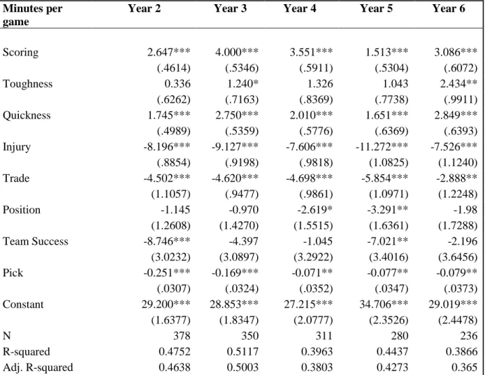
quite similar to those found by Staw and Hoang. With R-squared values between .39 and .51, this model proved to be a slightly better fit than with Staw and Hoang whose R-squared values never exceeded .46.

Table 1: Staw and Hoang model with Performance Indexes1

Note: *** denotes p-value<.01;** <.05; and * <.1. Standard errors are in parentheses and trade is a two-side test.

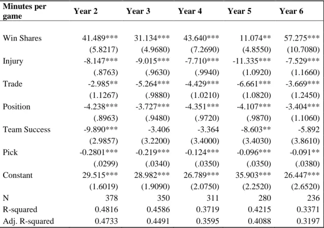
As seen in Table 2, when the performance indexes were replaced with the advanced metric Win Shares, the model performed slightly worse. Compared to the Table 1 results, pick was greater in magnitude and was more significant in the later years. Injury, trade and team

1

The regressions begin with Year 2 because of the lagged performance variable. Also, as the 2013-2014 season marks the sixth year for the 2008 class, these players were excluded from all of the Year 6 regressions.

Minutes per game

Year 2 Year 3 Year 4 Year 5 Year 6

Scoring 2.647*** 4.000*** 3.551*** 1.513*** 3.086***

(.4614) (.5346) (.5911) (.5304) (.6072)

Toughness 0.336 1.240* 1.326 1.043 2.434**

(.6262) (.7163) (.8369) (.7738) (.9911)

Quickness 1.745*** 2.750*** 2.010*** 1.651*** 2.849***

(.4989) (.5359) (.5776) (.6369) (.6393)

Injury -8.196*** -9.127*** -7.606*** -11.272*** -7.526***

(.8854) (.9198) (.9818) (1.0825) (1.1240)

Trade -4.502*** -4.620*** -4.698*** -5.854*** -2.888**

(1.1057) (.9477) (.9861) (1.0971) (1.2248)

Position -1.145 -0.970 -2.619* -3.291** -1.98

(1.2608) (1.4270) (1.5515) (1.6361) (1.7288)

Team Success -8.746*** -4.397 -1.045 -7.021** -2.196

(3.0232) (3.0897) (3.2922) (3.4016) (3.6456)

Pick -0.251*** -0.169*** -0.071** -0.077** -0.079**

(.0307) (.0324) (.0352) (.0347) (.0373)

Constant 29.200*** 28.853*** 27.215*** 34.706*** 29.019***

(1.6377) (1.8347) (2.0777) (2.3526) (2.4478)

N 378 350 311 280 236

R-squared 0.4752 0.5117 0.3963 0.4437 0.3866

(19)

16

success had similar effects. Interestingly, unlike the initial model, position had a highly significant negative coefficient, suggesting that guards experienced more playing time. In the initial model toughness accounted for forward/center qualities (rebounds and blocks) and

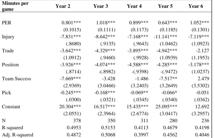
quickness consisted of guard statistics (assists and steals). These performance indexes could have absorbed the explanatory power provided by position in the Win Shares model. As seen in Table 3, when the linear-weighted PER metric was used, pick was highly significant through Year 3, and was significant at the 5% level in Year 4.

Table 2: Staw and Hoang model with Win Shares Minutes per

game Year 2 Year 3 Year 4 Year 5 Year 6

Win Shares 41.489*** 31.134*** 43.640*** 11.074** 57.275***

(5.8217) (4.9680) (7.2690) (4.8550) (10.7080)

Injury -8.147*** -9.015*** -7.710*** -11.335*** -7.529***

(.8763) (.9630) (.9940) (1.0920) (1.1660)

Trade -2.985** -5.264*** -4.429*** -6.661*** -3.669***

(1.1267) (.9880) (1.0210) (1.0820) (1.2450)

Position -4.238*** -3.727*** -4.351*** -4.107*** -3.404***

(.8963) (.9480) (.9720) (.9870) (1.1060)

Team Success -9.890*** -3.406 -3.364 -8.603** -5.892

(2.9857) (3.2200) (3.4000) (3.4030) (3.8610)

Pick -0.2801*** -0.219*** -0.124*** -0.096*** -0.091**

(.0299) (.0340) (.0350) (.0350) (.0380)

Constant 29.515*** 28.982*** 26.789*** 35.903*** 26.447***

(1.6019) (1.9090) (2.0750) (2.2520) (2.6520)

N 378 350 311 280 236

R-squared 0.4816 0.4586 0.3719 0.4215 0.3371

Adj. R-squared 0.4733 0.4491 0.3595 0.4088 0.3197

Altogether, substituting advanced performance metrics into the Staw and Hoang model did not drastically change the results. The results from the PER model deviated from the

(20)

17

significant through Year 5. Moreover, the adjusted R-squared values were consistently higher for the PER model. To limit redundancy in the other models, PER was the only performance statistic used going forward.

Table 3: Staw and Hoang model with PER Minutes per

PER 0.801*** 1.018*** 0.899*** 0.643*** 1.052***

(0.1015) (0.1111) (0.1173) (0.1185) (0.1301)

Injury -7.831*** -8.642*** -7.168*** -11.141*** -7.119***

(.8680) (.9135) (.9643) (1.0462) (1.0923)

Trade -3.642*** -4.329*** -3.895*** -4.942*** -2.127

(1.0912) (.9460) (.9928) (1.0939) (1.1953)

Position -3.926*** -4.074*** -4.588*** -4.285*** -3.178***

(.8714) -(.8982) -(.9398) -(.9472) (1.0237)

Team Success -7.669*** -3.428 -1.486 -7.517** 2.479

(2.9369) (3.0466) (3.2403) (3.2649) (3.5302)

Pick -0.245*** -0.168*** -0.069** -0.066* -0.051

(.0300) (.0321) (.0345) (.0340) (.0362)

Constant 20.304*** 16.517*** 15.435*** 25.095*** 12.692

(2.0551) (2.3964) (2.6774) (3.0417) (3.2957)

N 378 350 311 280 236

R-squared 0.4953 0.5153 0.4113 0.4679 0.4198

Adj. R-squared 0.4872 0.5068 0.3997 0.4562 0.4046

(21)

18

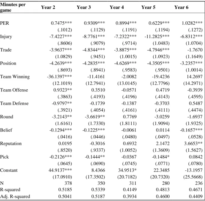
and round were irrelevant. Given that their sample was prior to the institution of the Rookie Scale contract, round may have become important once first round picks were mandated guaranteed money. The reputation coefficient was positively significant in Year 6 and insignificant in all other years. The positive relationship, which suggests that a coach or

executive change increases playing time, was contrary to expectations. Compared to the previous model, the adjusted R-squared values were higher in all years, except in Year 4 when it was slightly lower.

(22)

19

Table 4: Modified model controlling for reputation concerns, informational content and first-round guaranteed money Minutes per

PER 0.7475*** 0.9309*** 0.8994*** 0.6229*** 1.0282***

(.1012) (.1129) (.1191) (.1194) (.1272)

Injury -7.4227*** -8.7761*** -7.2322*** -11.2825*** -6.8312***

(.8606) (.9079) (.9714) (1.0483) (1.0704)

Trade -3.9637*** -4.8344*** -3.8875*** -4.7946*** -1.7670

(1.0829) (.9451) (1.0015) (1.0923) (1.1649)

Position -4.2639*** -4.2835*** -4.6269*** -4.3505*** -3.2357***

(.8693) (.8941) (.9583) (.9501) (1.0014)

Team Winning -36.1397*** -11.4161 -2.0082 -19.4236 14.2697

(12.1019) (12.7941) (13.0145) (12.7796) (14.2971)

Team Offense 0.9323** 0.3510 -0.0571 0.4719 -0.3939

(.3863) (.4193) (.4196) (.4143) (.4595)

Team Defense -0.9797** -0.1739 -0.1387 -0.3703 0.5487

(.3921) (.4054) (.4161) (.4111) (.4474)

Round -3.2143** -3.6619** 0.7769 -3.0259 -1.6937

(1.6161) (1.7330) (1.8111) (1.9094) (1.9325)

Belief -0.1294*** -0.1225*** -0.0061 0.0114 -0.1657***

(.0416) (.0446) (.0480) (.0497) (.0528)

Reputation 0.0195 -0.3016 0.6932 2.1472 3.6653**

(.8520) (.9337) (1.0052) (1.3609) (1.5627)

Pick -0.2126*** -0.1444** -0.0367 -0.1484* 0.0842

(.0645) (.0690) (.0745) (.0771) (.0780)

Constant 44.9137*** 8.4366 34.9513* 22.3485 -13.1957

(17.0910) (17.3502) (20.7182) (20.7320) (25.5668)

N 378 350 311 280 236

R-squared 0.5185 0.5339 0.4149 0.4813 0.4671

Adj. R-squared 0.5041 0.5187 0.3934 0.4600 0.4409

(23)

20

Table 5: Modified model with lagged and contemporaneous performance Minutes

per game Year 1 Year 2 Year 3 Year 4 Year 5 Year 6

PER Year 1 0.6703*** 0.4897*** 0.1621 0.0169 0.3554** 0.2075

(.0775) (.1049) (.1245) (.1478) (.1532) (.1586)

PER Year 2 0.5725*** 0.2271* 0.1885 -0.0194 0.1086

(.0920) (.1251) (.1739) (.1863) (.2066)

PER Year 3 1.0637*** 0.244 0.0379 -0.077

(.1118) (.1726) (.1961) (.2143)

PER Year 4 0.7109*** 0.1599 0.1898

(.1401) (.1662) (.1862)

PER Year 5 0.5623*** 0.1541

(.1419) (.2046)

PER Year 6 0.8576***

(.1872)

Injury -5.2795*** -7.1267*** -7.3975*** -6.6431*** -11.0290*** -6.8336***

(.6680) (.8208) (.8310) (.9717) (1.0599) (1.0462)

Trade -0.9164 -3.3763*** -3.6666*** -3.5822*** -3.9342*** -0.4593

(1.7531) (1.0354) (.8626) (.9774) (1.0812) (1.1562)

Position -2.6198*** -4.5536*** -6.0686*** -5.3035*** -5.8455*** -2.9410***

(.7036) (.8290) (.8142) (.9511) (.9594) (1.0500)

Team

Success -6.0603 -32.9696*** -7.3887 -1.9629 -24.6716* 20.1674

(9.6609) (11.5341) (11.5175) (12.7943) (13.4615) (14.4175)

Team

Offense -0.4242 0.7634** -0.0337 -0.0165 0.5898 -0.6274

(.3042) (.3688) (.3756) (.4141) (.4385) (.4600)

Team

Defense 0.2054 -0.8583** -0.1222 -0.1083 -0.4487 0.766*

(.3076) (.3738) (.3643) (.4070) (.4286) (.4487)

Round -1.7802 -2.3443 -2.7165* 0.4532 -4.0676** -1.1349

(1.2678) (1.5451) (1.5457) (1.8494) (1.9267) (1.9916)

Belief -0.0979*** -0.1075*** -0.0902** 0.0265 -0.015 -0.0959

(.0315) (.0398) (.0404) (.0503) (.0509) (.0557)

Reputation -0.5539 -0.1133 -0.3627 0.7988 1.748 2.8731

(.8848) (.8115) (.8399) (1.0088) (1.4022) (1.7790)

Pick -0.1911*** -0.1931*** -0.0744 -0.0574 -0.1158 0.0302

(.0487) (.0615) (.0622) (.0762) (.0778) (.0800)

Constant 40.6754*** 42.347** 31.5023* 23.5446 15.5089 -20.6921

(13.3123) (16.2784) (16.0177) (20.4796) (20.7840) (25.2034)

N 430 378 329 280 245 203

R-squared 0.5677 0.5647 0.6566 0.4848 0.5757 0.5797

Adj.

R-squared 0.5564 0.5504 0.6424 0.4576 0.5479 0.5436

(24)

21

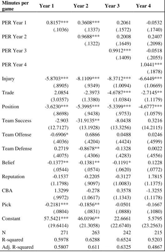
As previously discussed, due to rookie scale contracts, pick is only a perfect proxy for salary during the first four years among first round picks. Therefore, the sample was limited only to first rounders. As seen in Table 6, pick was insignificant after Year 2. Contemporaneous PER was generally significant but the effects of lagged PER were mostly indeterminate. In Year 2 and Year 4 the adjusted R-squared values were higher than with all players while it was slightly lower in Year 3. Altogether, the additional controls and cumulative performance measures led to decreased evidence of escalation. In fact there was little evidence to suggest escalation past Year 2. However, limiting the sample to first round picks did not drastically change the results.

(25)

22 Table 6: Multivariate model only with first round picks

Minutes per

game Year 1 Year 2 Year 3 Year 4

PER Year 1 0.8157*** 0.3608*** 0.2061 -0.0532

(.1036) (.1337) (.1572) (.1740)

PER Year 2 0.9688*** 0.2008 0.2407

(.1322) (.1649) (.2098)

PER Year 3 0.9912*** -0.0518

(.1409) (.2055)

PER Year 4 1.0441***

(.1878)

Injury -5.8703*** -8.1109*** -8.3712*** -6.6449***

(.8905) (.9349) (1.0094) (1.0669)

Trade 2.0854 -2.3973 -4.6787*** -2.7145**

(3.0357) (1.3380) (1.0384) (1.1179)

Position -3.6230*** -5.3995*** -5.3399*** -4.6777***

(.8698) (.9438) (.9753) (1.0579)

Team Success -2.903 -31.9135** -8.0438 0.3216

(12.7127) (13.1928) (13.3256) (14.2115)

Team Offense -0.6906* 0.6866 0.0488 0.0246

(.4036) (.4204) (.4424) (.4599)

Team Defense 0.2719 -0.8678** -0.1328 0.0022

(.4075) (.4306) (.4283) (.4556)

Belief -0.1377** -0.1381** -0.1191* 0.1228

(.0544) (.0574) (.0620) (.0772)

Reputation -0.1537 -0.2205 -0.3127 1.7815

(1.1798) (.9097) (1.0083) (1.1375)

CBA 1.3299 -0.278 0.3578 -1.3255

(.9972) (1.0617) (1.1343) (1.1178)

Pick -0.2181*** -0.1856** -0.0501 -0.1667

(.0804) (.0831) (.0888) (.1080)

Constant 57.5421*** 46.0196** 22.6661 5.5795

(19.6414) (21.3058) (22.6740) (23.2563)

N 271 263 242 215

R-squared 0.5978 0.6288 0.6524 0.5203

Adj. R-squared 0.5807 0.611 0.6325 0.4867

(26)

23 Table 7: Logistic model separated by CBA

Retained by

draft team Year 2 Year 3 Year 4

1999 CBA 2005 CBA 1999 CBA 2005 CBA 1999 CBA 2005 CBA

PER Year 1 0.1429*** 0.0495 0.0561 0.0658 0.0715 -0.0217

(.0433) (.0427) (.0510) (.0465) (.0543) (.0691)

PER Year 2 0.2082*** 0.0428 0.0506 0.1228

(.0516) (.0370) (.0582) (.0750)

PER Year 3 0.2001*** 0.0778

(.0574) (.0728)

Position 0.8626** 0.5984 0.4145 0.5498 0.0747 -0.2048

(.3912) (.4586) (.3579) (.3847) (.3688) (.4582)

Team

Success -3.0100 -3.7212 -1.5216 4.3249 5.0906 -0.9894

(5.5982) (5.2579) (4.7362) (5.6058) (5.0555) (6.2091)

Team

Offense 0.1194 0.0653 0.1206 -0.0680 -0.1402 0.1064

(.1785) (.1648) (.1543) (.1746) (.1625) (.2037)

Team

Defense -0.2135 -0.1739 -0.1076 0.0283 0.0861 -0.2239

(.1851) (.1692) (.1526) (.1891) (.1541) (.1998)

Round 1.1696* 0.6390 1.7648** -0.2138 0.9766* -1.4463

(.6482) (.7347) (.6968) (.7076) (.7165) (.8610)

Belief 0.0163 -0.0184 0.0606*** -0.0084 0.0252 -0.0119

(.0148) (.0176) (.0187) (.0196) (.0181) (.0240)

Reputation 0.2915 0.9707** -0.1953 0.9466** 0.1778* 0.9501*

(.3453) (.4542) (.3506) (.4013) (.3664) (.5374)

Pick -0.0344 -0.0128 -0.0533* -0.0345 -0.0211 -0.05

(.0238) (.0278) (.0275) (.0298) (.0287) (.0358)

Constant 10.2734 14.0127 -5.1622 1.3391 -2.4036 12.1265

(7.7964) (10.7675) (6.9002) (11.2719) (7.5709) (12.7470)

N 248 182 219 159 193 136

Pseudo

R-squared 0.2196 0.1926 0.2482 0.1444 0.2273 0.1842

(27)

24

(prob>chi2=.0835) but was highly significant thereafter. However, the pseudo R-squared values were lower than when both rounds were included. Pick was significant at the 10% level in Year 3, but there was no significant effect of CBA. Altogether, pick’s reduced significance and lack of significance past Year 2 in the multivariate regression (Table 6) suggest little escalation among first round players.

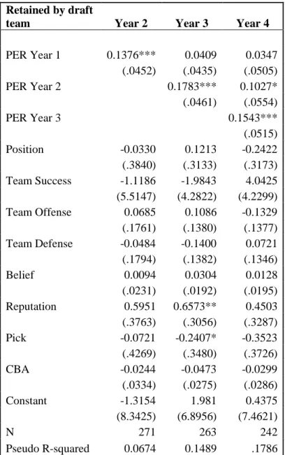
Table 8: Logistic model with only first round picks Retained by draft

team Year 2 Year 3 Year 4

PER Year 1 0.1376*** 0.0409 0.0347

(.0452) (.0435) (.0505)

PER Year 2 0.1783*** 0.1027*

(.0461) (.0554)

PER Year 3 0.1543***

(.0515)

Position -0.0330 0.1213 -0.2422

(.3840) (.3133) (.3173)

Team Success -1.1186 -1.9843 4.0425

(5.5147) (4.2822) (4.2299)

Team Offense 0.0685 0.1086 -0.1329

(.1761) (.1380) (.1377)

Team Defense -0.0484 -0.1400 0.0721

(.1794) (.1382) (.1346)

Belief 0.0094 0.0304 0.0128

(.0231) (.0192) (.0195)

Reputation 0.5951 0.6573** 0.4503

(.3763) (.3056) (.3287)

Pick -0.0721 -0.2407* -0.3523

(.4269) (.3480) (.3726)

CBA -0.0244 -0.0473 -0.0299

(.0334) (.0275) (.0286)

Constant -1.3154 1.981 0.4375

(8.3425) (6.8956) (7.4621)

N 271 263 242

Pseudo R-squared 0.0674 0.1489 .1786

(28)

25

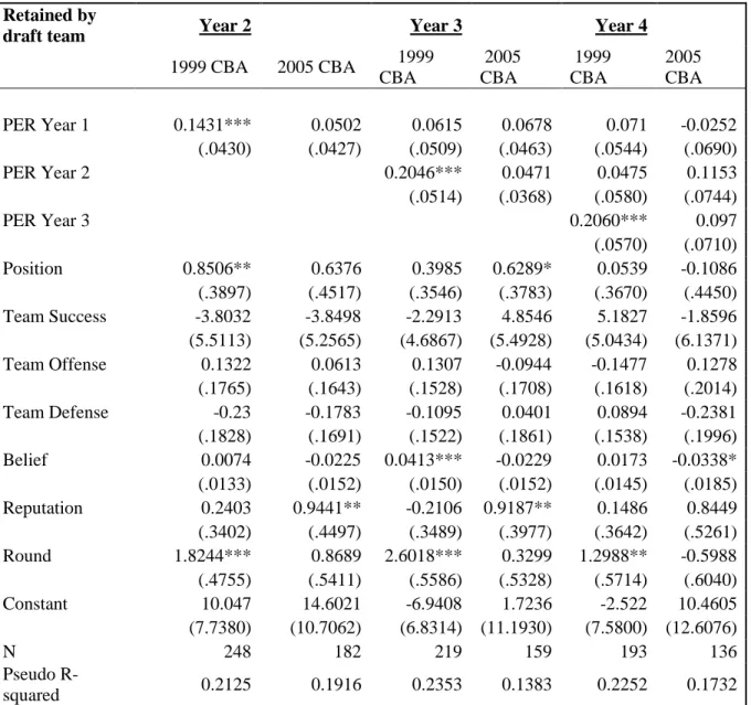
As mentioned earlier, rookie scale contracts are not only a relatively small part of a team’s payroll, but they are also exempt from the salary cap. Therefore, it is possible that the

differences in first round salaries are relatively minor, and thus commitment among all first round players is effectively equal. If this is assumed true, escalation could still exist if round affects retainment. As seen in Table 9, when pick was removed, round was significant in all years under the 1999 CBA but was never significant under the 2005 CBA. These results suggest that being drafted in the first round affected chances of survival under the 1999 CBA but did not affect odds of retainment under the 2005 CBA. As previously mentioned, the 1999 CBA

guaranteed three year contracts to first rounders while the 2005 CBA guaranteed two years. The results indicate that first round picks under the 1999 CBA were more likely than second round players to be retained through their guaranteed years. Furthermore, first round picks also were more likely to be retained for their optional fourth year. However, since there was no

(29)

26 Table 9: Logistic model without Pick variable separated by CBA

Retained by

draft team Year 2 Year 3 Year 4

1999 CBA 2005 CBA

1999 CBA 2005 CBA 1999 CBA 2005 CBA

PER Year 1 0.1431*** 0.0502 0.0615 0.0678 0.071 -0.0252

(.0430) (.0427) (.0509) (.0463) (.0544) (.0690)

PER Year 2 0.2046*** 0.0471 0.0475 0.1153

(.0514) (.0368) (.0580) (.0744)

PER Year 3 0.2060*** 0.097

(.0570) (.0710)

Position 0.8506** 0.6376 0.3985 0.6289* 0.0539 -0.1086

(.3897) (.4517) (.3546) (.3783) (.3670) (.4450)

Team Success -3.8032 -3.8498 -2.2913 4.8546 5.1827 -1.8596

(5.5113) (5.2565) (4.6867) (5.4928) (5.0434) (6.1371)

Team Offense 0.1322 0.0613 0.1307 -0.0944 -0.1477 0.1278

(.1765) (.1643) (.1528) (.1708) (.1618) (.2014)

Team Defense -0.23 -0.1783 -0.1095 0.0401 0.0894 -0.2381

(.1828) (.1691) (.1522) (.1861) (.1538) (.1996)

Belief 0.0074 -0.0225 0.0413*** -0.0229 0.0173 -0.0338*

(.0133) (.0152) (.0150) (.0152) (.0145) (.0185)

Reputation 0.2403 0.9441** -0.2106 0.9187** 0.1486 0.8449

(.3402) (.4497) (.3489) (.3977) (.3642) (.5261)

Round 1.8244*** 0.8689 2.6018*** 0.3299 1.2988** -0.5988

(.4755) (.5411) (.5586) (.5328) (.5714) (.6040)

Constant 10.047 14.6021 -6.9408 1.7236 -2.522 10.4605

(7.7380) (10.7062) (6.8314) (11.1930) (7.5800) (12.6076)

N 248 182 219 159 193 136

Pseudo

R-squared 0.2125 0.1916 0.2353 0.1383 0.2252 0.1732

(30)

27

VI. Conclusion

By incorporating recent theoretical literature and considering the current NBA labor environment, this study predicted that there would be evidence of little, if any, escalation of commitment. Furthermore, it sought to improve the data sample by limiting it to observations where draft position was predictably related to salary, i.e. “commitment.” Rejecting the suitability of an event history analysis, this study employed a logistic model designed to offer insight not provided by the previous studies. The study predicted that while draft pick may lead to increased playing time, escalation would not exist if draft positiondid not affect teams’ decisions to retain their young players. If this hypothesis proved correct, escalation of commitment would be rejected.

In this study cumulative performance measures and additional controls not only provided more predictive power of playing time and retainment but also reduced pick’s effects. However, a coach or GM change did not lead to less escalation and thus there was no evidence of

reputational concerns. In fact, on many occurrences there was evidence that an executive change positively affected a player’s odds of survival and playing time. In accordance with expectations,

when the sample was limited to the first round, pick lost much of its predictive value which suggests that team behavior is similar among first round players. In the multivariate model there was a significant effect only in Year 2 and only at the 5% level. Furthermore, the logistic model provided no direct relationship between pick and probability of retainment. However, under the 1999 CBA guaranteed money increased not only the likelihood of retainment during the

(31)

28

Reference List

Arkes, H. R., & Blumer, C. (1985). The psychology of sunk cost. Organizational Behavior and Human Decision Processes,35(1), 124–140.

Berri, D. J. (2000). Who is the “Most Valuable”? Measuring the Player’s Production of Wins in the National Basketball Association. Managerial and Decision Economics, 20(8), 411– 427.

Berri, D. J., & Bradbury, J. C. (2010). Working in the Land of the Metricians. Journal of Sports Economics, 11(1), 29–47.

Berri, D. J., Brook, S. L., & Fenn, A. J. (2011). From college to the pros: predicting the NBA amateur player draft. Journal of Productivity Analysis, 35(1), 25–35.

Berri, D. J., Schmidt, M. B., & Brook, S. L. (2004). Stars at the Gate: The Impact of Star Power on NBA Gate Revenues. Journal of Sports Economics, 5(1), 33–50.

Berri, D. J., & Simmons, R. (2011). Catching a draft: on the process of selecting quarterbacks in the National Football League amateur draft. Journal of Productivity Analysis, 35(1), 37– 49.

Boehne, D., & Paese, P. (2000). Deciding Whether to Complete or Terminate an Unfinished Project: A Strong Test of the Project Completion Hypothesis. Organizational Behavior and Human Decision Processes, 81(2), 178–194.

Boulier, B. L., Stekler, H. O., Coburn, J., & Rankins, T. (2010). Evaluating National Football League draft choices: The passing game. International Journal of Forecasting, 26(3), 589–605.

Camerer, C. F., & Weber, R. A. (1999). The econometrics and behavioral economics of

escalation of commitment: a re-examination of Staw and Hoang’s NBA data. Journal of Economic Behavior & Organization, 39, 59–82.

Chen, A. (2013, May 11). How the Mind and Body React to Watching Big Games; Tracking Heart Attack Rates After the Super Bowl. The Wall Street Journal.

Coon, L. (2013). NBA Salary Cap FAQ. Retrieved from http://www.cbafaq.com/salarycap.htm

Fort, R., & Quirk, J. (2004). Owner Objectives and Competitive Balance. Journal of Sports Economics, 5(1), 20–32.

(32)

29

Garland, H., Sandefur, C. A., & Rogers, A. C. (1990). De-escalation of commitment in oil exploration: When sunk costs and negative feedback coincide. Journal Of Applied Psychology, 75(6), 721-727.

Hakes, J. K., & Sauer, R. D. (2006). An Economic Evaluation of the Moneyball Hypothesis. The Journal of Economic Perspectives, 20(3), 173–185.

Hill, J. R., & Groothuis, P. A. (2001). The New NBA Collective Bargaining Agreement, the Median Voter Model, and a Robin Hood Rent Redistribution. Journal of Sports Economics, 2(2), 131–144.

Hill, J. R., & Jolly, N. A. (2012). Salary Distribution and Collective Bargaining Agreements: A Case Study of the NBA. Industrial Relations, 51(2), 342–363.

Kahane, L. H. (2012). The Oxford handbook of sports economics. Oxford ;New York: Oxford University Press.

Kahneman, D., & Tversky, A. (1979). Prospect theory: an analysis of decision under risk. Econometrics: Journal of the Econometric Society, 47(2), 263–192.

Keohane, L. H., & Shmanske, S. (2012). The economics of sports. New York: Oxford University Press.

Késenne, S. (2007). The economic theory of professional team sports : an analytical treatment. Cheltenham, UK ;Northampton, MA: Edward Elgar

Késenne, S. (2000). The Impact of Salary Caps in Professional Team Sports. Scottish Journal of Political Economy, 47(4), 422–430.

Koz, D., Fraser-Thomas, J. and Baker, J. (2012). Accuracy of professional sports drafts in predicting career potential. Scandinavian Journal of Medicine & Science in Sports, 22, 64–69.

Lowe, Z. (2013). 32 Bold Predictions for the NBA Season. Retrieved from

http://www.grantland.com/story/_/id/9860683/32-bold-predictions-2013-14-nba-season

Manier, J. (2006, October 29). The Sunk Cost Fallacy and Iraq. The Chicago Tribune.

McAfee, R. P., Mialon, H. M., & Mialon, S. H. (2010). Do Sunk Costs Matter? Economic Inquiry, 48(2), 323–336.

(33)

30

Staw, B. M. (1976). Knee-deep in the big muddy: a study of escalating commitment to a chosen course of action. Organizational Behavior and Human Performance, 16(1), 27–44.

Staw, B. M., & Hoang, H. (1995). Sunk Costs in the NBA: Why Draft Order Affects Playing Time and Survival in Professional Basketball. Administrative Science Quarterly, 40(3), 474–494.

Szymanski, S., & Kesenne, S. (2004). Competitive balance and gate revenue sharing in team sports. The Journal of Industrial Relations, 52(1), 165–177.

Tan, H.-T., & Yates, J. F. (2002). Financial Budgets and Escalation Effects. Organizational Behavior and Human Decision Processes, 87(2), 300–322.

Thaler, R. (1980). Toward a positive theory of consumer choice. Journal of Economic Behavior & Organization, 1(1)

Vrooman, J. (1995). A General Theory of Professional Sports Leagues. Southern Economic Journal, 61(4), 971–990.

Weber, M., & Camerer, C. F. (1998). The disposition effect in securities trading: an experimental analysis. Journal of Economic Behavior & Organization, 33(2), 167–184.

(34)

31

Appendix A

1. The Player Efficiency Rating is calculated as follows:

(

) [ () (

) ( ( ( (

)) () (

))) ( )

((

) (

) )]

( )

( ₎

MP=minutes played

FGA=field goal attempts

FG=field goals made

3P=three point FG made

AST=assists

FT=free throws made

TOV=turnovers

DRB%=defensive rebounding percentage

STL=steals

BLK=blocks

ORB=offensive rebound

The unadjusted PER (uPER) is then standardized to the league pace and the league average:

(35)

35 2. The Win Shares metric is calculated as follows:

Marginal offense is computed:

Then, the marginal points per win (MPW) is calculated:

( )

Then Win Shares is computed as follows,

(36)

36

Appendix B

1.

Table 1a: Variable definitions

Variable Description

Minutes per Game Minutes played per game

Retained by Draft Team If a player is retained by his drafted team for the entirety of the year then the variable is equal to 1, and equal to 0 if not.

Scoring

Toughness

Quickness

PER

Win Shares

Pick

Standardized performance index consisting of points per minute, field-goal percentage and free-throw percentage

Standardized performance index consisting of rebounds per minute and blocks per minute

Standardized performance index consisting of assists per minute and steals per minute

Player Efficiency Rating

Win Shares per 48 minutes

Player’s draft position expressed as the draft number.

Round Dummy variable equal to 1 if drafted in the first round and equal to 0 if drafted in the second round.

Belief Average of the third-party draft projections of www.nbadraft.net and ESPN draft analyst Chad Ford, both reputable experts in player evaluation.

Injury Dummy variable equal to 1 if a player missed more than 10 games during the season and equal to 0 if not.

Trade Dummy variable equal to 1 if traded or cut before or during the season and equal to 0 if not.

Position Dummy variable equal to 1 if a player is a Power Forward or Center and equal to 0 if not.

Team Success Team winning percentage, inputted as a decimal.

Team Offense Points produced per 100 possessions

(37)

37

2.

Table 2a: Descriptive statistics

Variable Observations Mean Std. Dev. Min Max

Pick 587 29.8620 16.9780 1.0000 60.0000

Belief 587 32.2010 19.5459 1.0000 61.0000

Round 587 0.4974 0.5004 0.0000 1.0000

Position 587 0.2675 0.4430 0.0000 1.0000

Year 1

Minutes per game 430 11.0642 9.8209 0.0366 38.0732

Scoring 430 0.0000 1.0000 -3.4842 3.4894

Toughness 430 0.0000 1.0000 -2.1940 2.9082

Quickness 430 0.0000 1.0000 -1.6132 3.5699

PER 430 10.9823 4.9157 -20.4000 26.0000

Win Shares 430 0.0384 0.0827 -0.3710 0.3450

Trade 430 0.0256 0.1579 0.0000 1.0000

Injury 430 0.3066 0.4615 0.0000 1.0000

Team Success 430 0.4613 0.1508 0.1585 0.8171

Team Offense 430 104.6550 3.7886 92.2000 113.9000

Team Defense 430 105.8470 3.4781 95.4000 114.7000

Reputation 430 0.1329 0.3397 0.0000 1.0000

Year 2

Minutes per game 408 14.9629 11.0349 0.0122 41.3171

Retained by Draft team 408 0.7428 0.4375 0.0000 1.0000

Scoring 408 0.0000 1.0000 -4.6811 6.3793

Toughness 408 0.0000 1.0000 -2.2448 2.7208

Quickness 408 0.0000 1.0000 -1.6694 5.1444

PER 408 12.2909 6.5227 -48.6000 53.0000

Win Shares 408 0.0645 0.1214 -1.2640 0.7100

Trade 408 0.2641 0.4412 0.0000 1.0000

Injury 408 0.2470 0.4316 0.0000 1.0000

Team Success 408 0.4705 0.1413 0.1463 0.8049

Team Offense 408 105.1951 3.6933 92.2000 115.3000

Team Defense 408 106.1066 3.5041 95.4000 114.7000

Reputation 408 0.3407 0.4744 0.0000 1.0000

Year 3

Minutes per game 378 17.0086 11.6729 0.1098 40.9878

Scoring 378 0.0000 1.0000 -4.7772 3.4567

Toughness 378 0.0000 1.0000 -2.1236 3.9197

Quickness 378 0.0000 1.0000 -1.6943 4.6050

PER 378 13.2471 5.4148 -9.0000 35.3000

(38)

38 Table 2a (continued): Descriptive statistics

Trade 378 0.4770 0.4999 0.0000 1.0000

Injury 378 0.2351 0.4244 0.0000 1.0000

Team Success 378 0.4818 0.1439 0.1463 0.8171

Team Offense 378 105.7622 3.5727 92.2000 115.3000

Team Defense 378 106.2654 3.5609 94.1000 114.4000

Reputation 378 0.4634 0.4991 0.0000 1.0000

Year 4

Minutes per game 327 18.8302 10.5495 0.0366 41.1342

Scoring 327 0.0000 1.0000 -5.2204 2.3003

Toughness 327 0.0000 1.0000 -2.1655 3.8521

Quickness 327 0.0000 1.0000 -1.6162 4.1431

PER 327 14.1844 5.9642 -54.4000 33.3000

Win Shares 327 0.0886 0.0991 -1.3120 0.2950

Trade 327 0.5963 0.4911 0.0000 1.0000

Injury 327 0.1925 0.3946 0.0000 1.0000

Team Success 327 0.4894 0.1418 0.1061 0.8171

Team Offense 327 105.9805 3.4517 95.2000 114.5000

Team Defense 327 106.3539 3.3660 94.1000 114.7000

Reputation 327 0.4600 0.4988 0.0000 1.0000

Year 5

Minutes per game 299 20.0106 11.0884 0.0488 41.2683

Scoring 299 0.0000 1.0000 -4.8258 4.1788

Toughness 299 0.0000 1.0000 -2.0699 3.1860

Quickness 299 0.0000 1.0000 -1.7246 4.1299

PER 299 14.9268 4.5551 3.7000 35.2000

Win Shares 299 0.1031 0.0622 -0.0860 0.4840

Trade 299 0.6678 0.4714 0.0000 1.0000

Injury 299 0.1465 0.3539 0.0000 1.0000

Team Success 299 0.5058 0.1463 0.1585 0.8049

Team Offense 299 106.4754 3.3931 99.0000 115.3000

Team Defense 299 106.2148 3.5835 94.1000 114.7000

Reputation 299 0.5860 0.4930 0.0000 1.0000

Year 6

Minutes per game 249 20.5452 10.0556 0.0610 39.3537

Scoring 249 0.0000 1.0000 -3.4585 2.5814

Toughness 249 0.0000 1.0000 -2.2255 3.0159

(39)

39 Table 2a (continued): Descriptive statistics

PER 249 14.5438 4.9018 -4.8000 33.0000

Win Shares 249 0.0956 0.0643 -0.1790 0.3180

Trade 249 0.7019 0.4578 0.0000 1.0000

Injury 249 0.1431 0.3505 0.0000 1.0000

Team Success 249 0.4876 0.1497 0.1061 0.8171

Team Offense 249 106.4357 3.2563 95.2000 114.5000

Team Defense 249 106.9176 3.2529 98.2000 114.4000