Time Series Predictive Analysis of Bitcoin with ARMA-GARCH
model in Python and R
Honor Thesis submitted by
Jiayi Ding
Advisor: Professor Chuanshu Ji
University of North Carolina at Chapel Hill
Abstract:
Bitcoin arises recent years as a most successful and widely used cryptocurrency. Though it was
first invented as a decentralized currency, Bitcoin has become more and more popular as a
financial asset with a market capitalization of around $117 billion, as increasing number of
investors and portfolio managers start to invest in and trade it. In this paper, we are interested in
finding out the future course of Bitcoin prices and returns and examining the predictive power of
the ARMA- GARCH model. The paper uses Python and R environment to analyze and model
financial time series. The first part covers the preliminary analysis of the daily closing prices and
returns of Bitcoin, and also the stationarity of the return series. The second part intends to fit an
appropriate ARMA-GARCH model. The last part focuses on using fitted model to predict future
returns and prices of Bitcoin and compare it to our validation dataset.
1. Background
Bitcoin is a cryptocurrency first introduced by Nakamoto in his paper “Bitcoin: A Peer-to-Peer
Electronic Cash System” in 2008[1]. A cryptocurrency can be defined as “a virtual coinage
system that functions much like a standard currency, enabling users to provide virtual payment
for goods and services free of a central trusted authority” [2]. Three unique features of
cryptocurrencies are that they are fully decentralized and depend on cryptographic protocols, or
extremely complex code systems that encrypt sensitive data transfers to secure their units of
exchange, and also control the finite supply. Bitcoin is the first widely used and traded
cryptocurrency since 2009, when the Bitcoin software started to be available to the public and
mining- the process of which new bitcoins can be created and transactions can be recorded and
decentralized and encrypted currencies catch on, more rival, alternative cryptocurrencies appear.
But Bitcoin remains the most successful and widely accepted cryptocurrency with a market cap
at $117 billion, representing about 45% of the total estimated cryptocurrency capitalization at
present (coinmarketcap.com accessed on Mar 30th 2018).
A few studies have already been conducted on the financial and statistical characteristics of
Bitcoin. One group of economists has been focusing on price discovery in the Bitcoin market, for
example, Brandvold et al. [3] and Bouoiyour et al. [4] reveal some lead-lag relationship between
Bitcoin prices, transactions use, and investors’ attractiveness. Other studies also show that
Bitcoin price is subject to unique factors which are substantially different from those affecting
conventional, financial assets, such as internet search [5], information on google trends, and
word-of-mouth information on social media.[6] In fact, as Bitcoin is mainly used and viewed as
an asset rather than a currency [7], and the Bitcoin market is currently highly speculative, and
more volatile and susceptible to speculative bubbles than other currencies [8][9]. Moreover, the
presence of long memory and persistent volatility [10] justifies the application of GARCH-type
models.
The purpose of this paper is to utilize time series techniques to predict the future returns and
prices of Bitcoin. At the same time, we want to examine the effectiveness of the popular ARMA-
GARCH model in economics and financial world. As Bitcoin gradually has had a place in the
financial markets and in portfolio management [11], time series analysis is a useful tool to study
the characteristics of Bitcoin prices and returns, and extract meaningful statistics in order to
2. Data
The data used to fit the model are the daily closing prices of Bitcoin from July 18th, 2010 ( as the
earliest data available) to Jan 30th, 2018, which corresponds to a total of 2754 observations. We
save the data from Jan 31st, 2018 to March 31st, 2018 to perform validation latter. The data is
compiled from Bitstamp, the largest Bitcoin exchange, and covers a daily database denominated
in US dollar, which is the main currency against which Bitcoin is the most traded. We calculate
the log-returns by taking the natural logarithm of the ratio of two consecutive prices, as a good
approximation of daily percentage changes in prices.
3. Preliminary analysis and results
3.1 Descriptive Statistics
Since its introduction in 2009, the value of Bitcoin grew rapidly and its price achieved all time
high: $19, 340 at the end of 2017. However, it recently has been traded lower to $6,000 to
$7,000 range in the past month. Table 1 reports the descriptive statistics of the returns of Bitcoin,
with the maximum daily return in the sample being 0.4246, the minimum being -0.4915, an
standard deviation of 0.0588. The result of the Jarque-Bera statistic indicates the departure from
normality. The returns are also negatively skewed, while the excess kurtosis suggests evidence of
a leptokurtic distribution.
3.2 Check Stationarity
Before modeling time index data, we need to check the stationarity, as a lot of statistical and
econometric methods are based on stationarity. Based on the results of the Augmented Dickey–
Fuller (ADF) tests as shown in Table 2, we fail to accept the null hypothesis of a unit root for the
returns, and, hence, stationarity is guaranteed for the log-return series of Bitcoin.
4. Methodology
One common observation we get out of the economic and financial data is volatility clustering.
Suppose we have noticed that recent daily returns have been unusually volatile. We might expect
that tomorrow’s return is also more variable than usual. We can also observe that the squared
returns of an asset are usually positively auto-correlated, i.e. if an asset price made a big move
yesterday, it is more likely to make a big move today. With economic and financial data,
varying volatility is more common than constant volatility, and accurate modeling of
time-varying volatility is of great importance.
4.2 Justifications for ARMA-GARCH model
In our case, we have already known from the excess kurtosis that an obvious fat tails displayed in
our series, a typical evidence of heteroskedastic effects as clustering of volatility. We can also
observe from the squared log-return. Fig.5 illustrates that the squared returns appear to fluctuate
around a constant level, but exhibit volatility clustering. Large changes in the squared returns
tend to cluster together, and small changes tend to cluster together, which also indicates that the
series exhibits conditional heteroscedasticity.
It is even more clear, if we plot the sample autocorrelation function (ACF) and partial
The sample ACF and PACF show significant autocorrelation in the squared log-return series.
Then, a Ljung-Box Q-test can more formally assess autocorrelation.
Table 3. Results of Ljung-Box Q-test
lag p-value Q c-value rejectH0
1 0.0000 2756.729 2.706 TRUE
2 0.0000 5513.13 4.605 TRUE
11 0.0000 26379.902 17.275 TRUE
12 0.0000 28561.907 18.549 TRUE
13 0.0000 30740.143 19.812 TRUE
14 0.0000 32914.629 21.064 TRUE
15 0.0000 35076.471 22.307 TRUE
16 0.0000 37238.845 23.542 TRUE
As illustrated in the ACF and PACF plot of squared returns and the results of Ljung-Box test,
there is clearly autocorrelation present. The model we are going to look at will attempt to capture
the autocorrelation of squared returns, clustering volatility, as well as the heteroscedasticity. The
significance of the lags in both the ACF and PACF indicate we need both AR and MA
components for our model. As we know that ARMA models are used to model the conditional
mean of the process given past information, which however, assumes the conditional variance
given the past is constant. ARMA model alone fails to capture the volatility clustering behavior.
Thus, we will use GARCH process that has become widely used in econometrics and finance, to
correct the heavy tails and model the randomly varying volatility in Bitcoin’s return.
We describe the mean equation of the log-return series 𝑟" by the process
𝑟"= 𝐸(𝑟"|𝑟"'(, 𝑟"'*, … ) + 𝜀" ,
where 𝐸(𝑟"|𝑟"'(, 𝑟"'*, … ) denotes the conditional expectation operator. 𝜀" denotes the
innovations or residuals of the log-return series with zero mean, and plays the role of the
unpredictable part of the time series, generated from a GARCH process. We first model the
mean equation as an ARMA process.
4.3 ARMA process
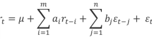
Recall that the ARMA(m, n) process of autoregressive order of m, and moving average order n
𝑟"= 𝜇 + 1 𝑎3𝑟"'3 4
35(
+ 1 𝑏7𝜀"'7 8
75(
+ 𝜀"
With mean 𝜇, autoregressive coefficients 𝑎3, and moving average coefficients 𝑏7.
To choose the best order(m, n) , we try out different combinations and select the one with the
lowest AIC and BIC in Python. Table 4 illustrates ARMA(2,1) performs best, and shows the
estimated coefficients results for ARMA(2,1).
Table 4. AIC and BIC of ARMA (m,n)
Order AIC
(0,1) -7791.96
(0,2) -7796.68
(1,0) -7792.15
(1,1) -7798.64
(1,2) -7843.69
(2,0) -7795.67
(2,1) -7836.96
(2,2) -7807.82
ARMA(1,2)
Residuals:
Min 1Q Median 3Q Max
-0.487415 -0.016283 -0.002524 0.018147 0.422052
Coefficient(s):
Estimate Std. Error t value Pr(>|t|)
ar1 -0.914004 0.019341 -47.257 < 2e-16 ***
ma1 0.962524 0.027655 34.805 < 2e-16 ***
ma2 0.040547 0.019782 2.050 0.04039 *
intercept 0.008478 0.002216 3.826 0.00013 ***
---
Next, we need to check the residuals after fitting ARMA(2,1), which should be align with our
4.4 GARCH Process
As we already detect the autocorrelation effects in our residual/innovation series, we now need to
apply GARCH (p,q) model in order to estimate the conditional variance going forward, using:
𝜀" = 𝑧"𝜎"
𝜎"* = 𝛾𝑉
=+ 1 𝛼3 ?
35(
𝜀"'3* + 1 𝛽 3 A
75(
𝜎"'7*
where
𝜎"* = 𝑉𝑎𝑟(𝜀
"|𝜀"'(, 𝜀"'*, … )
denotes the conditional variance and 𝑧" is a noise term iid ~(0,1) .
Three parameters (𝛾, 𝛼, 𝛽) must satisfy that
𝛾 + 𝛼 + 𝛽 = 1
If we introduce a new parameter 𝜔 to denote the weighted average long-term variance, where
𝜔 = 𝛾𝑉=
𝜎"* = 𝜔 + 1 𝛼 3 ?
35(
𝜀"'3* + 1 𝛽 3 A
75(
𝜎"'7*
The model tells us that tomorrow’s variance is a function of today’s squared innovations, today’s
variance, and the weighted average long-term variance.
The estimation of (𝜔, 𝛼, 𝛽) can be conducted utilizing the maximum likelihood method, which is
an iterative process by looking for the maximum value of the sum among all sums defined as:
1 [− ln(𝜎3*) −𝜀3* 𝜎3*] I
35J
where N denotes the length of the innovation or residuals series {𝜀7} (j=2,…, N)
To choose the best order(p, q) , we try out different combinations and make the decision based
on Log-Likelihood, and Information Criteria. Fig.12 gives us ARMA(1,2)-GARCH(1,2) as the
best model.
Table 5. Log Likelihood and Information Criteria of ARMA(1,2)-GARCH(p,q)
Model (p,q) Log-Likelihood AIC BIC HQIC
(1,1) 5245.095 -3.8039 -3.7846 -3.7969
(1,2) 5248.175 -3.8054 -3.7839 -3.7977
(1,3) 5248.156 -3.8047 -3.7810 -3.7961
(2,1) 5245.124 -3.8032 -3.7817 -3.7954
(2,2) 5248.159 -3.8047 -3.7810 -3.7961
(2,3) 5248.150 -3.8040 -3.7782 -3.7946
(3,1) 5244.112 -3.8018 -3.7781 -3.7932
(3,2) 5247.063 -3.8032 -3.7774 -3.7938
Fig 12. Full model parameters
Mean Model: ARMA(1,2)
Variance Model: GARCH(1,2)
Optimal Parameters
---
Estimate Std. Error t value Pr(>|t|)
mu 0.001368 0.000090 15.2490 0
ar1 0.965530 0.003229 299.0540 0
ma1 -0.983092 0.000887 -1107.7277 0
ma2 0.030457 0.000260 117.1919 0
omega 0.000057 0.000009 6.0399 0
alpha1 0.278171 0.019459 14.2952 0
beta1 0.461024 0.025163 18.3215 0
beta2 0.259804 0.020355 12.7637 0
So far, we have successfully obtained the full ARMA(1,2)-GARCH(1,2) model:
𝑟"= 0.001368 + 0.965530𝑟"'(+ (−0.983092)𝜀"'(+ 0.030457𝜀"'*+ 𝜀"
𝜀" = 𝑧"𝜎", 𝑧"~𝑖𝑖𝑑(0,1)
𝜎"* = 0.000057 + 0.278171 𝜀
"'(* + 0.461024𝜎"'(* + 0.259804𝜎"'**
5. Forecasting
5.1 Validation Dataset
After obtaining the fitted ARMA-GARCH model, we are curious about how the model would
perform in predicting the future prices of Bitcoin. Here we load the saved validation dataset, i.e.
the daily closing prices for Bitcoin from Jan 31st, 2010 to March 31st, 2018, and calculate the
daily log-returns during such period. -0.6
-0.4 -0.2 0 0.2 0.4 0.6
5.2 Forecasting results
Using the methodology we describe earlier and resulted ARMA(1,2)-GARCH(1,2) model, we
are able to forecast the future prices (from 2010-07-18 to 2018-01-30) for Bitcoin. The graphs
Compared with the actual prices, our model can roughly predict the ups and downs of Bitcoin’s
return/price movement. However, it fails to capture the high volatility of the daily return/price
and thus gives a prediction around a rather constant level relative to the actual return/price. We
can also use a numeric measurement to judge how well our model performs across time:
𝑀𝑆𝑃𝐸 = 1
𝑀 1 (𝑃4" − 𝑋")*
^
45(
where MSPE stands for “Mean Squared Prediction Error”; M stands for the number of
simulations; 𝑃4" stands for the prediction return/price at time t for simulation m; 𝑋" stands for
We can follow the same procedure to fit different models on different datasets. For example, the
following two pairs of graphs report the best models resulting from different sets of data used. If
we use the closing price of Bitcoin from 2017-1-1 to 2018-3-30, which corresponds to the period
when Bitcoin starts to draw public attention and become popular among investors, the best
possible model is ARMA(2,5)-GARCH(1,3). The following graphs show the prediction result
We can tell that ARMA(2,5)-GARCH(1,3) fails to predict the both the level and trend of future
Bitcoin price. That means for our case using a more recent dataset doesn’t improve our results of
prediction of Bitcoin price. However, it does better than ARMA(1,2)-GARCH(1,2) model in
forecasting the future volatility in returns, especially for a longer period, by comparing the
MSPE of ARMA(2,5)-GARCH(1,3) with that of ARMA(1,2)-GARCH(1,2).
6. Conclusions
GARCH modeling builds on advances in the understanding and modeling of volatility. It takes
characteristics of financial time series, which are also observable in the Bitcoin case. It’s
theoretically able to provide accurate forecasts of variances and covariances of returns through
modeling time-varying conditional variances. As a consequence, GARCH models have become
quite popular in diverse fields as risk management, portfolio management and asset allocation,
option pricing, foreign exchange, and the term structure of interest rates.[12]
In this paper, we intend to predict the future prices of Bitcoin, one of the most widely used and
traded cryptocurrency, and study the predictive power of ARMA-GARCH model on the Bitcoin
return/price series. From the predicted results, we have realized that although GARCH models
are useful across a wide range of financial and economical applications, they are not a quite
effective and suitable model candidate in studying the Bitcoin return/price series. One of the
main reasons is that GARCH models are parametric specifications that operate best under
relatively stable market conditions[13]. Although GARCH is explicitly designed to model
time-varying conditional variances, GARCH models often fail to capture highly irregular phenomena,
including wild market fluctuations (e.g., crashes and subsequent rebounds), and other highly
unanticipated events that can lead to significant structural change, which are exactly what has
been going on in the Bitcoin market recently. Events and factors such as the recent
announcement by Google, that it will put a ban on all cryptocurrency related ads, the collapsed
cryptocurrency exchangeMt. Gox, increasingly hostile regulatory climate in China, increased
regulatory scrutiny of ICOs, banks are also putting more and more pressure on the market by
barring their customers from purchasing cryptocurrencies using their plastic cards, all
contributed towards uncertainty, geopolitical risks, and wild fluctuations in the Bitcoin market.
such as asymmetric GARCH, EGARCH, TGARCH, etc. hopefully to capture the characteristics
of the Bitcoin series, and make a better prediction.
Reference:
[1] Satoshi Nakamoto (2008). Bitcoin: A Peer-to-Peer Electronic Cash System. URL:
https://bitcoin.org/bitcoin.pdf
[2]Farell, Ryan (2015). An Analysis of the Cryptocurrency Industry. Wharton Research
Scholars. 130. URL: https://repository.upenn.edu/wharton_research_scholars/130
[3] Brandvold, M., Molnár, P., Vagstad, K., and Valstad, O. C. A. (2015). Price discovery on
Bitcoin exchanges. Journal of International Financial Markets, Institutions and Money 36: 18–
35. URL: http://www.sciencedirect.com/science/article/pii/S104244311500027X
[4] Bouoiyour, J., Selmi, R., Tiwari, A.K. and Olayeni, O.R. (2016). What drives Bitcoin price?.
Economics Bulletin 36(2): 843–850. URL:
http://www.accessecon.com/Pubs/EB/2016/Volume36/EB-16-V36-I2-P82.pdf
[5] Kristoufek, L. (2013). Bitcoin meets Google Trends and Wikipedia: Quantifying the
relationship between phenomena of the Internet era. Scientific Reports, 3, 3415
[6] Garcia, D., Tessone, C., Mavrodiev, P. and Perony, N. (2014). The digital traces of bubbles:
Feedback cycles between socio-economic signals in the Bitcoin economy. Journal of the Royal
[7] Glaser, F., Zimmermann, K., Haferkorn, M., Weber, M. C. and Siering, M. (2014). Bitcoin-
Asset or Currency? Revealing Users' Hidden Intentions. Revealing Users' Hidden Intentions.
ECIS. Available at SSRN: 2425247.
[8]Grinberg, R., 2011. Bitcoin: An innovative alternative digital currency. Hastings Sci.
Tech. LJ. 4, 160–211 Available at SSRN: https://ssrn.com/abstract=1817857.
[9] Cheah, E.T., Fry, J., 2015. Speculative bubbles in Bitcoin markets? An empirical
investigation into the fundamental value of Bitcoin. Econom. Lett. 130, 32–36.
http://dx.doi.org/10.1016/j.econlet.2015.02.029.
[10] Bariviera, A.F., Basgall, M.J., Hasperu., W., Naiouf, M., 2017. Some stylized facts of
the Bitcoin market. Physica A 484, 82–90.
[11] Dyhrberg, A.H., 2016a. Bitcoin, gold and the dollar - A GARCH volatility analysis.
Financ. Res. Lett. 16, 85–92. https://doi-org.lcproxy.shu.ac.uk/10.1016/j.frl.
2015.10.008.
[12] Bollerslev, T., R.Y. Chou, K.F. Kroner, "ARCH Modeling in Finance: A Review of the
Theory and Empirical Evidence," Journal of Econometrics, Vol. 52, pp. 5-59, 1992.