Managing Customer Arrivals in Service Systems
with Multiple Servers
Christos Zacharias
Department of Management Science, School of Business Administration, University of Miami, Coral Gables, FL 33146.
Michael Pinedo
Department of Information, Operations & Management Sciences, Stern School of Business, New York University, New York, NY 10012.
We analyze a discrete multi-server model for scheduling customer arrivals under no-shows. Customers may have different waiting cost coefficients and different no-show rates, reflecting their type and their history in attending scheduled appointments respectively. The challenge is to assign customers to time slots so that the service system utilizes its resources efficiently, and customers experience short waiting times. Theoretical and heuristic guidelines are provided for the effective practice of appointment overbooking to offset no-shows. For the case of heterogeneous customers, we provide structural properties of an optimal schedule and we introduce a new sequencing rule. When customers come from a homogeneous pool, recursive expressions for the performance measures of interest are derived and we provide an upper bound for the optimal overbooking level. Extensive numerical experiments reveal further properties and patterns that appear in the optimal solution, and motivate the development of two very well performing and computationally inexpensive heuris-tic solutions. Our analysis demonstrates the benefits of resource-pooling in containing operational costs and increasing customer throughput.
Key words: service systems; scheduling; no-shows; overbooking; discrete queues; parallel servers.
History: working paper, last edited on August 15 2015.
1. Introduction
Appointment scheduling systems are widely used as a tool for managing customer arrivals and matching supply and demand for services. It is common for customers to not show up for their scheduled services. Missed appointments result in under-utilization of a service system’s valuable resources and limit the access for other customers who could have filled the empty slots.
Appointment overbooking is one operational strategy employed by service providers to address the issue of no-shows and at the same time increase customers’ access to services. On the other hand, overbooking potentially results in an overcrowded facility, with increased customers’ waits and system’s overtime. In this study we demonstrate that a sensible practice of appointment over-booking can significantly improve the operational performance of a service system, while customers experience short waiting times and better access services.
We address the problem of scheduling customer arrivals at a parallel-server system under no-shows. Customers have different waiting cost coefficients and different no-show rates, reflecting
their type and their history in attending scheduled appointments respectively. An optimal sched-ule balances the trade-offs between the benefits of efficient resource utilization and the costs of customers’ waiting time.
This study demonstrates that an informed strategy for appointment overbooking can significantly improve the operational performance of a service system, while customers experience short waiting times and better access to care. A discrete queueing model captures the random evolution of the system’s workload, based on which we derive recursive expressions for the performance measures of interest. The task of finding an optimal schedule is modeled as an integer stochastic program which is analytically intractable and computationally expensive. A tight upper-bound (a solution to a convex program) restricts our search for an optimal schedule on a contained solution space. Our theoretical and experimental analysis reveals properties and patterns that appear in the optimal scheduling strategy, and informs the development of two highly efficient heuristic solutions.
While motivated by the pressing needs of the healthcare sector, our model is applicable for a wide range of service systems with appointment driven arrivals. We avoid a reference to a particular application domain throughout this study, by using generic terms as “servers” and “service system”. In outpatient care, our “service system” can be used to model a diagnostic facility where it is crucial to utilize resources (e.g., CT scan, X-ray generator, MRI) efficiently. Doctors are modeled as “parallel servers” in settings where continuity of care (see Balasubramanian et al. (2010)) is not a concern. Nurses are modeled as “parallel servers” when they are the bottleneck resource, and/or the presence of a doctor is not required (e.g., vaccination and immunization, routine lab testing, etc.). Other application domains include in-office consultation (e.g., financial, legal), on-site customer support (e.g., Apple Genius Bar), entertainment, cosmetic services.
2. Related Literature
Many papers have appeared in the literature on appointment scheduling, mostly motivated by healthcare applications. Cayirli and Veral (2003), Gupta and Denton (2008) provide overviews of the literature, the research challenges and opportunities. Hall (2012) provides a comprehensive review of models and methods used for scheduling the delivery of patient care for all parts of the healthcare system. The analysis may be based on anyone of a variety of approaches, including stochastic programming (e.g., Mancilla and Storer (2012), Mak et al. (2014)), queueing theory (e.g., Green and Savin (2008), Liu and Ziya (2013), Kuiper et al. (2014)), and stylized scheduling models (e.g., Robinson and Chen (2010), LaGanga and Lawrence (2012), Zacharias and Pinedo (2014)).
In the case of homogeneous customers it is of interest to determine how many customers to schedule any given day and how to allocate these customers to slots. The sequencing of the cus-tomers is also of interest when cuscus-tomers have different characteristics. In most cases, finding an
optimal schedule is analytically intractable, and thus, the majority the literature uses enumeration, search algorithms, simulation-based techniques and/or heuristics.
A service system typically starts empty at the beginning of a working day, operates for a finite amount of time, and shuts down until the next period. Therefore, it is important to perform tran-sient analysis for the random evolution of such systems. As pointed out in Bandi and Bertsimas (2012), transient queues are difficult to analyze via classical queueing techniques. Typically the analysis of rich queueing systems over finite time horizons is addressed either by computer simu-lation (e.g., Millhiser and Veral (2014), Klassen and Yoogalingam (2009)) or approximations (e.g., Araman and Glynn (2012), Honnappa et al. (2014), Zacharias and Armony (2015)).
Most of the literature focuses on single-server models. Kaandorp and Koole (2007), Hassin and Mendel (2008), Klassen and Yoogalingam (2009), Robinson and Chen (2010), Millhiser and Veral (2014) are some recent works that consider the appointment scheduling problem with homogeneous customers who arrive on time for their scheduled appointments, if they do show up. Begen and Queyranne (2011), Cayirli et al. (2012), LaGanga and Lawrence (2012), Zacharias and Pinedo (2014) account for customer heterogeneity as well.
Even though the literature for the single server system is quite extensive, the multi-server case has received limited attention. As pointed out by Gupta and Wang (2012) as well, appointment scheduling models become intractable if multiple features are considered simultaneously. Very few studies analyze service systems with more than one server, and, to the best of our knowledge, in that case only simulation studies have been conducted. For example, Sickinger and Kolisch (2009) propose and evaluate heuristic scheduling policies for a medical center with two computer tomog-raphy (CT) scanners, Liu and Liu (1998) study a block appointment system for clinic operations with multiple random arriving doctor, Zhu et al. (2009) construct a discrete event simulation model to study specialist outpatient clinics. A stylized discrete queueing model withs≥1 servers has not been studied analytically in the literature and bears unique challenges.
The goal of this study is to develop and analyze a discrete multi-server queueing model for designing appointment systems. We address the following questions: (a) how to effectively over-book capacity in order to offset customer no-shows, (b) how to allocate the available service slots throughout the working day and furthermore, (c) how to account for patient heterogeneity. The objective function is the weighted sum of expected system’s idle time, system’s overtime and cus-tomers’ waiting time.
3. Homogeneous Customers
In this section we introduce a stylized discrete queueing model that captures the random evolution of the system’s workload over time, based on which we derive recursive expressions for the
perfor-mance measures of interest in transient state. Consequently we present the optimization problem under study and characterize the optimal overbooking strategy.
3.1. Discrete Multi-Server Scheduling Model
Consider s identical service providers working in parallel. Each one has in her regular schedulen time slots available to serve customers in a working day. Beyond thesenregular slots, each one can serve customers in overtime slots as well. The system’s regular capacity is thereforen×scustomers per day.
Customer arrivals are driven by scheduled appointments and the scheduler’s task is to assign a number of customers to each time slot. We assume that customers show up with probability p= 1−q∈(0,1) at the beginning of their assigned slot and require deterministic service of one time slot. The number of customers to be scheduled throughout the working day (a decision variable) is denoted bym, and we let y=m−n×sdenote the overbooking level.
We consider only schedules that assign all m customers to the nregular time slots. That is, no customer is assigned a priori at the outset to an overtime slot. However, if the service providers have not served all customers by the end of then-th slot, then some or all of them have to continue working overtime until the queue empties out, while overtime costs are being incurred.
Since customers are homogeneous in this section, their sequencing is irrelevant, and a schedule can be completely characterized by the vectorx= (x1, . . . , xn)∈Zn, wherextis the number of customers
assigned to slot t, with m=Pn
t=1xt. In §5 we address the optimal sequencing of heterogeneous customers.
Before we introduce the optimization problem, we characterize the random evolution of the systems workload under any given schedulex. The number of new arrivals at the beginning of each slot is a binomial random variable, not necessarily identically distributed, since we allow to assign a different number of customers to different slots. The backlog of customers at the beginning of slott, denoted byZt, is captured by the recursion
Zt= max{Zt−1+At−1−s,0}, fort≥2, (1) and Z1= 0,
whereAt∼Binomial (xt, p) denotes the number of new arrivals at slott. Our service system evolves
randomly over time as a discrete multi-server queue with group arrivals, i.e., a DAt/D/s queue.
Note that a similar recursion with (1) describes the waiting timein a D/G/1 queue, see Janssen and van Leeuwaarden (2005).
The probability distribution of the queue length in transient state is derived as follows. Let f(k;n, p) be the probability that a Binomial (n, p) random variable takes a value equal to k, i.e.,
f(k;n, p) =
n k
pk(1−p)n−k, and let πj
t(x) = Pr(Zt=j) denote the probability of a backlog of
j customers at the the beginning of slot t under schedule x. Let lt=
Pt
τ=1(xτ−s) denote the
maximum possible backlog at the beginning of slot t. Assuming that the system is empty at the beginning of the working day, then π0
1(x) = 1 and π
j
t(x) can be expressed recursively for t=
2,3, ..., n+ 1 as
πi t(x) =
min(s,lt−1) X
j=0
πt−j 1(x)
s−j
X
k=0
f(k;xt−1, p) fori= 0
min(s+i,lt−1) X
j=max(0,s+i−xt)
πt−j 1(x)f(s+i−j;xt−1, p) for 1≤i≤lt
0 otherwise.
(2)
Let I(x),O(x) andW(x) denote the expected servers’ total idle time, overtime, and customers’ aggregate waiting time, respectively, associated with schedule x. Note that
#(idle slots) + #(customers who show up) =ns+ (#overtime slots),
and therefore
I(x) =O(x) +ns−mp. (3)
The performance measures of interest can be expressed respectively based on (2) and (3) as
O(x) =E(Zn+1) = ln+1
X
j=0
jπnj+1(x), (4)
I(x) =
ln+1
X
j=0
jπnj+1(x) +ns−pm, (5)
W(x) =
n
X
t=1
xt X
i=1
lt X
j=max(0,s−i+1) πtj(x)
i−1
X
k=max(0,s−j)
rf(k;i−1, p)j+k−s+1
s
. (6)
3.2. Optimization Problem
There are three costs (penalties) associated with an appointment schedule: customers’ waiting cost, servers’ idle time and overtime costs. If there are less thanscustomers present at the beginning of any one of the regular ntime slots, then one or more providers remain idle and for each provider being idle an idle time costcI is incurred. The scheduler may overbook certain time slots and assign more thanscustomers in order to compensate for the no-show behavior. If more thanscustomers are present at the beginning of a time slot due to overbooking, then all but s of these customers have to wait. A waiting cost w is incurred for each time slot that a customer has to wait before starting service. Finally, an overtime cost cO is incurred for each overtime slot. We normalize the
objective function with respect to cI, i.e. cI= 1, and we consider the following nonlinear integer program:
min
(m,x) V(x) =I(x) +cOO(x) +wW(x)
s.t. xtnonnegatve integer for all t= 1,2, ..., n, n
X
t=1
xt=m.
(P1)
We denote the optimal solution with (m∗,x∗) and the optimal overbooking level withy∗=m∗−ns.
Lemma 1. x∗t≥s for all t= 1,2, ..., n.
Lemma 1 is a direct consequence of the recursion in (1) and our model’s assumptions. The optimal schedule has at leastscustomers assigned to each slot, and the optimization problem now becomes to identify which slots (if any) to overbook and by how much. Let
Xy n ={x:
n
X
t=1
xt=ns+y, xt≥s, fort= 1,2, ..., n}
denote the set of all feasible schedules that allocate y overbooked customers to the n slots, with every slot having at leastscustomers assigned to it.
3.3. Upper-Bound on the Optimal Overbooking Level
In this section we demonstrate that the optimal solution y∗ of (P1) is bounded above by the solution of a discrete convex optimization problem.
Let xy= (s+y, s, ..., s) for some nonnegative integery be a schedule where all the overbooking
(if any) occurs during the first time slot and exactly s customers are assigned to slots 2,3, ..., n, and letA={xy:y nonnegative integer}. Such schedules turn out to be optimal when we focus on
optimizing system’s efficiency by ignoring customers’ waiting cost:
min
(m,x) I(x) +cOO(x)
s.t.xtnonnegative integer for all t= 1,2, ..., n,
xt≥sfor allt= 1,2, ..., n, n
X
t=1
xt=m.
(P2)
The optimization problem (P2) balances the trade-offs between maintaining high resource utiliza-tion during the regular length of the workday and incurring low overtime costs.
Lemma 2. There is a y¯≥0 such that xy¯ is a solution to the optimization problem (P2).
When we look past customers’ waiting cost, it is optimal to overbook a number customers at the very beginning of the working day. This policy guarantees that the system is as busy as possible,
while overtime costs are kept at a moderate level (the overbooked customers are absorbed by potential no-shows throughout the working day). A schedule within class A is a solution to (P1) (minimizing the weighted sum of all three costs) if the servers’ cost coefficients, cI and cO, are an order of magnitude larger than the customers’ weight. In practice, such system could correspond to one where providers’ availability and system’s resources are sufficiently more costly than having customers waiting. Further, the optimal overbooking level ¯y for (P2) turns out to provide an analytically tractable upper bound to the optimal overbooking levely∗ for (P
1).
Let My∼Binomial (ns+y, p) denote the total number of customers who will show up for their
appointment under schedulexy= (s+y, s, ..., s). Then
O(xy) =E[max(0, My−ns)]
=E[My−ns] +E[max(0, ns−My)]
=pm−ns+
ns
X
k=0
(ns−k)f(k;m, p), (7)
and from (5),
I(xy) =O(xy) +ns−pm
=
ns
X
k=0
(ns−k)f(k;m, p). (8)
Recall that all appointment schedules within class A minimize the idle time and overtime costs, and therefore (P2) can be written as
min
y≥0,x∈Xny
[I(x) +cOO(x)] = min
y≥0,x∈Xny∩A
[I(x) +cOO(x)] = min
y≥0[I(xy) +cOO(xy)]. Theorem 1. (i) I(xy) is decreasing and discretely convex in y on {0,1, ...}.
(ii) O(xy) is increasing and discretely convex in y on {0,1, ...}.
(iii) y∗≤y¯.
Since O(xy) andI(xy) are discretely convex iny, efficient computational procedures can provide
¯
y, which is an upper bound to y∗. As demonstrated in §4, this upper bound is tight and contains
useful information regarding the optimal solution to (P1).
For the rest of §3.3 we provide an analytic characterization for the upper bound ¯y based on the continuous relaxation of (P2). Consider the differentiable extension of the binomial coefficient to non-integers 0≤v≤u defined as uv
=Γ(v+1)Γ(Γ(u+1)u−v+1), where Γ(t) =R∞
0 x
t−1e−xdx is the Gamma
function. Note note that d uv
du =
Γ(u+ 1)
where Ψ(t) = ΓΓ(0(tt)) is the Digamma function, the logarithmic derivative of the Gamma function. Whenvis integer, then d(
u v) du =
u v
Pv−1
i=0 1
v−i. Therefore, either ¯y= 0 (boundary solution), or ¯y=byˆc,
or ¯y=dyˆe, where ˆy satisfies a first order condition
(1 +cO)
ns
X
k=0
(ns−k)
ns+ ˆy k
pk(1−p)ns+ˆy−k
"
ln(1−p) +
k−1
X
i=0 1 ns+ ˆy−i
#
+pcO= 0. (9)
The optimal overbooking level y∗ is bounded above by ¯y= ¯m−ns.
3.4. Periodic Overbooking Heuristic
The optimization problem (P1) is computationally very intense; the size of the solution space is |Xy
n|=
(y+n−1)!
y!(n−1)!, exponential both iny and n, with y being subject to optimization as well. In§3.3 an upper bound for the overbooking level was developed, by considering the problem wherew= 0. It is demonstrated in §4 that, as the waiting cost coefficient w increases, the optimal schedules become more uniform, without necessarily observing a decrease in the optimal overbooking level. Furthermore, periodic patterns appear in the middle segment of the schedule for large values of n. It appears that one can think of an optimal schedule to consist of three segments: a beginning
start-up segment, a middlestationary segment, and a final emptying-out segment. In the start-up segment, the schedule tends to be subject to more overbooking than in the other two. The middle segment appears to be more uniform and regular. The overbooked customers in the last segment of the schedule tend to taper off (in order to avoid high overtime costs). If n is large then the middle segment of the schedule is quite substantial. However, whennis small, the middle segment of the schedule may tend to disappear. The uniformity and regularity of the middle segment of the schedule is a motivation for the heuristic described in what follows.
We propose a computationally inexpensive heuristic solution based on the evolution of a discrete queue. Let vn0,y0 = (s+y0, s, s, ..., s) be a sub-schedule of length n0≤n. Let m0 be the number
of customers allocated to segment vn0,y0, i.e., m0 =n0s+y0, and letN0=b
n
n0c be the number of
consecutive such segments. We consider periodic schedules of the form
xn0,y0 = (vn0,y0;vn0,y0;...;vn0,y0
| {z }
N0times
).
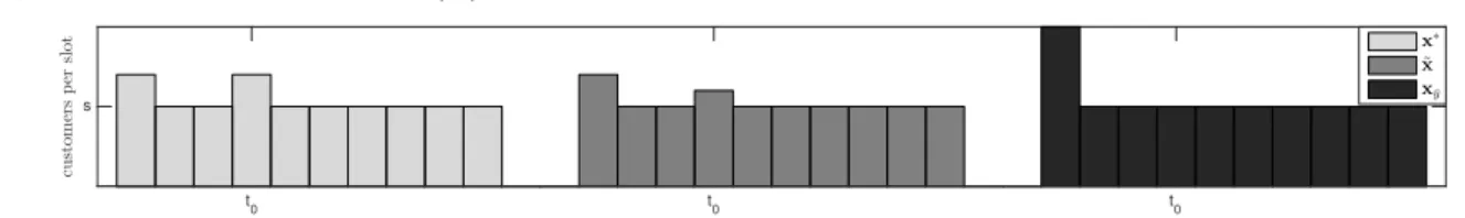
In other words, we consider schedules that demonstrate a periodic spike of size y0 every n0 slots, see Figure 1.
Periodic schedules give a renewal flavor to our arrival process, rendering our transient queue tractable. If we focus only on the queue length at the beginning of time slotst1, t2, ..., tN0+1, where
Figure 1 A schedule with periodic overbooking.
t(slot index)
xt
(c
u
st
om
er
s
p
er
sl
ot
)s+y 0
s
t1 t2 t3 . . .
and overtime. Consider the discrete-time bulk queueing system that evolves according to (1), with Ai being independent and identically distributed as A∼Binomial (m0, p), i= 1,2, ..., N0. In the
queueing literature such a system is referred to as a discreteDA/D/sn
0 queue. As in Janssen and
van Leeuwaarden (2005), the expected queue length right before the beginning of segment ti is
given explicitly, not recursively, by Spitzer’s identity (see Spitzer (1956)) as
E(Zti) = i−1
X
τ=1 1
τE[max(0, Yτ)]
=
i−1
X
τ=1 1
τ [E[Yτ] +E[max(0,−Yτ)]]
=
i−1
X
τ=1 1 τ
"
pτ m0−τ sn0+
τ sn0
X
k=0
(τ n0s−k)f(k;τ m0, p)
#
= (i−1)(pm0−sn0) +
i−1
X
τ=1 1 τ
τ sn0
X
k=0
(τ sn0−k)f(k;τ m0, p), (10)
whereYτ=
Pτ
i=1(Ai−s) denotes theτ-fold convolution of (A−s). The expected system’s overtime and idle time can now be expressed as
O(xn0,y0) =E(ZtN
0+1) =pm0N0
−sn0N0+
N0
X
τ=1 1 τ
τ sn0
X
k=0
(τ sn0−k)f(k;τ m0, p), (11)
and I(xn0,y0) =O(xn0,y0) +sn0N0−pm0N0=
N0
X
τ=1 1 τ
τ sn0
X
k=0
(τ sn0−k)f(k;τ m0, p). (12)
Note that (7) and (8) are special cases of (11) and (12) respectively whenn0=n.
Theorem 2. (i) I(xn0,y0) is decreasing and discretely convex iny0 on {0,1, ...}. (ii) O(xn0,y0) is increasing and discretely convex iny0 on {0,1, ...}.
Periodic schedules, besides being analytically tractable, turn out to yield computationally inex-pensive and very well performing heuristic solutions. Algorithm 1 describes the Periodic Overbook-ing Heuristic (POH) in terms of solvOverbook-ing n convex programs. As demonstrated in §4, the middle segment of the optimal schedule often has the pattern of one of the following three special cases: (a) y0= 1 for somen0>1 corresponding to moderate overbooking,
(b) n0= 1 corresponding to frequent overbooking when no-show rates are high, (c) n0=n when it is optimal to overbook only at the beginning of the schedule.
Algorithm 1 Periodic Overbooking Heuristic (POH) 1: procedurePOH(n, s, w, q, cO)
2: xPOH←sen .initiation state - no overbooking,enis the vector ofnone’s,
3: costPOH←(1−p)ns .only idle time cost
4: forn0= 1,2, ..., ndo
5: y0∗←arg miny0[I(xn0,y0) +c0O(xn0,y0)] .discrete convex program
6: l←n mod n0
7: x←(xn0,y∗
0;sel) .elis the vector oflone’s
8: cost←[I(x) +c0O(x) +wW(x)] 9: if cost<costPOH then
10: xPOH←x
11: costPOH←cost
12: end if
13: end for
14: return xPOH and costPOH 15: end procedure
3.5. Front-Loading Heuristic
The overbooking level y∗ contains much of the information regarding the optimal schedules. As demonstrated in the following section, the overbooked customers are allocated according to a front-loadedpattern: more customers are scheduled towards the beginning of the working day (in order to get an empty system running), and towards the end of the working day the a schedule becomes less dense (in order to avoid high overtime costs).
We propose a second heuristic, the Front-Loading Heuristic (FLH), which predicts the optimal overbooking level based on our numerical analysis in §4.2, and allocates the overbooked customers in a front-loaded manner. Algorithm 2 (see Appendix) describes in detail the FLH procedure. In
§4.3 we compare the two heuristic solutions and evaluate their performance.
4. Numerical Experiments
In this section we display and discuss the results of our numerical experiments. Our analysis reveals further properties and patterns that appear in the optimal schedules, and provide us with additional insights into their overall structure. Throughout our numerical analysis, following the literature (see for example Robinson and Chen (2010, 2011), Zacharias and Pinedo (2014)), we consider an overtime cost coefficient cO= 1.5 and values of the waiting cost coefficientw between 0 and 0.60. Provider’s idleness costs more than customer’s waits, but it is less costly than provider’s overtime. We interpret that values of w between 0 and 0.10 correspond to an efficiency regime, values of w above 0.20 correspond to a quality regime, and between 0.10 and 0.20 to a hybrid quality and
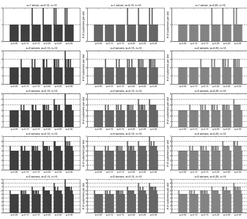
Figure 2 Optimal schedules.n= 10,s∈ {1,2,3,4,5},w∈ {0.10,0.15,0.20},q∈ {0.05,0.10,0.15,0.20,0.25,0.30}.
q=0.05 q=0.10 q=0.15 q=0.20 q=0.25 q=0.30
0 1 2
# of customers per slot
s=1 server, w=0.10, n=10
q=0.05 q=0.10 q=0.15 q=0.20 q=0.25 q=0.30
0 1 2
# of customers per slot
s=1 server, w=0.15, n=10
q=0.05 q=0.10 q=0.15 q=0.20 q=0.25 q=0.30
0 1 2
# of customers per slot
s=1 server, w=0.20, n=10
q=0.05 q=0.10 q=0.15 q=0.20 q=0.25 q=0.30
0 1 2 3 4
# of customers per slot
s=2 servers, w=0.10, n=10
q=0.05 q=0.10 q=0.15 q=0.20 q=0.25 q=0.30
0 1 2 3 4
# of customers per slot
s=2 servers, w=0.15, n=10
q=0.05 q=0.10 q=0.15 q=0.20 q=0.25 q=0.30
0 1 2 3 4
# of customers per slot
s=2 servers, w=0.20, n=10
q=0.05 q=0.10 q=0.15 q=0.20 q=0.25 q=0.30 0 1 2 3 4 5 6
# of customers per slot
s=3 servers, w=0.10, n=10
q=0.05 q=0.10 q=0.15 q=0.20 q=0.25 q=0.30 0 1 2 3 4 5 6
# of customers per slot
s=3 servers, w=0.15, n=10
q=0.05 q=0.10 q=0.15 q=0.20 q=0.25 q=0.30 0 1 2 3 4 5 6
# of customers per slot
s=3 servers, w=0.20, n=10
q=0.05 q=0.10 q=0.15 q=0.20 q=0.25 q=0.30 0 1 2 3 4 5 6 7
# of customers per slot
s=4 servers, w=0.10, n=10
q=0.05 q=0.10 q=0.15 q=0.20 q=0.25 q=0.30 0 1 2 3 4 5 6 7
# of customers per slot
s=4 servers, w=0.15, n=10
q=0.05 q=0.10 q=0.15 q=0.20 q=0.25 q=0.30 0 1 2 3 4 5 6 7
# of customers per slot
s=4 servers, w=0.20, n=10
q=0.05 q=0.10 q=0.15 q=0.20 q=0.25 q=0.30 0 1 2 3 4 5 6 7 8 9
# of customers per slot
s=5 servers, w=0.10, n=10
q=0.05 q=0.10 q=0.15 q=0.20 q=0.25 q=0.30 0 1 2 3 4 5 6 7 8 9
# of customers per slot
s=5 servers, w=0.15, n=10
q=0.05 q=0.10 q=0.15 q=0.20 q=0.25 q=0.30 0 1 2 3 4 5 6 7 8 9
# of customers per slot
s=5 servers, w=0.20, n=10
efficiency regime. Whenever we find it necessary, all the quantities of interest are subscripted by s, the number of servers.
4.1. Optimal Schedules
Optimal schedules are displayed in Figure 2 for different no-show rates q, different waiting cost coefficients w, and for up to 5 servers. It is evident, and intuitive, that the optimal overbooking
levely∗=m∗−nsis increasing inq. Aswincreases, the optimal schedules become less front-loaded,
without necessarily observing a decrease in the overbooking level. Further, many optimal schedules exhibit a “spike” at the first appointment slot, in agreement with the seminal results of Bailey (1952) and Welch and Bailey (1952) for the single server case. The overbooking level increases significantly with the number of parallel servers, and that increase is more prevalent for higher no-show rates.
Recall that in §3.3 we established that the solution to a discretely convex optimization problem (the scheduling problem wherew= 0) provides an upper bound for the optimal overbooking level y∗. In Table 1 we demonstrate that this upper bound is often tight. Consider for example the
case where q = 20% and s= 2 servers. The optimal solution to (P2) is (6,2,2,2,2,2,2,2,2,2) with an overbooking level of 4 customers. The optimal solution to (P1) for w= 0.05 has the same overbooking level, but the actual schedule (4,2,3,2,3,2,2,2,2,2) looks quite different. The overbooked customers are spread out more uniformly over the working day with a moderate “spike” at the first slot.
Table 1 Optimal schedules and overbooking levels.n= 10,s∈ {1,2,3},w∈ {0.00,0.05,0.10,0.15},
q∈ {0.05,0.10,0.15,0.20,0.25,0.30}.
s= 1 s= 2 s= 3
q= 0.05
w= 0.00 x∗= 1 1 1 1 1 1 1 1 1 1 y∗= 0 x∗= 3 2 2 2 2 2 2 2 2 2 y∗= 1 x∗=14 3 3 3 3 3 3 3 3 3 y∗=11 w= 0.05 x∗= 1 1 1 1 1 1 1 1 1 1 y∗= 0 x∗= 2 2 2 2 2 2 2 2 2 2 y∗= 0 x∗=14 3 3 3 3 3 3 3 3 3 y∗=11 w= 0.10 x∗= 1 1 1 1 1 1 1 1 1 1 y∗= 0 x∗= 2 2 2 2 2 2 2 2 2 2 y∗= 0 x∗=13 3 3 3 3 3 3 3 3 3 y∗=10 w= 0.15 x∗= 1 1 1 1 1 1 1 1 1 1 y∗= 0 x∗= 2 2 2 2 2 2 2 2 2 2 y∗= 0 x∗=13 3 3 3 3 3 3 3 3 3 y∗=10
q= 0.10
w= 0.00 x∗= 2 1 1 1 1 1 1 1 1 1 y∗= 1 x∗= 4 2 2 2 2 2 2 2 2 2 y∗= 2 x∗=16 3 3 3 3 3 3 3 3 3 y∗=13 w= 0.05 x∗= 1 1 1 1 1 1 1 1 1 1 y∗= 0 x∗= 3 2 2 2 2 2 2 2 2 2 y∗= 1 x∗=14 3 4 3 3 3 3 3 3 3 y∗=12 w= 0.10 x∗= 1 1 1 1 1 1 1 1 1 1 y∗= 0 x∗= 3 2 2 2 2 2 2 2 2 2 y∗= 1 x∗=14 3 3 4 3 3 3 3 3 3 y∗=12 w= 0.15 x∗= 1 1 1 1 1 1 1 1 1 1 y∗= 0 x∗= 3 2 2 2 2 2 2 2 2 2 y∗= 1 x∗=14 3 3 4 3 3 3 3 3 3 y∗=12
q= 0.15
w= 0.00 x∗= 2 1 1 1 1 1 1 1 1 1 y∗= 1 x∗= 5 2 2 2 2 2 2 2 2 2 y∗= 3 x∗=17 3 3 3 3 3 3 3 3 3 y∗=14 w= 0.05 x∗= 2 1 1 1 1 1 1 1 1 1 y∗= 1 x∗= 3 2 3 2 2 2 2 2 2 2 y∗= 2 x∗=15 3 4 3 4 3 3 3 3 3 y∗=14 w= 0.10 x∗= 2 1 1 1 1 1 1 1 1 1 y∗= 1 x∗= 3 2 2 3 2 2 2 2 2 2 y∗= 2 x∗=14 4 3 3 4 3 3 3 3 3 y∗=13 w= 0.15 x∗= 1 1 1 1 1 1 1 1 1 1 y∗= 0 x∗= 3 2 2 3 2 2 2 2 2 2 y∗= 2 x∗=14 3 4 3 3 4 3 3 3 3 y∗=13
q= 0.20
w= 0.00 x∗= 3 1 1 1 1 1 1 1 1 1 y∗= 2 x∗= 6 2 2 2 2 2 2 2 2 2 y∗= 4 x∗=19 3 3 3 3 3 3 3 3 3 y∗=16 w= 0.05 x∗= 2 1 1 1 1 1 1 1 1 1 y∗= 1 x∗= 4 2 3 2 3 2 2 2 2 2 y∗= 4 x∗=15 4 4 3 4 3 4 3 3 3 y∗=16 w= 0.10 x∗= 2 1 1 1 1 1 1 1 1 1 y∗= 1 x∗= 3 3 2 2 3 2 2 2 2 2 y∗= 3 x∗=14 4 4 3 4 3 4 3 3 3 y∗=15 w= 0.15 x∗= 2 1 1 1 1 1 1 1 1 1 y∗= 1 x∗= 3 2 3 2 2 3 2 2 2 2 y∗= 3 x∗=14 4 4 3 4 3 4 3 3 3 y∗=15
q= 0.25
w= 0.00 x∗= 4 1 1 1 1 1 1 1 1 1 y∗= 3 x∗= 8 2 2 2 2 2 2 2 2 2 y∗= 6 x∗= 12 3 3 3 3 3 3 3 3 3 y∗=19 w= 0.05 x∗= 2 1 2 1 1 1 1 1 1 1 y∗= 2 x∗= 4 3 2 3 2 3 2 2 2 2 y∗= 5 x∗=15 4 4 4 4 4 4 3 3 3 y∗=18 w= 0.10 x∗= 2 1 2 1 1 1 1 1 1 1 y∗= 2 x∗= 3 3 2 3 2 3 2 2 2 2 y∗= 4 x∗=15 4 4 4 3 4 4 3 3 3 y∗=17 w= 0.15 x∗= 2 1 1 1 1 1 1 1 1 1 y∗= 1 x∗= 3 3 2 3 2 3 2 2 2 2 y∗= 4 x∗=15 4 3 4 4 4 3 4 3 3 y∗=17
q= 0.30
w= 0.00 x∗= 4 1 1 1 1 1 1 1 1 1 y∗= 3 x∗= 9 2 2 2 2 2 2 2 2 2 y∗= 7 x∗= 14 3 3 3 3 3 3 3 3 3 y∗= 11 w= 0.05 x∗= 2 2 1 2 1 1 1 1 1 1 y∗= 3 x∗= 4 3 3 3 3 2 3 2 2 2 y∗= 7 x∗=16 5 4 4 4 4 4 4 3 3 y∗= 11 w= 0.10 x∗= 2 1 2 1 1 1 1 1 1 1 y∗= 2 x∗= 4 3 2 3 3 2 3 2 2 2 y∗= 6 x∗=16 4 4 4 4 4 4 4 3 3 y∗= 10 w= 0.15 x∗= 2 1 1 2 1 1 1 1 1 1 y∗= 2 x∗= 3 3 3 2 3 2 3 2 2 2 y∗= 5 x∗=15 4 4 4 4 4 4 4 3 3 y∗=19
In Table 2 we demonstrate the effect of the number of slots non the optimal schedule. There is evidence for a linear relationship between the overbooking level andn, by observing that the cases where n= 10, 15, 20, 25, 30, 35 and 40 slots have corresponding overbooking levels y= 2, 3, 4, 5, 6, 7 and 8 respectively. Moreover, asnincreases, a periodic pattern appears in the middle segment of the schedule.
Table 2 Optimal schedules as a function ofn.s= 2,q= 0.15,w= 0.10.
n x
10 3 2 2 3 2 2 2 2 2 2
15 3 2 2 3 2 2 2 3 2 2 2 2 2 2 2
20 3 2 2 3 2 2 2 3 2 2 2 2 3 2 2 2 2 2 2 2
25 3 2 2 3 2 2 2 3 2 2 2 2 3 2 2 2 2 3 2 2 2 2 2 2 2
30 3 2 2 3 2 2 2 3 2 2 2 2 3 2 2 2 2 3 2 2 2 2 3 2 2 2 2 2 2 2
35 3 2 2 3 2 2 2 3 2 2 2 2 3 2 2 2 2 3 2 2 2 2 3 2 2 2 2 3 2 2 2 2 2 2 2
40 3 2 2 3 2 2 2 3 2 2 2 2 3 2 2 2 2 3 2 2 2 2 3 2 2 2 2 3 2 2 2 2 3 2 2 2 2 2 2 2
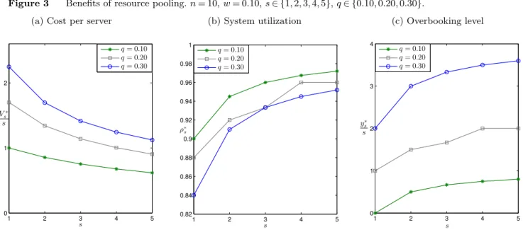
Next, we focus on the system performance as a function of the number of servers s and the no-show rate q. Let ρ∗
s= pm∗
ns be the system’s utilization under the optimal schedule. The benefits
of resource pooling are apparent in two dimensions: (a) decreasing the total cost (V
∗
s
s decreasing
in s), (b) increasing the system’s utilization (ρ∗
s increasing in s), and consequently increasing the
customers’ access to services (y
∗
s
s increasing in s). These gains are illustrated in Figure 3. We also
observe that higher no-show rates come along with a more costly system, since both waiting times and system’s idleness increase with the variability in the arrival process.
Figure 3 Benefits of resource pooling.n= 10,w= 0.10,s∈ {1,2,3,4,5},q∈ {0.10,0.20,0.30}. (a) Cost per server
1 2 3 4 5
0 1 2
s
q= 0.10
q= 0.20
q= 0.30
V∗
s s
(b) System utilization
1 2 3 4 5
0.82 0.84 0.86 0.88 0.9 0.92 0.94 0.96 0.98 1
s
q= 0.10
q= 0.20
q= 0.30
ρ∗s
(c) Overbooking level
1 2 3 4 5
0 1 2 3 4
s q= 0.10 q= 0.20 q= 0.30
y∗s s
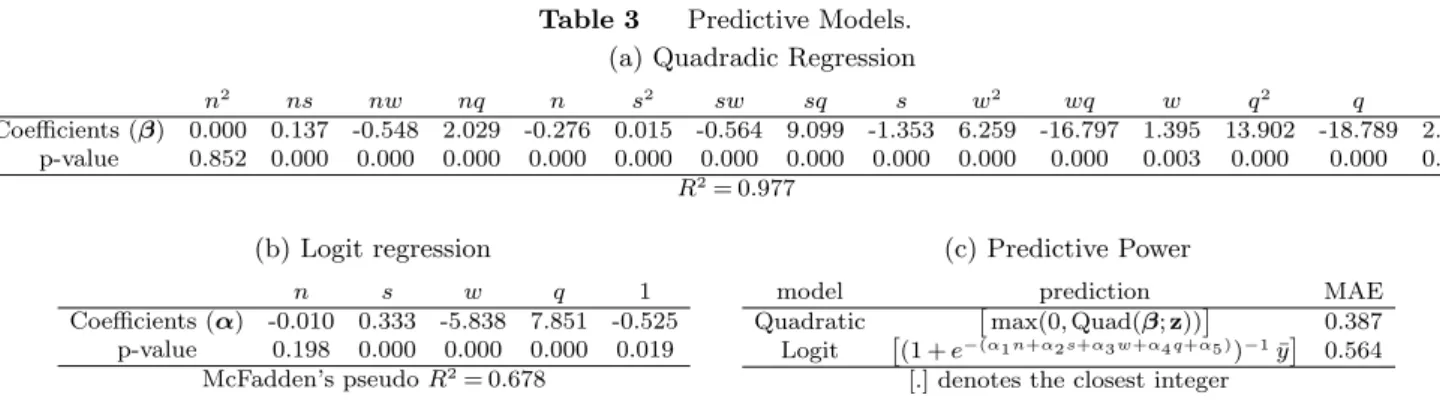
4.2. Predictive Models for the Optimal Overbooking Level
The overbooking level y∗ contains much of the information regarding the optimal schedules. In this section we employ predictive models to predicty∗ as a function of the independent variables n,s,w, andq. An equivalent way to capture y∗ is through the proportion yp=y
∗
¯
y, where ¯y is the
upper bound derived in§3.3. We use the Logit model to predict the proportionyp, and Quadratic
In the Logit model the expected value for the proportion yp given the system’s parameters z= (n, s, w, q) is
E(yp|z) = (1 +e−(β1n+β2s+β3w+β4q+β5))−1, (13)
for some coefficient vectorβ= (β1, ..., β5).
The more elaborate Quadratic regression is a form of linear regression in which the relationship betweeny∗ and z is modeled as a second-order polynomial
E(y∗|z) =Quad(β;z)
,β1n2+β2ns+β3nw+β4nq+β5n+β6s2+β7sw+β8sq
+β9s+β10w2+β11wq+β12w+β13q2+β14q+β15.
(14)
Our data set was generated by solving 4500 instances of the optimization problem (P1). For the solved instances the length of the working day n takes values in {5,6, ...,32} and we consider problems with up tos= 10 servers. The waiting cost coefficientwtakes values in{0,0.05, ...,0.60}, and the no-show rateq in{0.05,0.10, ...,0.40}. The idle time cost coefficient cI is normalized to 1 and the overtime cost coefficient is fixed at cO= 1.5. The maximum observed overbooking level is 31 customers. Randomly chosen, two thirds of the instances are used as our training set, and the rest as our test set.
Though we could have considered higher-order polynomials, a quadratic regression fits our train-ing data well, yieldtrain-ing a 0.98 R-squared. We evaluate the goodness-of-fit of our Logit model with the McFadden pseudo R-squared, as proposed by McFadden (1974). A 0.68 pseudo R-squared indicates a very good explanation of our training data.
Table 3 Predictive Models. (a) Quadradic Regression
n2 ns nw nq n s2 sw sq s w2 wq w q2 q 1
Coefficients (β) 0.000 0.137 -0.548 2.029 -0.276 0.015 -0.564 9.099 -1.353 6.259 -16.797 1.395 13.902 -18.789 2.256 p-value 0.852 0.000 0.000 0.000 0.000 0.000 0.000 0.000 0.000 0.000 0.000 0.003 0.000 0.000 0.000
R2= 0.977
(b) Logit regression
n s w q 1
Coefficients (α) -0.010 0.333 -5.838 7.851 -0.525 p-value 0.198 0.000 0.000 0.000 0.019
McFadden’s pseudoR2= 0.678
(c) Predictive Power
model prediction MAE
Quadratic
max(0,Quad(β;z))
0.387 Logit
(1 +e−(α1n+α2s+α3w+α4q+α5 ))−1¯y
0.564 [.] denotes the closest integer
The results of the two regressions are summarized in Table 3 (a) and (b). The only statistically non-significant variable (at level 0.05) in the Quadratic model for predictingy∗ is the square of the
number of slotsn, confirming our observations of a linear relationship in §4.1. Regarding the Logit model for the proportionyp, the number of slotsnis the only non-significant variable. Interestingly
though, its coefficient is negative, indicating that the larger the length of the working day, the less likely it is that the overbooking level achieves its upper bound.
Finally, we evaluate the predictive power of the two models via theMean Absolute Error (MAE)
over the test set. The predictions are made as in Table 3 (c). The proportion yp, estimated by
the Logit model, is multiplied with the upper bound ¯y and rounded to the closest integer. The Quadratic model is further corrected for negative values, which are mapped to zero-overbooking level. Both models perform very well, with MAE’s less than 0.6. The Quadratic model makes the most accurate predictions yielding the smallest MAE at 0.387.
Building upon our prediction for the optimal overbooking level, we propose the Front Loading Heuristic (FLH). In particular, given the system’s parametersn,s,wandq, we overbook a number of customers as suggested by the quadratic model, in agreement with the front-loaded pattern observed in§4.1. Algorithm 2 (appearing in the Appendix) describes in detail the FLH procedure.
4.3. Evaluation of POH and FLH
Finally, we evaluate the performances of POH and FLH via their cost difference relative to the optimal schedules. The comparison is based on all 4500 instances described in§4.2. Both POH and FLH yield very well performing schedules, with the average cost difference being 5.09% and 3.49% respectively. We display in Table 4 a sample comparison for a working day consisting of n= 16 slots (for example an 8-hour working day with slots of 30 min length) and for different values of s, w, q.
A solution to a convex program provides the overbooking level in the POH. On the other hand, FLH overbooks a number of customers as suggested by our predictive models in §4.2. Periodic schedules, besides being analytically tractable, turn out to provide very well performing and com-putationally inexpensive heuristic solutions. In most of the cases POH provides the optimal over-booking level, but, due to its periodic nature, the allocation of the overbooked customers is not the optimal one. Only trivial cases, where all the overbooking occurs at the first slot, are solved to optimality. FLH, on the other hand, often provides schedules identical to the optimal one for non-trivial cases as well (see Table 4). Even though on average FLH performs better than POH, it is not clear under what circumstances in general which heuristic is better than the other.
5. Heterogeneous Customers
Consider now the more general model where customers are heterogeneous in two dimensions: they have different waiting cost coefficients and different no-show rates, reflecting their type and their history in attending scheduled appointments respectively. The scheduler would like to assign each one of the customers to arrive at the beginning of one of the time slots. Customer j,j= 1, . . . , m,
Table 4 Performance of POH and FLH compared to the optimal schedules.n= 16,s∈ {1,2,3},
w∈ {0.05,0.10,0.15},q∈ {0.10,0.15,0.20}.
s= 1 s= 2 s= 3
q = 0 . 10 w = 0 .
05 ( 2 1 1 1 1 1 1 1 1 1 1 1 1 1 1 1 ) ( 3 2 2 2 3 2 2 2 2 2 2 2 2 2 2 2 ) ( 4 4 3 3 4 3 3 3 4 3 3 3 3 3 3 3 )
[ 2 1 1 1 1 1 1 1 1 1 1 1 1 1 1 1 ] [ 3 2 2 2 2 2 3 2 2 2 2 2 2 2 2 2 ] [ 5 3 3 3 3 3 5 3 3 3 3 3 3 3 3 3 ]
{2 1 1 1 1 1 1 1 1 1 1 1 1 1 1 1} {3 2 2 2 2 2 2 3 2 2 2 2 2 2 2 2} {4 3 3 4 3 3 3 4 3 3 3 4 3 3 3 3}
∗0.00% ∗∗0.00% ∗1.23% ∗∗2.72% ∗4.17% ∗∗6.04%
w
=
0
.
10 ( 1 1 1 1 1 1 1 1 1 1 1 1 1 1 1 1 ) ( 3 2 2 2 2 3 2 2 2 2 2 2 2 2 2 2 ) ( 4 3 3 4 3 3 3 3 4 3 3 3 3 3 3 3 )
[ 1 1 1 1 1 1 1 1 1 1 1 1 1 1 1 1 ] [ 3 2 2 2 2 2 3 2 2 2 2 2 2 2 2 2 ] [ 4 3 3 3 3 4 3 3 3 3 4 3 3 3 3 3 ]
{1 1 1 1 1 1 1 1 1 1 1 1 1 1 1 1} {3 2 2 2 2 2 2 3 2 2 2 2 2 2 2 2} {4 3 3 4 3 3 3 4 3 3 3 4 3 3 3 3}
∗0.00% ∗∗0.00% ∗0.13% ∗∗0.83% ∗2.63% ∗∗6.94%
w
=
0
.
15 ( 1 1 1 1 1 1 1 1 1 1 1 1 1 1 1 1 ) ( 3 2 2 2 2 2 2 2 2 2 2 2 2 2 2 2 ) ( 4 3 3 3 4 3 3 3 3 4 3 3 3 3 3 3 )
[ 1 1 1 1 1 1 1 1 1 1 1 1 1 1 1 1 ] [ 3 2 2 2 2 2 2 2 2 2 2 2 2 2 2 2 ] [ 4 3 3 3 3 4 3 3 3 3 4 3 3 3 3 3 ]
{1 1 1 1 1 1 1 1 1 1 1 1 1 1 1 1} {3 2 2 2 2 2 2 2 2 2 2 2 2 2 2 2} {4 3 3 3 4 3 3 3 3 4 3 3 3 3 3 3}
∗0.00% ∗∗0.00% ∗0.00% ∗∗0.00% ∗1.10% ∗∗0.00%
q = 0 . 15 w = 0 .
05 ( 2 1 1 1 1 1 1 1 1 1 1 1 1 1 1 1 ) ( 3 3 2 2 3 2 2 2 3 2 2 2 2 2 2 2 ) ( 4 4 3 4 3 4 3 4 3 3 4 3 3 3 3 3 )
[ 2 1 1 1 1 1 1 1 1 1 1 1 1 1 1 1 ] [ 4 2 2 2 2 2 4 2 2 2 2 2 2 2 2 2 ] [ 6 3 3 3 3 3 6 3 3 3 3 3 3 3 3 3 ]
{2 1 1 1 1 1 1 2 1 1 1 1 1 1 1 1} {3 2 2 3 2 2 2 3 2 2 2 3 2 2 2 2} {4 4 3 4 3 4 3 4 3 4 3 3 3 3 3 3}
∗0.00% ∗∗4.05% ∗3.87% ∗∗6.09% ∗6.24% ∗∗0.17%
w
=
0
.
10 ( 2 1 1 1 1 1 1 1 1 1 1 1 1 1 1 1 ) ( 3 2 2 3 2 2 2 2 3 2 2 2 2 2 2 2 ) ( 4 4 3 4 3 4 3 3 4 3 3 4 3 3 3 3 )
[ 2 1 1 1 1 1 1 1 1 1 1 1 1 1 1 1 ] [ 3 2 2 2 2 3 2 2 2 2 3 2 2 2 2 2 ] [ 4 3 3 4 3 3 4 3 3 4 3 3 4 3 3 3 ]
{2 1 1 1 1 1 1 1 1 1 1 1 1 1 1 1} {3 2 2 3 2 2 2 3 2 2 2 3 2 2 2 2} {4 4 3 4 3 4 3 4 3 4 3 3 3 3 3 3}
∗0.00% ∗∗0.00% ∗2.55% ∗∗4.73% ∗4.85% ∗∗1.17%
w
=
0
.
15 ( 2 1 1 1 1 1 1 1 1 1 1 1 1 1 1 1 ) ( 3 2 2 3 2 2 2 2 3 2 2 2 2 2 2 2 ) ( 4 3 4 3 3 4 3 3 4 3 3 4 3 3 3 3 )
[ 2 1 1 1 1 1 1 1 1 1 1 1 1 1 1 1 ] [ 3 2 2 2 2 3 2 2 2 2 3 2 2 2 2 2 ] [ 4 3 3 4 3 3 4 3 3 4 3 3 4 3 3 3 ]
{2 1 1 1 1 1 1 1 1 1 1 1 1 1 1 1} {3 2 2 2 3 2 2 2 2 3 2 2 2 2 2 2} {4 3 4 3 3 4 3 3 4 3 3 4 3 3 3 3}
∗0.00% ∗∗0.00% ∗1.18% ∗∗0.07% ∗2.06% ∗∗0.00%
q = 0 . 20 w = 0 .
05 ( 2 1 1 1 2 1 1 1 1 1 1 1 1 1 1 1 ) ( 4 2 3 2 3 2 2 3 2 2 3 2 2 2 2 2 ) ( 5 4 4 4 3 4 4 3 4 3 4 3 4 3 3 3 )
[ 2 1 1 1 1 1 2 1 1 1 1 1 1 1 1 1 ] [ 5 2 2 2 2 2 2 5 2 2 2 2 2 2 2 2 ] [ 6 3 3 3 3 6 3 3 3 3 6 3 3 3 3 3 ]
{2 1 1 1 2 1 1 1 1 2 1 1 1 1 1 1} {3 3 2 3 2 3 2 3 2 3 2 2 2 2 2 2} {5 4 4 4 3 4 3 4 3 4 3 4 3 3 3 3}
∗1.17% ∗∗5.59% ∗7.92% ∗∗0.48% ∗10.50% ∗∗0.26%
w
=
0
.
10 ( 2 1 1 1 1 2 1 1 1 1 1 1 1 1 1 1 ) ( 3 3 2 2 3 2 2 3 2 2 3 2 2 2 2 2 ) ( 5 3 4 4 3 4 4 3 4 3 4 3 4 3 3 3 )
[ 2 1 1 1 1 1 2 1 1 1 1 1 1 1 1 1 ] [ 3 2 2 3 2 2 3 2 2 3 2 2 3 2 2 2 ] [ 4 3 4 3 4 3 4 3 4 3 4 3 4 3 4 3 ]
{2 1 1 1 2 1 1 1 1 2 1 1 1 1 1 1} {3 2 3 2 2 3 2 2 3 2 2 3 2 2 2 2} {4 4 3 4 3 4 3 4 3 4 3 4 3 4 3 3}
∗0.21% ∗∗11.72% ∗4.39% ∗∗1.05% ∗10.09% ∗∗2.93%
w
=
0
.
15 ( 2 1 1 1 1 1 1 1 1 1 1 1 1 1 1 1 ) ( 3 2 3 2 2 3 2 2 3 2 2 3 2 2 2 2 ) ( 4 4 4 3 4 3 4 3 4 3 4 3 4 3 3 3 )
[ 2 1 1 1 1 1 2 1 1 1 1 1 1 1 1 1 ] [ 3 2 2 3 2 2 3 2 2 3 2 2 3 2 2 2 ] [ 4 3 4 3 4 3 4 3 4 3 4 3 4 3 4 3 ]
{2 1 1 1 1 1 1 2 1 1 1 1 1 1 1 1} {3 2 3 2 2 3 2 2 3 2 2 3 2 2 2 2} {4 4 3 4 3 4 3 4 3 4 3 4 3 3 3 3}
∗1.50% ∗∗1.74% ∗2.16% ∗∗0.00% ∗6.62% ∗∗1.31%
(.) denotesx∗, [.] denotesx
POH,{.}denotesxFLH,
∗denotes the POH cost difference,∗∗denotes the FLH cost difference
will show up with probabilitypj= 1−qj∈(0,1) at the beginning of the time slot she was assigned,
has a waiting cost coefficient wj, and requires one time slot of service. LetC={1,2, ..., m} denote
the set of all customers to be scheduled.
A schedule is defined as a pair of vectors (σ,x), where σ= (σ1, σ2, ..., σm) is a permutation of C, and x= (x1, x2, ..., xn) is such that xt customers are assigned to slot t, with
Pn
t=1xt=m, and customers (σ1, σ2, ..., σx1) are assigned to slot 1, customers (σx1+1, σx1+2, ..., σx1+x2) are assigned
to slot 2, and so on. For better presentation of our analysis, let st=
Pt
τ=1xτ be the sum of all customers scheduled up to slott, 1≤t≤n. As a convention,s0= 0.
Let I(σ,x) and O(σ,x) denote the expected total servers’ idle time and overtime associated with schedule (σ,x) respectively. Note that
and therefore
I(σ,x) =O(σ,x) +ns− m
X
j=1
pj. (15)
Also let Bj(σ,x) be the random variable denoting the backlog of customers that have priority
over customer j upon her arrival (if customer j shows up). Then the expected waiting time of customerj, measured in time slots, is
Wj(σ,x) =pj
X
k≥s
Pr(Bj(σ,x) =k)
k s
. (16)
The objective function is the weighted sum of servers’ expected idle time, overtime, and cus-tomers’ waiting time
V(σ,x) =cII(σ,x) +cOO(σ,x) +
m
X
j=1
wjWj(σ,x), (17)
and we consider the optimization problem (P4) min
(σ,x) V(σ,x)
s.t. σis a permutation ofC,
xtis a nonnegative integer for t= 1,2, ..., n, n
X
t=1
xt=m.
(P4)
Theorem 3 characterizes an optimal solution to (P4) in terms of a priority rule and a sequencing rule. In order to display the latter, let ˜Btbe the random variable denoting the number of customers
among (σ1, σ2, ..., σst−1) still present at the beginning of slot t, i.e., the backlog of customers that
have priority over customerσst, 1≤t≤n.
Theorem 3. An optimal schedule(σ∗,x∗) satisfies the following properties:
(i) The customers assigned to each one of the slots 1, . . . , n are prioritized in decreasing order of their weight wj.
(ii) For t∈
τ: 1≤τ≤n−1, x∗τ+1=s , for j=σ
∗
st and k=σ ∗
st+1, the following sequencing rule holds:
pjwj
Pr( ˜Bt≥s)−Pr( ˜Bt= (s−1)mod s,B˜t≥s)pj
≤ pkwk
Pr( ˜Bt≥s)−Pr( ˜Bt= (s−1)mod s,B˜t≥s)pk . (18)
The following corollary is a direct consequence of Theorem 3. It demonstrates simplified expres-sions of the sequencing rule in (18) with intuitive interpretations for four special case.
Corollary 1. (i) If m−ns < s, then the sequencing rule in Theorem 3 becomes pjwj≤pkwk.
(ii) If pj=p for all j∈ C, then the sequencing rule in Theorem 3 becomes wj≤wk.
(iv) If s= 1, then the sequencing rule in Theorem 3 becomes pjwj
1−pj ≤ pkwk
1−pk.
As suggested by (i) and (ii) of Corollary 1, customers with larger weights tend to be scheduled at slots where they are expected to encounter a shorter queue and therefore incur smaller waiting costs. From (iii) of Corollary 1, customers between consecutive overbooked slots are sequenced in decreasing order of their no-show probability: the further away a customer is assigned from an overbooked slot, the more likely she is to show up and to encounter a shorter queue. As a remark, the sequencing rule in (iv) of Corollary 1 is theSmallest Weighted Probability of Showing Up first rule that appears in Zacharias and Pinedo (2014), where they analyze a single server model.
6. Conclusion
To the best of our knowledge, this is the first study to develop and analyze a stylized appoint-ment scheduling model for managing customer arrivals in a service system with more than one server. Theoretical and heuristic guidelines are provided for the effective practice of appointment overbooking to offset no-shows.
When customers come from a homogeneous pool, recursive expressions for the performance measures of interest are derived and we provide an upper bound for the optimal overbooking level. Our extensive numerical experiments reveal further properties and patterns that appear in the optimal schedules, and motivate the development of two very well performing and computationally inexpensive heuristic solutions. Periodic schedules have a simple form, are analytically tractable, and yield solutions on average 5.1% more costly than the optimal ones. Our front loading heuristic predicts quite accurately the optimal overbooking level, often provides a solution identical to the optimal one, and has an average cost difference of 3.5%. For the case of heterogeneous customers, we provide structural properties of an optimal schedule and we introduce a new sequencing rule.
For the sake of analytical tractability, and in order to focus specifically on the uncertainty resulting from no-shows, we did not model the variability in service times. Deterministic service times, however, have been considered in the literature (e.g. Green and Savin (2008), LaGanga and Lawrence (2007), Zacharias and Pinedo (2014)) and have shown to yield useful approximations and insights. Customer non-punctuality is not captured by our model. As discussed in§2, appoint-ment scheduling models become intractable if multiple features are considered simultaneously, and typically transient analysis of rich queueing systems is addressed either via computer simulation or approximations (for example diffusion processes).
An interesting future research direction is to account for non-perfectly pooled service providers. In practice, situations often arise where a stream of customers is dedicated to a particular provider (for example in a group physician practice), whereas some other customers do not have a preference and go to the next available provider.
Acknowledgments
The authors gratefully acknowledge the support of the Alexander S. Onassis Foundation.
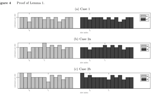
Appendix
Proof of Lemma 1 Assumex= (x1, x2, ..., xn) is a schedule with at least one slot with less than
scustomers assigned to it, and tett0be the first such slot, i.e.,t0= min{t:xt< s}. Letm=
Pn
t=1xt.
We will show via contradiction that xcannot be optimal.
Case 1: Assume xt≤sfor allt=6 t0. Then Pr(At≤s) = 1 for all t= 1,2, ..., n+ 1, and therefore,
from (1), Pr(Zt= 0) = 1 for allt= 1,2, ..., n+ 1. From (4), (5) and (6) we get
O(x) = 0
I(x) =ns−mp >0 (19) W(x) = 0.
Consider now the schedule (see Figure 4)
x0= (x1, x2, ..., xt0−1, xt0+ 1, xt0+1, ..., xt1−1, xt1−1, xt1+1, ..., xn)
and letA0
tandZt0 be the associated new arrivals and backlog at the beginning of slottrespectively.
Then
O(x0) = 0
I(x0) =ns−(m+ 1)p≥0 (20)
W(x0) = 0.
From (19) and (20), and by the assumption that p >0, schedule x0 is less costly thanx.
Case 2: Assume xt> s for for some t6=t0, i.e., there is at least one slot with more than s
customers assigned to it.
Case 2a: Suppose that the first slot with more thans customers assigned to it appears after slott0, and lett1 be that slot, i.e., t1= min{t:xt> s, t > t0}(see Figure 4). This implies that slots
1,2, . . . , t0−1 have at most scustomers assigned to each one of them. Consider now the schedule
ˆ
x= (x1, x2, ..., xt0−1, xt0+ 1, xt0+1, ..., xt1−1, xt1−1, xt1+1, ..., xn).
Then
and Pr( ˆAt1> a)<Pr(At1> a) for all a≥0, i.e., ˆAt1<stAt1. Therefore, from (1),
ˆ
Zt<stZt for allt=t1+ 1, t1+ 2, ..., n,
concluding that
O(ˆx)< O(x), I(ˆx)< I(x), and W(ˆx)< W(x).
Case 2b: Suppose that there is a slot prior to t0 with more than s customers assigned to it. Lett2be the last slot beforet0that has more thanscustomers assigned to it, i.e.,t2= max{t:xt>
s, t < t0} (see Figure 4). This implies that slotst2+ 1, . . . , t0−1 have exactly scustomers assigned to each one of them. Consider now the schedule
˜
x= (x1, x2, ..., xt2−1, xt2−1, xt2+1, ..., xt0−1, xt0+ 1, xt0+1, ..., xn).
Then ˜xt=xt and therefore
˜ Zt
d
=Zt for allt= 1,2, ..., t2. (21)
Note that ˜xt2=xt2−1 and hence Pr( ˜At2> a)<Pr(At2> a) for alla≥0, i.e., ˆAt2<stAt2. Therefore,
from (1),
˜
Zt<stZt for allt=t2+ 1, t2+ 2, ..., t0. (22)
Next, we will show that ˜Zt2+1<stZt2 for allt=t0+ 1, t0+ 2, ..., n. Since ˜xt=xt=s for all t=
t2+ 1, t2+ 2, ..., t0−1, we get that
Zt0+1= max{Zt2+ Bino ((t0−t2−1)s+xt2+xt0, p)−(t0−t2+ 1)s,0}
˜
Zt0+1= max{Z˜t2+ Bino ((t0−t2−1)s+ ˜xt2+ ˜xt0, p)−(t0−t2+ 1)s,0}.
Since ˜Zt2
d
=Zt2 and ˜xt2+ ˜xt0=xt2+xt0, we conclude that
˜ Zt
d
=Zt for allt=t0+ 1, t0+ 2, ..., n. (23)
From (21), (22) and (23) we conclude that
O(˜x)< O(x), I(˜x)< I(x), and W(˜x)< W(x).
Proof of Lemma 2 First, recall thatI(x) =O(x) +ns−mp, and therefore a schedule minimizes the expected idle if and only if it minimizes the expected overtime. It suffices to show that a schedule from class Aminimizes the total expected overtime.
Suppose that for some realization of the arrival processdout of mcustomers will actually show up. Then the total number of overtime slots must be at least max(d−ns,0), for any schedule mathbf xsuch that Pn
Figure 4 Proof of Lemma 1.
(a) Case 1
slot index t
0 t0
c u st om e rs p e r sl ot s x x′
(b) Case 2a
slot index t
0 t1 t0 t1
c u st om e rs p e r sl ot s x ˆ x
(c) Case 2b
slot index t
0 t1 t0 t1
c u st om e rs p e r sl ot s x ˜ x
Suppose a schedule belongs to class Aand that for some realization of the arrival processaout of mcustomers will actually show up. Then exactly min(a, ns) will be served during regular slots. The rest a−min(a, ns) will be served during overtime slots, and this is true for every a and for every realization of the arrival process with a arrivals. Note that a−min(a, ns) = max(0, a−ns), the minimum possible number of overtime slots. Therefore, a schedule from classA minimizes the total expected overtime and idle time.
Proof of Theorem 1 (i) It is equivalent to show that I(xy) is decreasing and discretely convex
inm=ns+y on {ns, ns+ 1, ...}. Firstly note that
I(xy+1) = ns
X
k=0
(ns−k)
m+ 1 k
pk(1−p)m+1−k
=
ns
X
k=0
(ns−k)
m k
pk(1−p)m+1−k+ ns
X
k=1
(ns−k)
m k−1
pk(1−p)m+1−k
= (1−p)
ns
X
k=0
(ns−k)
m k
pk(1−p)m−k+p
ns
X
k=1
(ns−k)
m k−1
pk−1(1−p)m−(k−1)
j=k−1
= (1−p)I(xy) +p ns−1
X
j=0
[ns−(j+ 1)]
m j
pj(1−p)m−j
= (1−p)I(xy) +p ns−1
X
j=0
(ns−j)
m j
pj(1−p)m−j−p
ns−1 X j=0 m j
pj(1−p)m−j
= (1−p)I(xy) +p ns
X
j=0
(ns−j)
m j
pj(1−p)m−j−p ns−1 X j=0 m j
= (1−p)I(xy) +pI(xy)−p ns−1 X j=0 m j
pj(1−p)m−j
=I(xy)−p ns−1 X j=0 m j
pj(1−p)m−j,
concluding that
−p < I(xy+1)−I(xy) =−p ns−1 X k=0 m k
pk(1−p)m−k<0. (24)
Therefore,I(xy) is decreasing inm=ns+y.
For the proof of the discrete convexity it suffices to show (from Theorem 1 of Y¨uceer (2002)) thatI(xy) has increasing differences inm on{ns, ns+ 1, ...}. LetPm=
Pns−1
k=0
m k
pk(1−p)m−k and
note that
Pm+1=
ns−1
X
k=0
m+ 1 k
pk(1−p)m+1−k
= ns−1 X j=0 m k
pk(1−p)m+1−k+ ns−1
X
k=1
m k−1
pk(1−p)m+1−k
= (1−p)
ns−1 X j=0 m k
pk(1−p)m−k+p
ns−1
X
k=1
m k−1
pk−1(1−p)m−(k−1)
j=k−1
= (1−p)Pm+p ns−2 X j=0 m j
pj(1−p)m−j
= (1−p)Pm+pPm−p
m ns−1
pns−1(1−p)m−(ns−1)
< Pm. (25)
From (24) and (25)
[I(xy+2)−I(xy+1)]−[I(xy+1)−I(xy)] =−p[Pm+1−Pm]>0,
concluding that I(xy) has increasing differences inm on {ns, ns+ 1, ...}.
(ii) Recall that O(xy) =pm−ns+I(xy), and therefore
O(xy+1)−O(xy) =p[(m+ 1)−m] + [I(xy+1)−I(xy)]
=p−pPm
=p(1−Pm) (26)
>0.
It is straightforward to verify thatO(xy) has increasing differences inm=ns+yon{ns, ns+ 1, ...}
(iii) Let ¯y be an optimal solution to (P2) and let ¯m=ns+ ¯y. Then cII(x¯y+1) +cOO(xy¯+1)≥ cII(xy¯) +cOO(x¯y), implying (from (24) and (26)) that
p((1 +cO)Pm¯ −cO)≤0, (27)
where Pm¯ =Pns−1
k=0 ¯
m k
pk(1−p)m−k¯ is the probability that the waiting time of the last customer of schedulexy¯+1 is equal to zero.
Let (y∗,x∗) and be an optimal solution to (P1) and assume, for contradiction, that y∗>y.¯ Let t0 be the last slot under schedule x∗ that has more than s customers assigned to it, i.e., t0= max{t:x∗
t> s}. This implies that slotst0+ 1, . . . , nhave exactlyscustomers assigned to each
one of them. Consider now the schedule ˜x= (x∗
1, x
∗
2, ..., x
∗ t0−1, x
∗ t0−1, x
∗
t0+1, ..., x
∗
n), refer to Figure
5. We will show thatI(˜x) +cOO(˜x) +wW(˜x)< I(x∗) +c OO(x
∗) +wW(x∗), under the assumption
that y∗>y.¯
Figure 5 Proof of Theorem 1 (iii).
slot index
t
0 t0 t0
c
u
st
om
e
rs
p
e
r
sl
ot
s
x∗ ˜
x x¯y
Clearly W(x∗)> W(˜x). It suffices to show that I(˜x) +c
OO(˜x)< I(x ∗) +c
OO(x
∗). Let u=
Pn
t=t0x˜t be the number of customers assigned to slots t0, ..., tn under schedule ˜x. Let also B
be the random variable denoting the backlog of customers at the beginning of slot t0, which is stochastically the same under both schedules ˜x and x∗, and let b be realization of B. Then, using
similar arguments as in (7), the expected overtime and idle time costs under schedules ˜x and x∗,
subscripted by b, are
Ob(x∗) =b+p(u+ 1)−(n−t0+ 1)s+
(n−t0+1)s−b X
k=0
[(n−t0+ 1)s−b−k]f(k;u+ 1, p)
Ob(˜x) =b+pu−(n−t0+ 1)s+
(n−t0+1)s−b X
k=0
[(n−t0+ 1)s−b−k]f(k;u, p)
Ib(x∗) =Ob(x∗) +ns−pm∗
Ib(˜x) =Ob(˜x) +ns−p(m∗−1).
Therefore
where
˜ P=X
y
Pr(B=b)
(n−t0+1)s−b−1 X
k=0
f(k;u, p)
is the probability that the waiting time of the last customer of schedule ˜x is equal to zero. Using similar arguments as in the proof of Lemma 2, and by the assumption that Pn
t=1x˜t=m
∗−1≥m,¯
we conclude that
˜
P < Pm¯. (29)
From (27), (28) and (29) it follows thatI(˜x) +cOO(˜x)< I(x∗) +cOO(x∗), which is a contradiction. Therefore y∗≤y.¯
Proof of Theorem 2 (i) For fixedτ≥1, and forz≥τ sn0, letHτ(z) =
Pτ sn0
k=0 (τ sn0−k)
z k
pk(1−
p)z−k. As in the proof of Theorem 1,Hτ(z) is decreasing and discretely convex inzon{τ sn0, τ sn0+
1, τ sn0+ 2...}. Therefore,Hτ(z) is decreasing and discretely convex inzon the subset{τ sn0, τ sn0+
τ, τ sn0 + 2τ, ...}, concluding that Hτ τ(sn0 +y0)
is decreasing and discretely convex in y0 on
{0,1,2, ...}.
Then, note that I(xn0,y0) =
PN0
τ=1 1
τHτ τ(sn0 +y0)
, a linear combination of decreasing and discretely convex functions in y0 on {0,1,2, ...}. Therefore, I(xn
0,y0) is decreasing and discretely
convex iny0 on{0,1,2, ...}.
(ii) Recall that O(xn
0,y0) =I(xn0,y0) +p(sn0 +y0)N0−sn0N0, and therefore O(xn0,y0) is
dis-cretely convex in y0 on {0,1,2, ...}.
For the monotonicity property we need a little more work. First note that
O(xn
0,y0) =
N0
X
τ=1 1
τHτ τ(sn0+y0)
+p(sn0+y0)N0−sn0N0. (30)
Using similar arguments as in the proof of Theorem 1 equation (24), we get that for z≥τ n0
−p < Hτ(z+ 1) − Hτ(z) <0 −p < Hτ(z+ 2) − Hτ(z+ 1) <0
.. .
−p < Hτ(z+τ) − Hτ(z+τ−1) <0.
By adding all the inequalities above we get that
−pτ < Hτ(z+τ)−Hτ(z)<0 forz≥τ n0. (31)
Therefore, from (30) and (31)
O(xn0,y0+1)−O(xn0,y0) = N0
X
τ=1 1 τ
Hτ τ(sn0+y0+ 1)
−Hτ τ(sn0+y0)
+pN0
>− N
0 X
τ=1 1
τpτ+pN0
concluding that O(xn0,y0) is increasing iny0 on {0,1,2, ...}.
Algorithm 2 Front Loading Heuristic (FLH) 1: procedureFLH(n, s, q, w)
2: y←
max(0,Quad(β;n, s, q, w)
.overbooking level as in§4.2 3: xFLH←(s+by
nc)en .allocate b
y
ncoverbookings to every slot
4: if y= 0then .trivial case with no-overbooking
5: return xFLH
6: end procedure
7: end if
8: y0←y mod n .allocate the remainingy−nb
y
ncoverbookings
9: if y0= 0then .if the remainder is 0, then create a spike at the first slot
10: x1←x1+ 1
11: xn←xn−1
12: xFLH←x
13: return xFLH
14: end procedure
15: end if
16: x1←x1+ 1 .always overbook the first slot ifyis greater than 0
17: n0← bn y0c
18: if n0= 1 andy0≤2
3nthen .allocate the rest overbookings in a front-loaded manner
19: t←0 .with the first period being shorter
20: fori= 2, ...,dy0 2edo
21: t←t+ 1 22: xt←xt+ 1
23: end for
24: fori=dy0
2e+ 1, ..., y0 do
25: t←t+ 2 26: xt←xt+ 1
27: end for
28: else
29: fori= 2,3, , ..., y0 do
30: t←(i−1)n0
31: xt←xt+ 1
32: end for
33: end if
34: xFLH←x
35: return xFLH