CALIBRATION OF FINANCIAL MODELS BASED ON AUTOMATIC DIFFERENTIATION AND HIGH-PERFORMANCE COMPUTING

(1)

CALIBRATION OF FINANCIAL

MODELS BASED ON AUTOMATIC

DIFFERENTIATION AND

HIGH-PERFORMANCE COMPUTING

ATHESIS SUBMITTED TO THEUNIVERSITY OF MANCHESTER FOR THE DEGREE OFMASTER OFPHILOSOPHY

IN THE FACULTY OF SCIENCE AND ENGINEERING

2018

By

Grzegorz Kozikowski School of Computer Science

(2)

List of Tables

1 Glossary . . . 13

2 List of abbreviations . . . 14

3.1 Number of arithmetic operations required to evaluate the gradient of

the Black Scholes model . . . 34

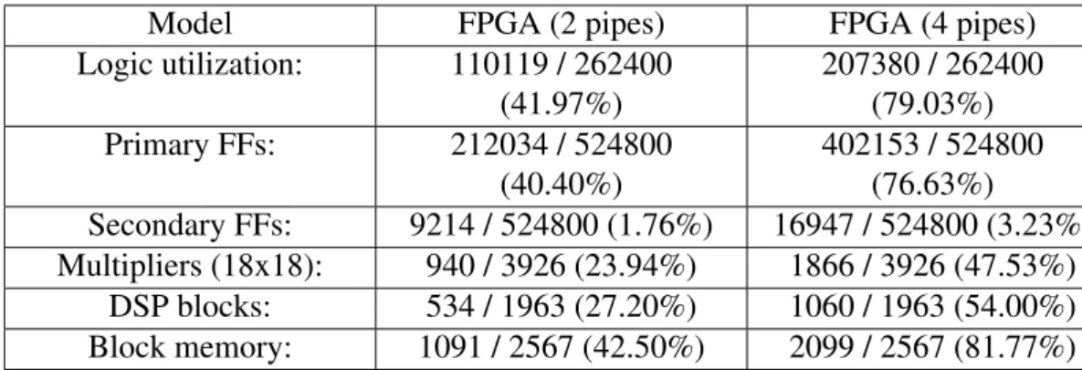
4.1 Resource utilization for the FPGA implementation . . . 64

5.1 Lower and upper bounds for the Heston model calibration . . . 72

5.2 Performance comparison of the sequential implementation for the

He-ston model calculation with the QuantLib Library 1.9. Tests have been performed on an Intel Core i7-4810MQ CPU 2.80GHz with 8GB

RAM memory . . . 75

5.3 η– the achieved speedup vs. the maximum theoretical speedup x 100 %. 76

5.4 MC: percentage_nodes – the computational percentage cost spent on a

sequential code . . . 76

5.5 MC:η– the achieved speedup vs. the maximum theoretical speedup x

100 %. . . 77

5.6 percentage_nodes – the computational percentage cost spent on a

se-quential code . . . 77

5.7 Simulation and calibration times during the calibration process for

10000 paths . . . 80

5.8 Calibration results for 10000 paths . . . 80

5.9 Calibration results for 23 call options with 2 maturities – 10000 paths,

100 timesteps . . . 81

5.10 Calibration results for 10000 paths – SPX 500 call options . . . 82

5.11 Calibration results for 10000 paths – SPX 500 put options . . . 87

5.12 Calibration results for 10000 paths – Dow-Jones Industrial Average

(6)

5.13 Calibration results for 10000 paths – Dow-Jones Industrial Average

index put options . . . 96

5.14 Calibration results for 10000 paths – BP call options . . . 100

5.15 Calibration results for 10000 paths – BP put options . . . 104

5.17 Simulation and calibration times during the calibration process for 10000 paths and 300 timesteps . . . 110

5.18 Calibration results for 10000 paths . . . 110

5.20 The computation times of option prices, sensitivities via the Finite Dif-ference methods and FD. The computational experiments have been performed on an Intel Core i7 -4810MQ 2.80 GHz with 8 GB RAM. . 112

5.21 η– the achieved speedup vs. the maximum theoretical speedup x 100 %.113 5.22 Execution times for the semi-closed form Heston model calibration using the Adjoint on HPC . . . 113

5.23 The sensitivity calculation for the semi-closed form Heston model – DAG size (10653 nodes) . . . 114

5.24 Calibration results for 10000 paths – SPX 500 call options . . . 116

5.25 Calibration results for 10000 paths – Dow-Jones Industrial Average index call options . . . 120

(7)

List of Figures

3.1 Chain-rule of the Black-Scholes model as a DAG . . . 32

4.1 Architecture – Model Definition . . . 50

4.2 DAG processing on HPC platforms . . . 50

4.3 Architecture – High-Performance Engine for Monte-Carlo simulation

and model calibration . . . 56

4.4 HPC Engine for MC simulation – Model Definition . . . 57

4.5 Architecture – High-Performance Engine for Monte-Carlo simulation

and model calibration . . . 58

4.6 HPC Engine for MC simulation – Parameter definition . . . 59

4.7 HPC Engine for MC simulation – Processing flow . . . 59

4.8 Architecture – HPC Engine for Monte-Carlo simulation and model

cal-ibration . . . 60

4.9 Architecture – HPC Engine for Monte-Carlo simulation and model

cal-ibration . . . 61

4.10 DFE graph for the Heston model . . . 63

4.11 Architecture – HPC engine for Non-linear least squares optimization . 66

4.12 Non-linear least-squares optimization framework – Objective Function

Definition . . . 69

4.13 Non-linear least-squares optimization framework – Processing flow . 69

5.1 Performance results – Differentiation vs. Pricing . . . 73

5.2 Performance results – OpenCL NVIDIA K40 vs. OMP (a

single-thread implementation) . . . 78

5.3 Database query for call option price matrix for S&P 500 index . . . . 81

5.4 Implied volatility . . . 84

5.5 Database query for put option price matrix for S&P 500 index . . . . 86

(8)

5.7 Database query for call option price matrix for Dow-Jones Industrial

Average index . . . 91

5.9 Database query for put option price matrix for Dow-Jones Industrial Average index . . . 95

5.11 Database query for call option price matrix for BP . . . 99

5.13 Database query for put option price matrix for BP . . . 103

5.15 Database query for call option price matrix for S&P 500 index . . . . 115

5.16 Database query for call option price matrix for Dow-Jones Industrial Average index . . . 119

(9)

Abstract

C

ALIBRATION OF FINANCIAL MODELS BASED ON

A

UTOMATIC

DIFFERENTIATION AND

HIGH-PERFORMANCE

COMPUTING

Grzegorz Kozikowski

A thesis submitted to the University of Manchester

for the degree of Master of Philosophy, 2018

Stochastic models are commonly used in quantitative finance to describe the dy-namics of the derivatives market. As the market quotes are constantly changing, the models need to be calibrated to make real-time investment decisions. This can involve the sensitivity calculation to support the calibration process and investment portfolio management. For investment portfolios consisting of thousands of assets and options, the sensitivity calculation and calibration process are computationally expensive.

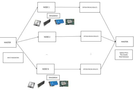
This thesis presents a number of approaches to sensitivity calculation and model calibration utilizing high-performance computing architectures and Automatic Differ-entiation that improve performance and accuracy in financial modeling when com-pared to finite differences and pathwise methods. A parallel Monte-Carlo engine has been developed using the Adjoint methods for the first-order sensitivity calculation and model calibration This addresses the sensitivity and calibration problem for gen-eral stochastic differential models. The engine supports multi-/many-core CPU, GPU and distributed computing architectures. The work utilizes a graph representation and overloading operators to express general stochastic differential models. The sensitiv-ities for the model calibration are calculated in parallel via a single simulation by the

Adjoint method with the gradient computation cost being 1.8xthat of function

evalua-tion. The computational experiments consider both the Heston model and Heston with term-structure. These show that the engine improves performance by up to two orders of magnitude when compared to a sequential version. A hardware implementation has been developed for the Heston model calibration via the Adjoint on FPGA. The work also shows performance improvement of up to two orders of magnitude when com-pared to a sequential implementation. A parallel non-linear least squares optimization framework using Automatic Differentiation has been developed. This utilizes a graph representation and overloaded operator techniques to express the general objective and constraint functions. The framework supports multi-/many-core architectures such as GPUs and Intel Xeon/Xeon-Phi. The computational experiments consider the semi-closed form Heston model with the Gauss-Kronrod integration. These show

perfor-mance improvement of 8.4x on GPU (OpenCL) and 7x on (CUDA) vs a sequential

OMP (OpenMP) implementation. A Xeon-Phi implementation improves performance

(10)

Declaration

No portion of the work referred to in this thesis has been submitted in support of an application for another degree or qualification of this or any other university or other institute of learning.

(11)

Copyright

i. The author of this thesis (including any appendices and/or schedules to this the-sis) owns certain copyright or related rights in it (the “Copyright”) and s/he has given The University of Manchester certain rights to use such Copyright, includ-ing for administrative purposes.

ii. Copies of this thesis, either in full or in extracts and whether in hard or electronic

copy, may be madeonlyin accordance with the Copyright, Designs and Patents

Act 1988 (as amended) and regulations issued under it or, where appropriate, in accordance with licensing agreements which the University has from time to time. This page must form part of any such copies made.

iii. The ownership of certain Copyright, patents, designs, trade marks and other in-tellectual property (the “Inin-tellectual Property”) and any reproductions of copy-right works in the thesis, for example graphs and tables (“Reproductions”), which may be described in this thesis, may not be owned by the author and may be owned by third parties. Such Intellectual Property and Reproductions cannot and must not be made available for use without the prior written permission of the owner(s) of the relevant Intellectual Property and/or Reproductions.

iv. Further information on the conditions under which disclosure, publication and commercialisation of this thesis, the Copyright and any Intellectual Property and/or Reproductions described in it may take place is available in the

Univer-sity IP Policy (seehttp://documents.manchester.ac.uk/DocuInfo.aspx?

DocID=487), in any relevant Thesis restriction declarations deposited in the

Uni-versity Library, The UniUni-versity Library’s regulations (seehttp://www.manchester.

ac.uk/library/aboutus/regulations) and in The University’s policy on pre-sentation of Theses

(12)

Glossary

The following table presents an explanation of financial terms mentioned in this work [Hul12]

(13)

Name Description

American Option An option that can be exercised at any time during its life

Arbitrage A trading strategy that takes advantage of two or more securities being

mis-priced relative to each other

Ask Price The price that a dealer is offering to sell an asset

Barrier Option An option whose payoff depends on whether the path of the underlying asset

has reached a barrier (i.e. a certain predetermined level)

Bid Price The price that a dealer is prepared to pay for an asset

Bid-Ask Spread The amount by which the ask price exceeds the bid price

Calibration Method for implying a model’s parameters from the prices of actively traded

assets

Call Option An option to buy an asset at a certain price by a certain date

Derivative An instrument whose price depends on, or is derived from the price of

an-other asset

Discount Rate The annualized dollar return on a Treasury bill or similar instrument

ex-pressed as a percentage of the final face value Euler-Maruyama

method

A method for the approximate numerical solution of a stochastic differential equation

European option An option that can be exercised only at the end of its life

Exercise (Strike)

Price

The price at which the underlying asset may be bought or sold in an option contract

Expiration date The end of life of a contract

Feller condition the condition for which the volatility of the Heston model is strictly positive

Implied volatility Volatility implied from an option price using the Black-Scholes formula

Interest Rate Interest Rate defines the amount of money which is paid to a borrower by

the lender and is a key factor in pricing interest rate derivatives (contracts whose value depends on the interest rate fluctuations)

Kantorovich Graph (DAG)

a graph representing chain-rule of the function subsequent operations nec-essary to evaluate the value of a function

Maturity the end of the life of a contract

Newton-Raphson Method

An iterative procedure for solving nonlinear equations

Option a contract that gives the right to buy or sell an asset

Payoff The cash realized by the holder of an option or other derivative at the end of

its life

Put Option An option to sell an asset for a certain price by a certain date

RMSE Root Mean Square Error

Strike price the price at which the asset may be bought or sold in an option contract (also

called the exercise price)

Volatility A measure of the uncertainty of the return realized on an asset

Volatility Skew A term used to describe the volatility smile when it is nonsymmetrical

Volatility Smile The variation of implied volatility with strike price

Volatility Surface A table showing the variation of implied volatilities with strike price and

time to maturity

Wiener Process A process where the change in a variable during each short period of time of

length t has a normal distribution with a mean equal to zero and a variance equal to t

(14)

List of abbreviations

The following table presents a list of abbreviations used in this thesis.

Name Description

AD Automatic Differentiation

CPU Computational Processing Unit

DAG Directed Acyclic Graph

FFT Fast Fourier Transform

FPGA Field Programming Gateway Array

GPU Graphics Processing Unit

HPC High-Performance Computing

MC Monte-Carlo simulation

OpenCL Open Computing Language

OpenMP Open Multi-Processing

PDE Partial Differential Equation

RMSE Root Mean Square Error

SDE Stochastic Differential Equation

(15)

Chapter 1 Introduction

This thesis presents approaches to financial derivatives pricing, the Greeks’ calcula-tion and model calibracalcula-tion using numerical methods such as Automatic Differentia-tion, Monte-Carlo (MC) methods and High-Performance computing (HPC) platforms such as FPGA cards, GPUs, multi-core and many-core processors. The presented approaches utilize overloading operator techniques and graph processing to support general stochastic models. This combination improves performance and accuracy of financial option pricing, the Greeks’ calculation and model calibration by up to two orders of magnitude. The work can find application in real-time risk management systems and derivatives trading platforms.

Over the last 30 years derivatives – financial instruments whose value depends on underlying assets such as stocks, stock indices, interest rates, foreign exchange rates and commodities such as oil, gold, silver – have become increasingly important in finance. The amount of outstanding derivatives positions was close to $500 trillion by January 2016 [otc16]. These contracts are traded on the over-the-counter markets. The fundamental derivatives contract is an option which gives the client the right to buy or sell the given commodity at a certain time with the price negotiated at the present time. The negotiated price is called the exercise or strike price. The date of the contract is known as the expiration date or maturity. There are two types of options: call, which gives the investor an opportunity to buy the asset, and put, which is to sell the traded instrument. Further, the call and put options can be sold and purchased.

In addition, there are varieties of options such as American, European, Asian and barrier options. American options can be exercised at any time until expiration date; European options can be exercised at the expiration date only; The Asian options de-pend on the average price of the underlying asset over a certain period of time; the

(16)

barrier options depend on whether the underlying asset has exceed the predetermined price. When buying a call or put option, a buyer is referred to as having a long position. When selling a call or put option, a seller is referred to as having a short position. The derivatives market uses option price makers to ensure market liquidity. Option market makers quote a bid and ask price – the bid price is the price at which the option mar-ket maker is prepared to buy an option, the ask price is the price at which, the marmar-ket maker is prepared to sell [Hul12].

There are several factors affecting an option price such as: the current stock price, the strike price, the time to expiration, the volatility of the stock price, the risk-free interest rate and the dividends. The volatility of the stock price measures a degree of changes of the stock price over time. Over the last three decades, several models have been derived to describe the dynamics of options on various underlying assets such as European options, interest rate options, etc. The simplest approach, binomial tree, based on constructing a binomial tree was introduced by Cox, Ross and Rubinstein in 1979 [CRR79]. The binomial tree, also known as the lattice model, describes an evo-lution of the option price in discrete time. This consists of the nodes representing the stock price and option price. In 1973, Black, Merton and Scholes derived the model for option pricing based on stochastic calculus [BS73]. The model assumes that the

stock price follows a geometric Brownian motion with the driftµand the variance rate

σ– the process with log-normal distribution. The European option price is calculated

as the discounted value of the difference between the strike price and the stock price at expiration date. This model assumes that the volatility of the commodity is con-stant over time. In risk management, implied volatility is calculated – the volatility for which the Black-Scholes formula produces the market option price. As the volatility of commodities is non-constant over-time, the Heston model was introduced, which assumes that volatility follows a stochastic mean-reverting process [Hes93]. Further, many derivations were introduced using the Jumps Poisson process to express com-modity price jumps caused by various events [Gat06]. There are several methods for solving the Heston model such as Monte-Carlo simulation, finite difference methods and the maximum likelihood method. Monte-Carlo simulation involves random num-bers to produce many different paths of the option price. The arithmetic average of the payoffs is the estimated value of the option price. Finite-difference methods solve the Partial Differential Equations (PDE) by using the difference equation [Gla04]. The maximum likelihood method maximizes the likelihood function [MPZ08a]. Further, the European option price for the Heston model can be derived analytically by using

(17)

the characteristic function of the option price distribution. This involves integration of a complex formula and can utilize the FFT methods, or quadrature-integration meth-ods.

One of the investment strategies using options is hedging, which allows financial institutions to neutralize risks of market movements by contracting commodity price. Hedging often involves application of mathematical modelling to the derivatives mar-ket to measure financial risks. The mathematical modelling in the derivatives marmar-ket can be used to price options for different maturities and strikes and to calculate the Greeks – risk sensitivities that measure how the model parameters affect the option price. Financial institutions use the Greeks to manage and hedge investment portfo-lios (to compensate loss on the market by gains made on another market and stabilize portfolio value).

As an example, consider an investor wishing to neutralize his portfolio from further commodity price movements by delta-hedging [Hul12]. For this purpose, he calculates the Greek that measures how the change of the underlying asset price affects the op-tion price (delta). Based on this value, he constantly adjusts his investment posiop-tions to cover further gains (or loss) on the stock market by loss (or gains) on derivatives market/options. This means that his overall portfolio value will remain constant for a short time (as option prices and stock prices permanently fluctuate). To mitigate risk of movements on his portfolio, he must constantly re-calculate the Greeks and rebalance the positions. For portfolios consisting of thousands of underlying assets and options traded by banks every day, frequent rebalancing based on the Greeks (via Monte-Carlo simulation) is computationally demanding.

Further, option pricing and the Greeks’ calculation for a given asset on the market require the model calibration to the historical market-data. There is need to determine such a set of model parameters for which the model accurately expresses past market-quotes. The option model calibration is analytically expensive as this often requires the gradient calculation the first-order Greeks – the first-order derivatives of the option payoff with respect to the input parameters) – to fit hundreds of market quotes and thousands of different underlying assets every day [Hul12]. Most existing solutions for the Greeks’ calculation are based on the pathwise, likelihood or finite differences methods, in which computational cost of the gradient is at least proportional to the

(18)

1.1 Aims and Objectives

This thesis aims at:

• performance and accuracy improvement in model computation, sensitivity

eval-uation and model calibration in financial applications by utilizing high-performance computing platforms and numerical methods such as Automatic Differentiation;

• flexible definition of various models and discretization schemes used in

deriva-tives pricing and hedging. This aims at utilization of overloading operator tech-niques and graph processing

The work focuses on the Heston model calibration (the Heston with the Feller con-dition, the Heston model with Jumps, the Heston model with term-structures and the semi-closed form Heston model solution).

1.2 Contribution

The contribution of this work is performance and accuracy improvement in financial model calibration and sensitivity calculation. For this purpose, several calibration frameworks have been implemented that combine numerical methods as Automatic Differentiation and HPC platforms. The calibration frameworks have been tested with a financial case-study: Heston-model calibration.

The detailed aspects of the contribution include:

• A parallel MC engine for the first-order sensitivity calculation and model

cali-bration using the Adjoint.

This work utilizes a graph representation and overloading operators to express general stochastic models. The sensitivities for the model calibration are cal-culated in parallel via a single simulation by the Adjoint method with the

gra-dient computation cost being 1.8x that of function evaluation. The framework

supports multi-, many-core and distributed architectures such as GPUs, Intel-Xeon/Xeon-Phi with the frameworks CUDA, OpenCL, OpenMP with Xeon-Phi and OpenMPI.

The engine provides an interface that allows a platform-independent model def-inition. The computational experiments consider the Heston model and Heston with term-structure. These show that the engine improves performance by up to

(19)

two orders of magnitude when compared to a sequential version. This is pro-vided as a static and dynamic library.

• Heston model calibration using the Adjoint and MC methods on FPGA - a MC

engine for the expected value computation, the first-order Greeks calculation and model calibration. The sensitivities are calculated in parallel via a single simulation by the Adjoint - an Automatic Differentiation method with the

gra-dient computation cost being 1.8 xthat of function evaluation. The gradient is

applied to the optimization methods to calibrate the model to market data. The framework supports FPGA cards with Maxeler technology. The computational experiments consider a financial case-study: the Heston model calibration.

• Parallel non-linear least squares optimization framework using Automatic

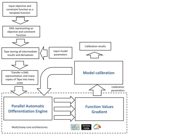
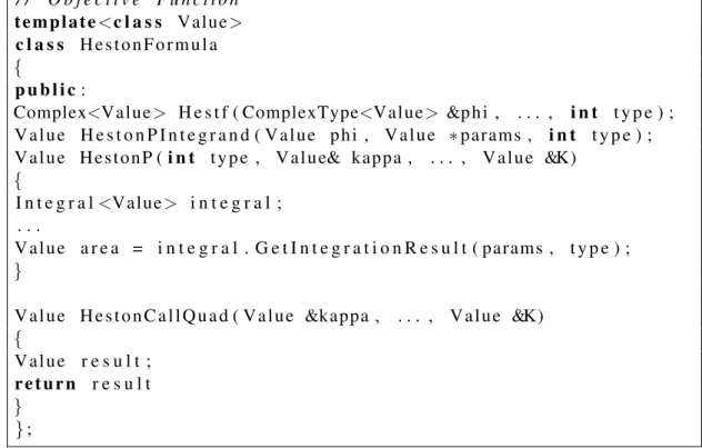
Dif-ferentiation – this work presents a parallel non-linear least squares optimization framework using Automatic Differentiation. This approach utilizes a graph rep-resentation and overloaded operator techniques to express the general objective and constraint functions. The framework computes values and the gradient of the objective/constraint function at many different points in parallel. The gra-dient for the non-linear least squares optimization is calculated in parallel with the computational cost being twice that of function evaluation. The gradient is applied to the non-linear least squares optimization methods. The framework supports multi-, many-core architectures such as GPUs, Intel Xeon/Xeon-Phi with the frameworks CUDA, OpenCL, OpenMP with Xeon-Phi. The computa-tional experiments consider the semi-closed form Heston model with the Gauss-Kronrod integration method.

1.3 Structure

The rest of this thesis is structured as follows: Chapter 2 presents a review of related literature; Chapter 3 presents the technical context of the work; Chapter 4 presents parallel frameworks for financial sensitivity calculation and model calibration; Chap-ter 5 presents computational experiments for the Heston model calibration on High-Performance Computing platforms; Chapter 6 presents conclusions and further work.

(20)

Chapter 2 Literature review

2.1 Introduction

This section provides a literature review concerning Automatic Differentiation, Monte-Carlo (MC) methods, model calibration and high-performance computing (HPC) in the context of scientific and industrial applications. This is divided into three sections corresponding to the contribution areas:

1. Section 2.2 reviews work on Automatic Differentiation (AD), MC simulation and HPC applied to scientific and industrial applications;

2. Section 2.3 reviews research on financial simulation and model calibration using FPGA cards;

3. Section 2.4 reviews advances on AD tools and their application in optimization.

2.2 Parallel Monte-Carlo (MC) engine for the first-order

sensitivity calculation and model calibration using

the Adjoint

Monte Carlo (MC) simulation is a procedure for sampling random scenarios for the input process and evaluating the expected value converging to the correct result. This method is widely used to solve stochastic models for which the analytical solutions are

(21)

too complex to derive. This is used in finance for pricing and hedging complex deriva-tives contracts. Unfortunately, MC simulation is computationally expensive when cal-culating the output result, with the computational cost increasing with the number of scenarios. Furthermore, the sensitivity and model calibration is computationally demanding. The calibration can utilize the gradient information to support local opti-mization methods.

Several differentiation methods can be used with MC simulation to evaluate the first-order sensitivities to support model calibration. The simplest, the finite difference (FD) method, requires two MC simulations that differ in a small change in a single

input model parameter [FHP+12]. Based on these MC results, the sensitivity is

calcu-lated as the ratio of the output change to the small change in the input parameter. Un-fortunately, this method is both computationally expensive (the first-order sensitivities

require (2xmodel parameters)xthe cost of a single MC simulation) and inaccurate if

the change is too big. The likelihood method utilizes the probability density functions, therefore, they can be applied to non-smooth models but often produce inaccurate re-sults with large variance. Pathwise methods are based on AD with the forward order. They require as many MC simulations as the number of model parameters to evaluate the sensitivities. The pathwise method for the sensitivities has a computational cost generally smaller than finite differences. The drawback of this technique is complexity

in the case of models with a large number of independent variables [FHP+12].

Work in [Zha13] presents a HPC engine for the Value at Risk (VaR)

computa-tion using the MapReduce model. The Map funccomputa-tion splits the dataset into small data chunks and distributes these to processing nodes. The Reduce function collects the results from the nodes and generates the output result. This paradigm is used to paral-lelize MC simulation for the VaR. Performance experiments have been performed on a cluster of 4 nodes. The execution time of the sequential MC simulation was around 532 seconds;the parallel MC simulation computes VaR in around 115 seconds.

Work in [Mih15] presents approximations to option sensitivities for stochastic volatil-ity models. These utilize a sequential MC techniques for the latent state in a Hidden Markov Model. These techniques are applied to the Greeks’ computation using the likelihood ratio method. Further, the work develops a modified explicit Euler scheme for SDEs with non-Lipschitz continuous drift or diffusion.

Work in [Mor06] presents a parallel option pricing framework for interest rate derivatives via the Hull-White trinomial interest rate lattice model. This applies vec-torization and data parallelization techniques available in Fortran. The parallel pricing

(22)

includes the classical backward induction and MC simulation. The implementation supports distributed computing with shared memory.

Work in [Ras16] presents an approach to the Dupire’s deterministic local volatil-ity function calibration. The work compares performance for five different calibration methods for the local volatility function. Further, the work presents approaches to eval-uating the first-order derivatives: complex-step derivative approximation, automatic differentiation forward mode and reverse mode. These are utilized to calculate the

Greeks forCredit Value Adjustment(CVA) for an interest rate swap. The work utilizes

FADBAD++ – an AD tool for the derivatives calculation. The work does not support the derivatives calculation on parallel and distributed architectures.

Work in [Doa10] presents a HPC engine for MC simulations for financial ing applications. This introduces a grid programming framework for derivatives pric-ing. The framework supports fault-tolerance, load balancing, dynamic task distribution and deployment mechanism for heterogeneous grid architectures. Further, the work presents an implementation of a Classification MC algorithm for high-dimensional American option pricing. This is scaled up to 64 processors in a grid environment.

Work in [PSLvL16] presents application of the automatic differentiation forward mode to solving mass transfer equations. This applies the Newton method for solv-ing non-linear equations. AD was combined with block and band compression for efficiently computing the Jacobian. For the derivatives computation, ADOL-C was utilized. The work compares the forward AD mode with FD method and analytical derivations for the first-order derivatives. The approach using the analytical deriva-tions for the Jacobian was two times faster than the forward AD mode. The work does not utilize the Adjoint method. This does not support parallel processing on HPC platforms.

Work in [DZ13] presents an implementation for stochastic volatility model calibra-tion on a multi-core CPU cluster. The implementacalibra-tion utilizes shared and distributed packages in Python. The computational experiments consider the Heston and Bates models. The experiments have been performed on a cluster of 32 dual socket Dell

PowerEdge R410 nodes providing 256 cores. The speed-up achieved is around 139x

against the sequential version. This reduces overall time taken to calibrate 1024 SPX

options by a factor of 37x.

Work in [Cap11] gives an approach to calculating sensitivities of stochastic differ-ential processes. The underlying idea is an application of the Adjoint to each scenario

(23)

of the MC simulation for solving stochastic differential equations (SDE). The compu-tational cost of the sensitivity calculation via the Adjoint is independent of the number of input parameters of the stochastic model. Derivatives are calculated by utilizing the Adjoint in the rules required to calculate the final result (chain-rule). Considering a system depending on 60 parameters and providing the SDE solution in 1 minute, this typically computes the gradient in less than 4 minutes. Unfortunately, this work does not exploit parallel architecture.

Work in [GHR+16] presents an approach to the gradient calculation using the

Ad-joint techniques on GPU architectures. This utilizes vector and matrix structures to store intermediate partial derivatives. The work studies performance for four cost func-tions: sum of sigmoids, linear leasts-squares, maximum entropy models and Cholesky decomposition. The computational experiments have been performed on an Intel Xeon e-5-1620 v2 (3.7 GHz) with 64 GB of DDR3 RAM memory and an NVIDIA GeForce

GTX Titan Black. The speedup achieved on GPU cards is around 7.5x±4.4 vs. a

se-quential implementation on CPU. In this implementation, the multiple threads located on GPU cannot create their own tapes.

Work in [SZAW15] presents parallel approaches to option pricing utilizing the lattice model and the MC method. The work has been implemented in CUDA and OpenCL. This utilizes the Black-Scholes model for option pricing. Benchmarks have been performed for the option pricing via the Black-Scholes model. Computational experiments have been done on an Intel Dual Core Xeon processor with 3.4GHz with 16GB RAM memory and NVIDIA GeForce GTX 980 with 4GB RAM memory. Pric-ing of an option with 100000 timesteps on a CPU via the lattice method requires around 23K ms whereas a parallel version computes option prices in around 3.5K ms. The MC simulation for 1000000 paths and 1000 timesteps takes around 186 seconds on a CPU. The parallel GPU version of the MC simulation calculates the option prices in around 6 seconds for 1000000 scenarios and 100 timesteps on GPU. The work does not allow the sensitivity computation and does not support general stochastic models.

Work in [MF12] applies AD to the quadrature – numerical integration to calculate the sensitivities of the integral. There are included derivations for truncation errors. The results hold when the integrand is one degree higher continuously differentiable than the sufficient for convergence of its quadrature. The work is tested with a tetra-choric correlation estimation example in Matlab. This utilizes rectangle, midpoint and Simpson’s rule for integration. The work uses forward mode automatic differentiation for the derivatives calculation. The work does not support automatic differentiation in

(24)

reverse mode.

Work in [JY11a] considers application of the Adjoint to MC simulation for the gamma matrix computation for multidimensional financial derivatives including Asian

baskets and cancelable swaps. Numerical results show that computation of all n(n+

1)/2 gammas in the LMM takes approximatelyn/3 times as long as computing the

price.

Work in [JY11b] presents the application of the Adjoint techniques to the Delta computation of interest rate derivatives. The work studies constant maturity swap rate market model and co-initial swap-rate market model. The work shows that the

com-putational complexity of the algorithm is proportional to the number of rates x the

number of factors per step.

Work in [CL14] presents an application of automatic differentiation and the Im-plicit Function Theorem to sensitivity calculation and model calibration for the credit default swaps and credit default index swaptions. The computational experiments for

the credit default swaps shows performance improvement by up to 50xfor 18 spread

tenors and interest rate instruments. The combination of automatic differentiation and the Implicit Function Theorem allows computation of interest rate and credit spread risk in 20 % less time than computation cost of option price. The work does not sup-port processing on parallel architectures.

Work in [LL14] addresses an implementation for pricing Asian Options on an Intel Xeon-Phi Coprocessor architecture. This utilizes a closed-form analytical solution for the geometric average Asian option and MC method for the arithmetic average Asian option. The work was compared with a single-Asian option example included in CUDA SDK 6.0 on an NVIDIA Tesla K40c. Experimentation shows that the pricing of a 2-year contract with 252 time steps and 1M scenarios takes around one fifth of a second on an Intel Xeon-Phi Coprocessor 7210p. The GPU implementation calculates the Asian option price in around 0.469 second. The work does not support graph processing to define general stochastic models on a multi-core Xeon-Phi architecture. Further, this does not support the sensitivity calculation.

Work in [FBI06] applies the Adjoint in seismology. The changes to displacement field and flow patterns at the surface can be quantified with respect to the changes of density, viscosity or elastic coefficients. The work derives the equations for the scalar wave dynamics in two dimensions. A numerical case-study shows that the Adjoint focuses near to the location of a parameter perturbation at the same rate when the original wavefront reaches that location and the Adjoint is far more efficient than finite

(25)

difference approximations. This does not rely on the existence of Green’s functions or transposes of a differential operator. To locate parameter perturbations, the least-square function with the Adjoint is utilized. The method can be applied to non-linear operators using the Navier-Stokes equations. Work [DLS10] presents an implementation of the Adjoint MC method in Geant4 – a toolkit for simulation of the passage of particles through matter and the GRAS module (Geant4 Radiation Analysis for Space). This aims at precise computation of space radiation effects on electronic components, solar panels and optical devices in complex payload and satellite geometry. It compares the Pathwise forward and the Adjoint methods to analyze two test geometries presenting the components. The numerical results show that the Adjoint improves performance by up to four orders of magnitude when considering the sensitive volume size equal to 1 mm.

The Adjoint with MC simulation of the European option was applied to the He-ston calibration in [KMS09]. For the optimization process, the standard sequential quadratic programming methods with the Gauss-Newton approximation of the Hessian were utilized. Tests were performed on a 3 GHz CPU and 2 GB memory. As expected, the algorithm reduced the number of MC simulations for different partial derivatives (usually evaluated by FD approximations). The presented approach improves the cali-bration time for a typical equity market model with time-dependent model parameters calibrated by the FD method from over three hours (approx 200 minutes) to less than ten minutes. Unfortunately the sequential solution is strongly dependent on the starting points as the problem is non-convex, thus it converges to the nearest local minimum. The accuracy experiments showed that the Adjoint implementation produces the same result as the FD approach. The implementation was only executed on a single CPU core, hence, it may be worth investigating parallel computing for the MC-based cali-bration.

Calibration of the Heston stochastic volatility model using filtering and maximum likelihood methods is presented in [MPZ08b]. A standard steepest ascent method for a non-convex maximum likelihood function was utilized to optimize the maximum like-lihood function. As evaluation of the maximum likelike-lihood function is computationally demanding, parallel architectures were used to boost performance. The implementa-tion was tested on a IBM SP4 machine with 32 processors. The speedup factor was equal to 15x for 16 processors used. The accuracy of the calibration of European

options was about 10−5(the value of the Root Mean Square Error (RMSE) function).

(26)

to evaluation of the first-order Greeks using the standard MC simulation. This uti-lizes parallel GPU architectures such as NVIDIA CUDA to boost performance. The first-order Greeks are calculated through the MC simulation for Black-Scholes and the Heston model. This uses derivations for specific financial models and cannot be ap-plied to general SDE models. The parallel experiments are compared with a sequential implementation and run on an NVIDIA Tesla C2070 with 448 cores. They show an improvement of approximately two orders of magnitude for both the Black-Scholes and the Heston first-order Greeks.

2.3 Heston model calibration using the Adjoint and MC

methods on FPGA

Work [dSSK+11] presents a hardware implementation of an MC simulation for the

Heston model for European options. The approach developed in VisualHDL on a Xilinx Virtex-5 doubles performance compared with a CPU equipped with an Intel Xeon CPU W335 3.07 Ghz and 8 GB RAM. Unfortunately, the implementation does not support the Greeks calculation and model calibration.

Work [SRMLB+13] explores an FPGA implementation of an MC method to price

Asian options via the Black-Scholes model on an FPGA Altera Stratix-V card. The approach has been developed in the Impulse C environment supporting floating-point arithmetic on the FPGA. For generating normal distribution random samples, the Mersenne Twister with Box-Muller transform has been utilized. The results show performance

improvement of the FPGA implementation by 504xwhen compared to an execution on

a single-core implementation (Intel i7 850 2.8 Ghz) and approx. 150xwhen compared

with a 4-core implementation supported by OpenMP. The implementation only inves-tigates the Black-Scholes model which does not allow risk sensitivities calculation and model calibration.

Work [TB08] explores an FPGA engine for solving the Black-Scholes model via MC simulation. This is benchmarked on a Maxwell Supercomputer equipped with 64 FPGA Xilinx Virtex-4 XC4VSX55 cards and compared against a 32 core CPU cluster.

The speed-up achieved was around 750xcompared to the CPU cluster. This work only

presents the Black-Scholes model and does not evaluate the Greeks.

Work of [JLT11] addresses a FPGA framework to solve option pricing formulas via different methodologies: MC, FD, quadrature method and binomial trees. As case

(27)

studies both European and American options are considered. The MC simulation

Eu-ropean options on an FPGA is 41x faster compared with an 8 core Intel Xeon CPU

processor. This work does not allow risk sensitivity calculation and model calibration. Studies presented in [NAW08] explore a Quasi MC method for option pricing

us-ing Brownian paths. The performance results in a 50xspeed-up on an FPGA (Altera

Stratix III EP3SE260-3) compared with an Intel Xeon 3 GHz CPU. This work does not support more complicated option pricing models, such as the Greeks’ calculation and calibration to market data.

2.4 Parallel non-linear least-squares optimization

frame-work using Automatic Differentiation

There are several tools that support the gradient calculation via AD. These generally present two approaches for the recording chain-rule: source-code transformation or operator overloading.

Work in [WG10] presents an open-source package in C/C++ for AD. The work supports overloading operator techniques to define differentiable functions. This al-lows the first and higher-order derivatives calculation in forward and reverse automatic differentiation mode. This supports MPI and OMP parallel programs. Unfortunately, this does not support many-core and GPU architectures.

Work in [HP13] presents an AD tool that supports the adjoint derivatives and tan-gent calculation. The software allows differentiation of function written in C++ and Fortran. The software does not support differentiation on parallel architectures.

Work in [Hog14] presents an approach to the first-order derivatives calculation in reverse-mode AD. The work utilizes Expression C++ templates. The work utilizes overloaded operator techniques to build a graph representation of a model function. The work has been incorporated into the Adept library. Benchmarks for four differ-ent numerical algorithms show the performance improvemdiffer-ent against other operator-overloading libraries. ADOL-C is 5-7 times slower than Adept, CppAD is 7-9 times more expensive and Sacador is 2.6-8 times slower than Adept. The work reduces memory usage being 1.3-7.7 times more efficient. The work does not support complex arithmetic and differentiation on parallel computing architectures.

Work in [FSA+12] presents an AD framework for solving statistical parameter

(28)

a large number of parameters. The software provides functionality of analysis of un-certainty of estimated parameters via a Markov-chain MC method. The framework utilizes overloading operator techniques to record chain-rule of the model function. The software transforms the source-code with the model definition into C++. Next, the C++ code is compiled and linked with the AD library to create a binary program. Unfortunately, the software does not support differentiation on HPC architectures.

Work in [GHR+16] presents an approach to the gradient calculation utilizing the

Adjoint methods on GPU architectures. this uses vector and matrix data structures to store intermediate partial derivatives The work studies performance for four cost func-tions: sum of sigmoids, linear least-squares, maximum entropy models and Cholesky decomposition. The computational experiments have been performed on an Intel Xeon e-5-1620 v2 (3.7 GHz) with 64 GB of DDR3 RAM memory and an NVIDIA GeForce

GTX Titan Black. The performance improvement on GPU is around 7.5x±4.4 vs.

a sequential implementation on CPU. In this implementation, the multiple-threads lo-cated on GPU cannot create their own tapes – data structures to store intermediate results and the first-order sensitivities.

Work [ABFK11] proposes an approach to the Heston model calibration using global optimization methods. The Heston model is evaluated by using the Fourier cosine method on CUDA. The model has been evaluated for many sample points distributed with quasi-distribution over the parameter space. Further, the Levenberg-Marquardt method has been applied to the most feasible points (the points for which RMSE is low). The gradient for optimization was evaluated using the FD method. Performance studies have been done on a GPU server with two NVIDIA GPU C1060 and one GTX 260. The implementation was benchmarked with a varied number of generated random samples (from 256 to 65536). The experiments have been carried out for one option set (256 options). Performance improvement has been achieved for 65536 samples;

execu-tion times on a GPU were 50xtimes faster than on a CPU. The optimization algorithm

does not utilize differentiation techniques as the Adjoint to improve performance. Previous work by the thesis author [KK13] presents an application of the Adjoint techniques to the first-order sensitivity calculation via the standard MC simulation. This utilizes parallel GPU architectures to improve performance. The first-order sensi-tivities are calculated through the MC simulation for Black-Scholes and Heston model. This uses derivations for specific financial models and cannot be applied to general SDE functions. The parallel experiments are compared with a sequential implemen-tation and run on an NVIDIA Tesla C2070 with 448 cores. They show performance

(29)

improvement of approximately two orders of magnitude for both the Black-Scholes and the Heston first-order sensitivity computation.

Previous work by the thesis author in [KK12] presents a parallel approach to eval-uating the gradient and Hessian with both forward and reverse AD modes. The library implemented in C++ uses a generic programming paradigm to dynamically parametrize the data-type. Overloaded operator techniques are used to build a graph representation for factorable functions. The graph representation is transferred to GPU and further processed in parallel. Each thread block evaluates and differentiates a single function. The performance experiments were carried out on an Athlon 2.8 GHz processor with

an NVIDIA GF 9800 GT supporting Tesla architecture. The speed-up is equal to 180x

for functions consisting of 64 nodes (the gradient calculation). The execution times

for the Hessian calculation were 280xfaster on a GPU. The implementation supports

interval arithmetic.

2.5 Summary

In this chapter, the literature review has been presented. The section 2.2 focused on ap-plication of Monte-Carlo simulation, Automatic Differentiation and High-Performance Computing platforms to various scientific and industrial applications. This showed the Adjoint technique reduces the cost of the sensitivity calculation when compared to pathwise forward and finite difference methods. The computational cost of the gradi-ent calculation via the Adjoint is independgradi-ent of the number of input parameters for the stochastic models. The input model for various applications can be represented as a sequence of elementary arithmetic operations. This can utilize overloading operator techniques and graph processing to allow the differentiation via AD.

The section 2.4 investigated automatic differentiation frameworks and the semi-closed form Heston model calibration. The automatic differentiation tools can utilize two approaches for the chain-rule recording: source-code transformation and

over-loading operator techniques. The work [GHR+16] presented a GPU approach to the

gradient computation. This showed the performance improvement by the factor of

7.5x±4.4 vs. a sequential implementation. The work [ABFK11] showed that the

GPU cards improve performance of the semi-closed form Heston model calibration

(30)

Chapter 3 Technical context

3.1 Introduction

This chapter provides overview of technical aspects of this work to contextualise the developments and contributions of the thesis. This is organized as follows:

• Section 3.2 introduces a directed acyclic graph - graph representation that can be

used to express a composite function

• Section 3.3 presents fundamentals of automatic differentiation for the gradient

computation using Forward and Reverse (the Adjoint) modes.

• Section 3.4 presents fundamentals of non-linear least squares optimization.

• Section 3.5 concerns Monte-Carlo simulation

• Section 3.6 briefly introduces high-performance computing platforms

• Section 3.7 presents financial models: Heston model, Heston model with Jumps,

Heston model with term-structure used as case-studies.

3.2 Directed Acyclic Graph

A Directed Acyclic Graph (DAG) is a data structure formed by a collection of nodes and directed edges without a directed cycle. Each node is connected to another, such that there is no way to start at a node v, follow any sequence and end at the same node. Each task can operate on a vector of input data, process the intermediate results and

(31)

return the output data vector. The DAG structure can represent a topology of arithmetic operations required to evaluate a function.

3.3 Automatic Differentiation

Background

Automatic Differentiation (AD) is a set of algorithmic routines to accurately and effi-ciently compute derivatives of a composite function [KK12]. This approach allows the

derivatives computation with machine accuracy1[FHP+12].

AD exploits the fact that each composite function can be interpreted as a sequence (chain-rule) of the elementary operators (as addition, multiplication or exponential, etc.) required for its evaluation. To explain AD, the Black-Scholes formula is used as

an example [FHP+12].

Example Consider the Black-Scholes model and its recursive dependency of

com-modity price from timetto timet+1.

S_t₊₁=S_t·(1+r·dt+σ· √

dt·Z) (3.1)

Suppose, we want to evaluate the Black-Scholes single path from timet tot+1. For

this purpose, we derive a sequence (see Table 3.1a) (chain-rule) of elementary

opera-tions needed to evaluate the underlying asset price at timet+1.

f₁=r·dt f2=1+f1

f3=

√

dt f4=σ· f3

f₅= f₄·Z f₆= f2+f5

f7=St·f6

(a) Chain-rule of the Black-Scholes model

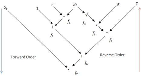
This sequence can be expressed graphically using a DAG (see Figure 3.1) [FHP+12].

The edges represent a dependency between subsequent elementary operators or input

1_{Computational devices use binary systems to represent floating-point arithmetic. The floating-point}

number is represented by using three numbers: sign, exponent and mantissa. Due to the finite number of bits for exponent and mantissa representation, the numbers are rounded to the nearest, toward zero, toward plus/minus infinity [IEE08]

(32)

Figure 3.1: Chain-rule of the Black-Scholes model as a DAG

parameters; the nodes are identified by fi – intermediate functions to evaluate the

fi-nal result. As can be seen, each fi is dependent on some previously computed fj or

model parameters (i> j). It is worth noting that Black-Scholes requires 7

elemen-tary operations to evaluate the underlying asset price at time t+1 from time t with

the forward order. Intuitively, in order to calculate the composite function, we start

computations from independent variables (S_t,..., Z) through intermediate operations

(f₁,...,f₆) to the final operator (f₇). By interpreting such a chain-rule with

forward-order (or reverse) and applying basic differentiation routines for elementary operators, AD computes derivatives of the composite function. These derivatives are accurately evaluated and subject only to rounding and not discretization error. This makes AD particularly attractive when compared to standard numerical differentiation methods, such as finite-differences [Cap11]. AD has two basic modes: Forward (Pathwise) and

Reverse (the Adjoint) [FHP+12].

Pathwise methods

The pathwise method computes derivatives with the forward order and calls differen-tiation routines for elementary functions.

Example Let us perform differentiation of the function from f1to f7 (with the

for-ward order).

First, the derivatives d f₁ and d f₃ are equal to zero as f₁ and f₃ are independent

(33)

f₁=r·dt d f₁=0

f₂=1+f₁ d f₂=d f₁

f₃=√dt d f₃=0

f4=σ·f3 d f4=

dσ·f3+σ·d f3

f₅= f₄·Z d f₅=d f₄·Z f₆= f2+f5 d f6=d f2+d f5

f₇=S_t· f₆ d f₇=S_t·d f₆ (a) Chain-rule of Black-Scholes (Pathwise meth-ods)

f₁=r·dt f₇= d f7

d f7 =1

f2=1+f1 f6= d f_{d f}7₆ ·f7=

St·f7

f₃=√dt S_t= d f7

dSt ·f7=

f₆·f₇ f4=σ·f3 f2= _{d f}d f6₂·f6= f6

f₅= f₄·Z f₅= d f6

d f5·f6= f6

f₆= f2+f5 f4= d f_{d f}5₄ ·f5=

Z·f₅ f₇=S_t·f₆ Z= d f5

dZ · f5= f5

f₃= d f4

d f3 ·f4=

σ·f4

σ=d f_d4 σ ·f4=

f₃·f₄ dt= d f3

ddt ·f3=

1 2√dt·f3

f₁= d f2

d f1·f2= f2

dt+ = d f1

ddt ·f1=

r·f₁ r= d f1

dr ·f1=

dt·f1

(b) Chain-rule of Black Scholes (Adjoint meth-ods)

that this derivation includes previously evaluated and storedd f₃. In the next step we

differentiate f₅with respect to f₄(previously evaluated). Processing this sequence, the

final partial derivative of underlying asset price (d f7) is computed with respect to σ

(see Table 3.2a). The gradient computation by the pathwise method is proportional to the number of independent input parameters.

The Adjoint method

The Adjoint performs computations in a reverse manner starting from the final op-eration. This approach requires evaluation and storage of the function value and all intermediate results (DAG nodes).

Consider the following example using the above DAG to evaluate the gradient of

(34)

Evaluation Pathwise Adjoint

7 45+7=52 13+7=20

Table 3.1: Number of arithmetic operations required to evaluate the gradient of the Black Scholes model

Example Let us differentiate the final operation f₇ with respect to f₇. As expected,

d f7

d f7 is equal to 1. Assuming the values of all intrinsic functions (f1,..., f6) are known, f7

can be differentiated with respect toSt – the left branch and f6– the right branch of the

DAG graph. The first derivative: d f7

dSt =

d(f6·St)

dSt = f6: Analogously:

d f7

d f6 =

d(f6·St)

dSt =St

In the next stage,d f6

d f2 and

d f6

d f5 are calculated:

d f6

d f2 =

d(f2+f5)

d f2 =1 and

d f6

d f5 =

d(f2+f5)

d f5 =1

By multiplying the above results by the previously evaluated d f7

d f6 we have:

d f6

d f2·

d f7

d f6 =

d f7

d f2 =St

d f6

d f5·

d f7

d f6 =

d f7

d f5 =St In the third step, we compute derivatives f5 with respect

to f₄and f₅with respect toZ. Then: d f5

d f4 =

d(f4·Z)

d f4 =Zand

d f5

dZ = d(f4·Z)

dZ = f4To obtain

d f7

d f4 and

d f7

dZ let us multiply the above results by value

d f6

d f5·

d f7

d f6 from the previous step,

then: d f5

d f4 ·

d f6

d f5 ·

d f7

d f6 =

d f7

d f4 =Z·St

d f5

dZ · d f6

d f5 ·

d f7

d f6 =

d f7

dZ = f4·St In the next stage, we

differentiate f₄with respect toσand f4with respect to f3in an analogous manner and

multiply by the above results, giving: d f4

dσ ·

d f5

d f4·

d f6

d f5·

d f7

d f6 =

d f7

dσ =Z·St·f3=Z·St· √

dt

and d f4

d f3 ·

d f5

d f4 ·

d f6

d f5 ·

d f7

d f6 =

d f7

d f3 =σ·Z·St Repeating this processing flow for all DAG

nodes, the gradient of f7is evaluated.

As can be seen, this procedure requires only one sweep through the chain-rule to calculate the gradient, thus, involving fewer computations than the Pathwise method

Table 3.2b shows a complete chain-rule for the gradient of the Black-Scholes by

the Adjoint (f_idenotes the partial derivative d f7

d fi)

Table 3.1 gives the number of necessary arithmetic operations for the Pathwise and the Adjoint method (including the cost of function evaluation).

Mathematical fundamentals

In order to present the principles of the components of the AD algorithm [FHP+12];

we assume that:

• x1,x2, . . . ,xndenote independent variables;

• y_i= f_i(f_{le f t}i ,f_righti ) = f_{le f t}i ◦ f_righti – a differentiable function f_i considered as a

composition of two operands f_{le f t}i , f_righti where 1≤le f t,right≤iand an

intrin-sic operator◦as+,−,∗,/, etc. If◦is an unary operator (sin,cos,ln, etc.) then

(35)

• f₁, . . . ,f_k₋₁– intermediate intrinsic functions;

• f_k– the final intrinsic function required to evaluate f;

• y_i– intermediate results,y_i= f_i(f_{le f t}i ,f_righti )ory_i= f_i(f_{le f t}i )for 1≤i≤n.

             x1 x₂ . x_n y₁ . y_k              =                 x1 x2 . . x_n f₁(f_{le f t}1 ,f_right1 )

.

f_k(f_{le f t}k ,f_rightk )

                (3.2)

Evaluation of the gradient of f relies on differentiation of the subsequent intrinsic

functions with respect to each input variable. As a result, we have the Jacobian matrix:

J_f(x) =∂fi

∂xj

k·n=

  

∂f1

∂x1 . . .

∂f1

∂xn · · · ∂fk

∂x1 . . .

∂fk ∂xn

 

 (3.3)

Forward mode – gradient

Consider the function dependent on one or two functions immediately preceding in the

DAG, we have:y_curr = f_curr(f_{le f t},f_right)ory_curr = f_curr(f_{le f t})

Differentiating the subsequent functions, we obtain the results defined as follows:

• for binary operators:

f_curr(f_{le f t},f_right) = f_{le f t}op f_right , (3.4)

∂fcurr

∂xi

= ∂fcurr

∂fle f t

·∂fle f t ∂xi

+ ∂fcurr

∂fright

·∂fright ∂xi

, (3.5)

(36)

f_curr(f_{le f t}) = op f_{le f t} ,

∂fcurr

∂xi

= ∂fcurr

∂fle f t

·∂fle f t ∂xi

.

Note that:

∂xi

=1 .

Having computed the derivatives of this list, the final result denotes the partial deriva-tive of the input function.

Reverse mode (the Adjoint method) – gradient The second AD method for the gradient calculation is known as the Adjoint Mode done in a reverse manner.

This is better suited to functions of many input variables. To explain the Adjoint method, we consider the relation below:

fcurr=

∂fcurr

∂fi

·fcurr , (3.6)

where fi= ∂_∂f_fk_i and fcurr = _∂∂_f_currfk . The index curr corresponds to the function which

is directly dependent on the operations denoted by sub-index i(as can be seen in the

DAG 3.1); additionally forcurr=kwe assume: fcurr= ∂_∂f_fcurr_curr =1 Taking into account

the previous equation, the formulas for left and right partial derivatives can be derived.

∂fk

∂fle f t

=

_∑

∂fcurr

∂fle f t

· ∂fk ∂fcurr

, ∂fk

∂fright

=

_∑

∂fcurr

∂fright

· ∂fk ∂fcurr

. (3.7)

Having carried out the above operations, the values of the partial derivatives are repre-sented by nodes of the independent variables. As a result, we evaluate the gradient in a single DAG sweep.

3.4 Non-linear least-squares optimization

Non-linear least squares optimization is used to determine a set of parameters for which the function fits the observation data.

Let us define a mean squares error function as:

MSE= f(x) = 1

2r(x)r(x)

(37)

The general non-linear least squares optimization problem can be formulated as follows:

min

x∈Rn

1

2r(V(x),M)r(V(x),M)

T

subject to: p(x) =0

q(x)≤0

l≤x≤u

(3.9)

where:

• x= (x1,x2, ...,xK)is a set ofKinput parameters

• Vis the model function vector forNobservations:Vi(x) =Vi(x1,x2, ...,xK)where

i=1, ...,N

• ris a residuum vector:r_i(x,M_i) =V_i(x)−M_ifori=1, ...,N

• p(x)andq(x)are inequality and equality constraint functions

• landuare lower and upper bounds for the input parameters

The least-squares error function may be non-convex and have multiple local minima. The gradient-based optimization methods for the non-linear least squares functions

utilize the gradient informationViwith respect to each parameterxk.

3.5 Monte-Carlo simulation

Monte-Carlo (MC) simulation is the most efficient approach to determining the results of integral functions that are too complicated to be solved analytically, for example option pricing models. Its computational effort increases approximately linearly with the number of random samples, while the complexity of analytical solutions tends to increase exponentially [Hul12].

The key idea of MC simulation is a production of many random different scenarios (paths) and evaluation of the further expected value converging to the correct results with the number of paths. For financial models describing the evolution of an under-lying asset price or volatility, the MC method assumes that each scenario is a sample payoff calculated and discounted at the interest rate:

(38)

whereC_i is the payoff – the option price along the i-th path,S_T is a commodity price

at timeT according to the i-th scenario, andK denotes the strike price (the previously

negotiated price at which the commodity is traded at timeT).

The expected value of the option price is equal to the average of all the discounted payoffs (M denotes the number of different payoff scenarios – paths), as below [Gla04]:

v_M=E(Φ(Ci))≈∑ M

i=0Φ(Ci)

M (3.11)

Further, if we perform differentiation operations for the expected value, we must take into account all sample paths [Gla04]:

dv_M dθ =E(

dΦ(Ci)

dθ )≈

∑M_i₌₀dΦ_d(_θCi)

M . (3.12)

These values, known as the Greeks, measure the impact of model factors on the option price and are fundamental in risk management and hedging.

3.6 High-Performance Computing

High-Performance Computing is the use of parallel processing for running complex and/or lengthy applications more quickly. This can utilize hardware architectures such as GPUs, multi-/many-core processors and FPGA cards.

3.6.1 OpenMP framework

OpenMP is an application framework supporting multi-platform programming with shared memory [Ope13]. It consists of compiler directives, library routines and

envi-ronment variables that allows running vectorized2. code on multi-core architectures.

OpenMP standards uses fork-join model for parallelization. The main thread, termed the Master, forks into a specified number of threads. Program tasks are assigned to threads. The runtime environment system assigns threads to different processors

lo-cated on multi-/many-core CPUs. This paradigm is suitable to executeforandwhile

loops without data-dependency between subsequent iterations. Afterforloop

execu-tion, threads join back to the main thread. OpenMP supports clauses for data specifi-cation inside the paralelized loop. The data can be shared within a parallel region – all

CALIBRATION OF FINANCIAL MODELS BASED ON AUTOMATIC DIFFERENTIATION AND HIGH-PERFORMANCE COMPUTING