Vol 6, No 11 (2015)

Available online throug

ISSN 2229 – 5046

QUADRATURE METHOD FOR SOLVING

LINEAR MIXED VOLTERRA-FREDHOLM INTEGRAL EQUATION

NASEIF J. AL-JAWARI

_{, ABDUL KHALEQ O. AL-JUBORY}

_{AND NOOR S. AL-ZUBAIDI*}

1,2,3

_{University Al-Mustansiriyah,}

College of Science, Department of Mathematics, Baghdad-Iraq.

(Received On: 26-10-15; Revised & Accepted On: 17-11-15)

ABSTRACT

I

1. INTRODUCTION

A numerical quadrature (numerical integration) rules is the approximate computation of an techniques so is a primary tool used by engineers and scientists to obtain approximate answers for definite integrals that cannot be solved analytically [1]. Numerical integration has always been useful in biostatistics to evaluate distribution functions and other quantities.

Integral equations have received considerable interest in the mathematical literatures, because of their many fields of application in different areas of sciences. Integral equations are encountered in various fields of science and numerous applications in elasticity, plasticity, heat and mass transfer, approximation theory, fluid dynamics, filtration theory, electrostatics, electrodynamics, biomechanics, game theory, control, electrical engineering, economics and medicine [2,3].

Let us consider the following (LMVFIE's):

𝑢𝑢(𝑥𝑥) =𝑓𝑓(𝑥𝑥) +� 𝐾𝐾𝑥𝑥 (𝑥𝑥,𝑡𝑡)

𝑎𝑎 𝑢𝑢(𝑡𝑡)𝑑𝑑𝑡𝑡+� 𝐿𝐿(𝑥𝑥,𝑡𝑡)𝑢𝑢(𝑡𝑡)𝑑𝑑𝑡𝑡 (1.1) 𝑏𝑏

𝑎𝑎

Where 𝑎𝑎 ≤ 𝑥𝑥 ≤ 𝑏𝑏, f(x), 𝐾𝐾(𝑥𝑥,𝑡𝑡) and𝐿𝐿(𝑥𝑥,𝑡𝑡), are given continuous functions and u(x) is the unknown function to be determined. Some kinds of Volterra-Fredholm integral equations had been solved numerically, by different methods that are indicated below.

Many researchers studied and discussed (LMVFIE's), Muna M. and Iman N. in [4] using Lagrange polynomials for solving the linear Volterra-Fredholm integral equation. Hendi F. and Bakodah H. in [5] employed discrete adomain decomposition method to solve Fredholm-Volterra integral equation in two dimensional space. Majeed S. and Omran H. in[6] applied the repeated Trapezoidal method and the repeated Simpson's 1/3 method for solving linear Fredholm-Volterra integral equation, Omran H. in[7] applied the repeated Trapezoidal method and the repeated Simpson's method for solving the first order linear Fredholm-Volterra integro-differential equations. Maleknejad K. and Mahdiani K. in [8] using Piecewise Constant block-pulse functions for solving linear two Dimensional Fredholm-Volterra Integral Equations. Hendi F. and Albugami A. in [9] adopt collocation and Galerkin methods for solving Fredholm–Volterra integral equation of the second kind.

In this paper, we show how the numerical methods which are based on the Simpson's 3/8 quadrature formula, Weddle quadrature formula and Durand's quadrature formula can be used to solve (LMVFIE's).

Corresponding Author: Noor S. Al-Zubaidi*

_,

_{University Al-Mustansiriyah,}

This paper is organized as follows:

In section 2 we will present quadrature method for solving (LMVFIE's). In section 3 we solve equation (1.1) by Simpson's 3/8 method. In section 4 we solve equation (1.1) by Durand's method. So in section5 we solve equation (1.1) by Weddle method. In section6 we apply the proposed method in some examples, showing the accuracy and efficiency of the method. Finally, the report ends with a brief conclusion.

2. NEW ALGORITHMS (QUADRATURE METHOD FOR SOLVING LINEAR MIXED

VOLTERRA-FREDHOLM INTEGRAL EQUATION):

The numerical integration methods (also called quadrature rule) is an approximation of the term quadrature means the process of finding square with the same area as the area enclosed by the arbitrary closed curve. Integration by quadrature either means solving an integral analytically (i.e., symbolically in terms of known functions), or solving of an integral numerically (Gaussian quadrature, Newton-Cotes formulas).

An obvious numerical procedure is to approximate the integral term (1.1) via a quadrature rule which integrates over the variable t for a fixed value 𝑥𝑥. it is natural to choose a regular mesh in 𝑥𝑥 and t ; thus setting 𝑥𝑥=𝑥𝑥𝑖𝑖 =𝑎𝑎+𝑖𝑖ℎ, where ℎ= (𝑏𝑏 − 𝑎𝑎)/𝑛𝑛 is the fixed step length. We approximate in an obvious notation the integral term in linear equation (1.1) by

� 𝐾𝐾(𝑥𝑥𝑖𝑖,𝑡𝑡)𝑢𝑢(𝑡𝑡)𝑑𝑑𝑡𝑡+� 𝐿𝐿(𝑥𝑥𝑖𝑖,𝑡𝑡)𝑢𝑢(𝑡𝑡)𝑑𝑑𝑡𝑡 𝑏𝑏

𝑎𝑎 𝑥𝑥𝑖𝑖

𝑎𝑎 ≈ ℎ �� 𝑤𝑤𝑖𝑖𝑖𝑖𝐾𝐾�𝑥𝑥𝑖𝑖,𝑡𝑡𝑖𝑖�𝑢𝑢�𝑡𝑡𝑖𝑖�+ � 𝑤𝑤𝑖𝑖𝑖𝑖𝐿𝐿�𝑥𝑥𝑖𝑖,𝑡𝑡𝑖𝑖�𝑢𝑢(𝑡𝑡𝑖𝑖) 𝑛𝑛

𝑖𝑖=0 𝑖𝑖

𝑖𝑖=0

�

= ℎ�∑ �𝑤𝑤𝑖𝑖𝑖𝑖_𝑖𝑖=0𝑖𝑖 𝐾𝐾𝑖𝑖𝑖𝑖 +𝑤𝑤𝑖𝑖𝑖𝑖𝐿𝐿𝑖𝑖𝑖𝑖�𝑢𝑢𝑖𝑖+∑𝑛𝑛_{𝑖𝑖=𝑖𝑖+1}𝑤𝑤𝑖𝑖𝑖𝑖𝐿𝐿𝑖𝑖𝑖𝑖𝑢𝑢𝑖𝑖�

Where𝑥𝑥𝑖𝑖 =𝑡𝑡𝑖𝑖, 𝑖𝑖= 0,1, . . ,𝑛𝑛.This quadrature rule leads to the following set of equations:

𝑢𝑢(𝑥𝑥0) =𝑓𝑓(𝑥𝑥0) +ℎ � 𝑤𝑤0𝑖𝑖𝐿𝐿0𝑖𝑖𝑢𝑢0 𝑛𝑛

𝑖𝑖=0

𝑢𝑢(𝑥𝑥1) =𝑓𝑓(𝑥𝑥1) +ℎ �(𝑤𝑤10𝐾𝐾10𝑢𝑢0+𝑤𝑤11𝐾𝐾11𝑢𝑢1) +� 𝑤𝑤1𝑖𝑖𝐿𝐿1𝑖𝑖𝑢𝑢𝑖𝑖 𝑛𝑛

𝑖𝑖=0

�+𝐸𝐸(𝐾𝐾(𝑥𝑥,𝑡𝑡), (𝐿𝐿(𝑥𝑥,𝑡𝑡)𝑢𝑢(𝑡𝑡))

𝑢𝑢(𝑥𝑥𝑖𝑖) =𝑓𝑓(𝑥𝑥𝑖𝑖) +ℎ ���𝑤𝑤𝑖𝑖𝑖𝑖𝐾𝐾𝑖𝑖𝑖𝑖 +𝑤𝑤𝑖𝑖𝑖𝑖𝐿𝐿𝑖𝑖𝑖𝑖�𝑢𝑢𝑖𝑖+ � 𝑤𝑤𝑖𝑖𝑖𝑖𝐿𝐿𝑖𝑖𝑖𝑖𝑢𝑢𝑖𝑖 𝑛𝑛

𝑖𝑖=𝑖𝑖+1 𝑖𝑖

𝑖𝑖=0

�+𝐸𝐸((𝐾𝐾(𝑥𝑥,𝑡𝑡),𝐿𝐿(𝑥𝑥,𝑡𝑡))𝑢𝑢(𝑡𝑡)), 𝑖𝑖= 2, … ,𝑛𝑛

where 𝐸𝐸((𝐾𝐾(𝑥𝑥,𝑡𝑡),𝐿𝐿(𝑥𝑥,𝑡𝑡))𝑢𝑢(𝑡𝑡)) represents the error term in the quadrature rule. The set 𝑤𝑤𝑖𝑖𝑖𝑖 represents the weight function for an point quadrature rule of Newton-cotes type for the interval [0, ih].

Now let us start by (Simpsons 3/8 rule).

3. ALGORITHM1 (SIMPSON'S 3/8 RULE)

Simpson's 3/8 rule is numerical method use to solve numerical integration proposed by Thomas Simpson. This approach approximates the function u(x) by cubic curve and the area contained in three strips under a curve can be evaluated from 𝑥𝑥0to 𝑥𝑥3.

Consider the (LMVFIE's) given by equation (1.1). To solve this equation we divide the finite interval [a, b] into 3n smaller interval of width h, where h=(b ⎯ a)/3n. The i-th point of subdivision is denoted by𝑥𝑥𝑖𝑖, such that 𝑖𝑖= 0, 1,…, n. The approximate solution will be defined at the mesh point 𝑥𝑥_3𝑖𝑖 is denoted by𝑢𝑢(𝑥𝑥_3𝑖𝑖) and is given by:

𝑢𝑢(𝑥𝑥3𝑖𝑖) =𝑓𝑓(𝑥𝑥3𝑖𝑖) +� 𝐾𝐾(𝑥𝑥3𝑖𝑖,𝑡𝑡) 𝑥𝑥3𝑖𝑖

𝑎𝑎 𝑢𝑢(𝑡𝑡)𝑑𝑑𝑡𝑡+� 𝐿𝐿(𝑥𝑥3𝑖𝑖,𝑡𝑡)𝑢𝑢(𝑡𝑡)𝑑𝑑𝑡𝑡 (3.1) 𝑏𝑏

𝑎𝑎 𝑖𝑖= 0,1, . . ,𝑛𝑛.

And in the odd nods

𝑢𝑢(𝑥𝑥𝑚𝑚) =𝑓𝑓(𝑥𝑥𝑚𝑚) +� 𝐾𝐾(𝑥𝑥𝑚𝑚,𝑡𝑡)𝑢𝑢(𝑡𝑡)𝑑𝑑𝑡𝑡+� 𝐿𝐿𝑏𝑏 (𝑥𝑥𝑚𝑚,𝑡𝑡)𝑢𝑢(𝑡𝑡)𝑑𝑑𝑡𝑡, (3.2) 𝑎𝑎

𝑥𝑥𝑚𝑚

𝑎𝑎

And in the even nods

𝑢𝑢(𝑥𝑥𝑟𝑟) =𝑓𝑓(𝑥𝑥𝑟𝑟) +� 𝐾𝐾(𝑥𝑥𝑟𝑟,𝑡𝑡)𝑢𝑢(𝑡𝑡)𝑑𝑑𝑡𝑡+� 𝐿𝐿(𝑥𝑥𝑟𝑟,𝑡𝑡)𝑢𝑢(𝑡𝑡)𝑑𝑑𝑡𝑡, 𝑏𝑏

𝑎𝑎 𝑥𝑥𝑟𝑟

𝑎𝑎 (3.3)

𝑟𝑟= 2,4,8, … ,3𝑛𝑛 −2 𝑖𝑖𝑓𝑓𝑛𝑛𝑖𝑖𝑖𝑖𝑒𝑒𝑒𝑒𝑒𝑒𝑛𝑛 (𝑛𝑛= 2,4,6, . . ), 𝑟𝑟= 2,4,8, … ,3𝑛𝑛 −1 𝑖𝑖𝑓𝑓𝑛𝑛𝑖𝑖𝑖𝑖𝑜𝑜𝑑𝑑𝑑𝑑 (𝑛𝑛= 3,5,7, … ).

If we approximation the integrals that appeared in equations (3.1) - (3.3) by the Simpson's 3/8 formula which will yield the following system of equations: (remark we divide the Volterra integral equation see [10])

𝑢𝑢0=𝑓𝑓0+3₈ℎ�𝐿𝐿0,0𝑢𝑢0+ 3� 𝐿𝐿0,3𝑖𝑖+1𝑢𝑢3𝑖𝑖+1+ 2� 𝐿𝐿0,3𝑖𝑖𝑢𝑢3𝑖𝑖+ 𝑛𝑛−1

𝑖𝑖=1 𝑛𝑛−1

𝑖𝑖=0

3� 𝐿𝐿0,3𝑖𝑖 −1𝑢𝑢3𝑖𝑖 −1+𝐿𝐿0,3𝑛𝑛𝑢𝑢3𝑛𝑛 𝑛𝑛

𝑖𝑖=1

�.

𝑢𝑢3𝑖𝑖 =𝑓𝑓3𝑖𝑖+3₈ℎ��𝐿𝐿3𝑖𝑖,0+𝐾𝐾3𝑖𝑖,0�𝑢𝑢0+ 3��𝐿𝐿3𝑖𝑖,3𝑖𝑖+1+𝐾𝐾3𝑖𝑖,3𝑖𝑖+1�𝑢𝑢3𝑖𝑖+1+ 3��𝐿𝐿3𝑖𝑖,3𝑖𝑖 −1+𝐾𝐾3𝑖𝑖,3𝑖𝑖 −1�𝑢𝑢3𝑖𝑖 −1+ 𝑖𝑖

𝑖𝑖=1 𝑖𝑖−1

𝑖𝑖=0

+ 2��𝐿𝐿3𝑖𝑖,3𝑖𝑖+𝐾𝐾3𝑖𝑖,3𝑖𝑖�𝑢𝑢3𝑖𝑖+ 𝑖𝑖−1

𝑖𝑖=1

�2𝐿𝐿3𝑖𝑖,3𝑖𝑖+𝐾𝐾3𝑖𝑖,3𝑖𝑖�𝑢𝑢3𝑖𝑖+ 2 � 𝐿𝐿3𝑖𝑖,3𝑖𝑖𝑢𝑢3𝑖𝑖 𝑛𝑛−1

𝑖𝑖=𝑖𝑖+1

+ 3� 𝐿𝐿3𝑖𝑖,3𝑖𝑖+1𝑢𝑢3𝑖𝑖+1+ 3 � 𝐿𝐿3𝑖𝑖,3𝑖𝑖 −1𝑢𝑢3𝑖𝑖 −1+𝐿𝐿3𝑖𝑖,3𝑛𝑛𝑢𝑢3𝑛𝑛 𝑛𝑛

𝑖𝑖=𝑖𝑖+1 𝑛𝑛−1

𝑖𝑖=𝑖𝑖

�,𝑖𝑖= 1,2, … ,𝑛𝑛 −1.

𝑢𝑢𝑚𝑚 =𝑓𝑓𝑚𝑚+3₈ℎ��𝐿𝐿𝑚𝑚,0+𝐾𝐾𝑚𝑚,0�𝑢𝑢0

+ 3��𝐿𝐿𝑚𝑚,𝑖𝑖+𝐾𝐾𝑚𝑚,𝑖𝑖�𝑢𝑢𝑖𝑖+�2𝐿𝐿𝑚𝑚,3+136₇₂ 𝐾𝐾𝑚𝑚,3� 𝑢𝑢3 2

𝑖𝑖=1

+ 3(� 𝐿𝐿𝑚𝑚,3𝑖𝑖+1𝑢𝑢3𝑖𝑖+1+� 𝐿𝐿𝑚𝑚,3𝑖𝑖 −1𝑢𝑢3𝑖𝑖 −1) + 2� 𝐿𝐿𝑚𝑚,3𝑖𝑖𝑢𝑢3𝑖𝑖 𝑛𝑛−1

𝑖𝑖=2 𝑛𝑛

𝑖𝑖=2

+ 𝑛𝑛−1

𝑖𝑖=1

32

9 � 𝐾𝐾𝑚𝑚,𝑖𝑖𝑢𝑢𝑖𝑖

𝑚𝑚−1

𝑖𝑖=4,6,8,10,..

+16

9 � 𝐾𝐾𝑚𝑚,𝑖𝑖 −2𝑢𝑢𝑖𝑖 −2 𝑚𝑚

𝑖𝑖=7,9,11,..

+8

9𝐾𝐾𝑚𝑚,𝑚𝑚𝑢𝑢𝑚𝑚+𝐿𝐿𝑚𝑚,3𝑛𝑛𝑢𝑢3𝑛𝑛�,

𝑚𝑚= 5,7,11, . . ,3𝑛𝑛 −1 𝑖𝑖𝑓𝑓𝑛𝑛𝑖𝑖𝑖𝑖𝑒𝑒𝑒𝑒𝑒𝑒𝑛𝑛 (𝑛𝑛= 2,4,6, … ),

𝑚𝑚= 5,7,11, . . ,3𝑛𝑛 −2 𝑖𝑖𝑓𝑓𝑛𝑛𝑖𝑖𝑖𝑖𝑜𝑜𝑑𝑑𝑑𝑑 (𝑛𝑛= 3,5,7, … ).

𝑢𝑢𝑟𝑟 =𝑓𝑓𝑟𝑟+3₈ℎ��𝐿𝐿𝑟𝑟,0+8₉𝐾𝐾𝑟𝑟,0� 𝑢𝑢0

+ 3(� 𝐿𝐿𝑟𝑟,3𝑖𝑖+1𝑢𝑢3𝑖𝑖+1+� 𝐿𝐿𝑟𝑟,3𝑖𝑖 −1𝑢𝑢3𝑖𝑖 −1) + 𝑛𝑛

𝑖𝑖=1 𝑛𝑛−1

𝑖𝑖=0

2� 𝐿𝐿𝑟𝑟,3𝑖𝑖𝑢𝑢3𝑖𝑖 𝑛𝑛−1

𝑖𝑖=1

+32₉ � 𝐾𝐾𝑟𝑟,𝑖𝑖𝑢𝑢𝑖𝑖+16₉ � 𝐾𝐾𝑟𝑟,𝑖𝑖 −2𝑢𝑢𝑖𝑖 −2+8₉𝐾𝐾𝑟𝑟,𝑟𝑟𝑢𝑢𝑟𝑟+𝐿𝐿𝑟𝑟,3𝑛𝑛𝑢𝑢3𝑛𝑛 𝑟𝑟

𝑖𝑖=4,6,8,.. 𝑟𝑟−1

𝑖𝑖=1,3,5,..

�,

𝑟𝑟= 2,4,8, … ,3𝑛𝑛 −2 𝑖𝑖𝑓𝑓𝑛𝑛𝑖𝑖𝑖𝑖𝑒𝑒𝑒𝑒𝑒𝑒𝑛𝑛 (𝑛𝑛= 2,4,6, . . ), 𝑟𝑟= 2,4,8, … ,3𝑛𝑛 −1 𝑖𝑖𝑓𝑓𝑛𝑛𝑖𝑖𝑖𝑖𝑜𝑜𝑑𝑑𝑑𝑑 (𝑛𝑛= 3,5,7, … ).

𝑢𝑢3𝑛𝑛 =𝑓𝑓3𝑛𝑛+3₈ℎ��𝐿𝐿3𝑛𝑛,0+𝐾𝐾3𝑛𝑛,0�𝑢𝑢0+ 3��𝐿𝐿3𝑛𝑛,3𝑖𝑖+1+𝐾𝐾3𝑛𝑛,3𝑖𝑖+1�𝑢𝑢3𝑖𝑖+1 𝑛𝑛−1

𝑖𝑖=0

+

+ 3��𝐿𝐿3𝑛𝑛,3𝑖𝑖 −1+𝐾𝐾3𝑛𝑛,3𝑖𝑖 −1�𝑢𝑢3𝑖𝑖 −1+ 2 𝑛𝑛

𝑖𝑖=1

��𝐿𝐿3𝑛𝑛,3𝑖𝑖+𝐾𝐾3𝑛𝑛,3𝑖𝑖�𝑢𝑢3𝑖𝑖+ 𝑛𝑛−1

𝑖𝑖=1

where:

𝐾𝐾𝑖𝑖𝑖𝑖 =𝐾𝐾�𝑥𝑥𝑖𝑖 ,𝑥𝑥𝑖𝑖� (𝑖𝑖= 0,1, … ,𝑖𝑖) , 𝐿𝐿𝑖𝑖𝑖𝑖 =𝐿𝐿(𝑥𝑥𝑖𝑖 ,𝑥𝑥𝑖𝑖) (𝑖𝑖= 0,1, … ,𝑛𝑛),

𝑔𝑔𝑖𝑖 =𝑔𝑔(𝑥𝑥𝑖𝑖) , and 𝑢𝑢𝑖𝑖 is the approximate value of the unknown function u at the node 𝑥𝑥𝑖𝑖 ,𝑖𝑖= 0,1,.., n.

By solving the system given by equation (3.2) which consists of (n+1) equations and (n+1) unknowns, the approximate solution of (1.1), is obtained.

4. ALGORITHM2 (DURAND'S RULE)

Durand's rule is one of a family of formulas for approximates the function on ( 𝑥𝑥0,𝑥𝑥3) by a curve that passes through four points (𝑥𝑥₀,𝑓𝑓(𝑥𝑥₀)), (𝑥𝑥₁,𝑓𝑓(𝑥𝑥₁)), (𝑥𝑥₂,𝑓𝑓(𝑥𝑥₂)), (𝑥𝑥₃,𝑓𝑓(𝑥𝑥₃)) which results in Durand's rule.

Consider the (LMVFIE's) given by equation (1.1). Here we use Durand's method to find the solution of equation (1.1).To do this, we divide the finite interval [a,b] into 3n smaller interval of width h, where h = (b ⎯ a)/3n. The approximate solution of (1.1) will be defined at the mesh point 𝑥𝑥𝑖𝑖 is denoted by 𝑢𝑢(𝑥𝑥𝑖𝑖) and is given by

𝑢𝑢(𝑥𝑥𝑖𝑖) =𝑓𝑓(𝑥𝑥𝑖𝑖) +� 𝐾𝐾(𝑥𝑥𝑖𝑖,𝑡𝑡)𝑢𝑢(𝑡𝑡)𝑑𝑑𝑡𝑡+� 𝐿𝐿𝑏𝑏 (𝑥𝑥𝑖𝑖,𝑡𝑡)𝑢𝑢(𝑡𝑡)𝑑𝑑𝑡𝑡, 𝑖𝑖= 0,1,2, . . ,𝑛𝑛. (4.1) 𝑎𝑎

𝑥𝑥𝑖𝑖

𝑎𝑎

By using the Durand's formula to approximate the integrals that appeared in equations (4.1) can get the following system of equations:

𝑢𝑢0=𝑓𝑓0+ℎ �2₅𝐿𝐿0,0𝑢𝑢0+11₁₀𝐿𝐿0,1𝑢𝑢1+ � 𝐿𝐿0,𝑖𝑖𝑢𝑢𝑖𝑖 +11₁₀𝐿𝐿0,3𝑛𝑛−1𝑢𝑢3𝑛𝑛−1+2₅𝐿𝐿0,3𝑛𝑛𝑢𝑢3𝑛𝑛 3𝑛𝑛−2

𝑖𝑖=2

�.

𝑢𝑢1=𝑓𝑓1+ℎ ��1₂𝐾𝐾1,0+2₅𝐿𝐿1,0� 𝑢𝑢0+�1₂𝐾𝐾1,1+11₁₀𝐿𝐿1,1� 𝑢𝑢1+ � 𝐿𝐿1,𝑖𝑖𝑢𝑢𝑖𝑖+ 3𝑛𝑛−2

𝑖𝑖=2

+11₁₀𝐿𝐿1,3𝑛𝑛−1𝑢𝑢3𝑛𝑛−1+2₅𝐿𝐿1,3𝑛𝑛𝑢𝑢3𝑛𝑛�.

𝑢𝑢2=𝑓𝑓2+ℎ ��1₃𝐾𝐾2,0+2₅𝐿𝐿2,0� 𝑢𝑢0+�₃4𝐾𝐾2,1+11₁₀𝐿𝐿2,1� 𝑢𝑢1+�1₃𝐾𝐾2,2+𝐿𝐿2,2� 𝑢𝑢2

+ � 𝐿𝐿2,3𝑛𝑛−2𝑢𝑢3𝑛𝑛−2+11₁₀𝐿𝐿2,3𝑛𝑛−1𝑢𝑢3𝑛𝑛−1+2₅𝐿𝐿2,3𝑛𝑛𝑢𝑢3𝑛𝑛 3𝑛𝑛−2

𝑖𝑖=3

�.

𝑢𝑢𝑖𝑖 =𝑓𝑓𝑖𝑖+ℎ �2₅�𝐾𝐾𝑖𝑖,0+𝐿𝐿𝑖𝑖,0�𝑢𝑢0+11₁₀�𝐾𝐾𝑖𝑖,1+𝐿𝐿𝑖𝑖,1�𝑢𝑢1+ (� 𝐾𝐾𝑖𝑖,𝑖𝑖+ � 𝐿𝐿𝑖𝑖,𝑖𝑖)𝑢𝑢𝑖𝑖 3𝑛𝑛−2

𝑖𝑖=2 𝑖𝑖−2

𝑖𝑖=2

+11₁₀(𝐾𝐾𝑖𝑖,𝑖𝑖−1𝑢𝑢𝑖𝑖−1+𝐿𝐿𝑖𝑖,3𝑛𝑛−1𝑢𝑢3𝑛𝑛−1)

+2_{5 (}𝐾𝐾𝑖𝑖,𝑖𝑖𝑢𝑢𝑖𝑖+𝐿𝐿𝑖𝑖,3𝑛𝑛)𝑢𝑢3𝑛𝑛�,

𝑖𝑖= 3,4,5,6, … . ,3𝑛𝑛 −1.

𝑢𝑢3𝑛𝑛 =𝑓𝑓3𝑛𝑛+ℎ �2₅�𝐾𝐾3𝑛𝑛,0+𝐿𝐿3𝑛𝑛,0�𝑢𝑢0+11₁₀�𝐾𝐾3𝑛𝑛,1+𝐿𝐿3𝑛𝑛,1�𝑢𝑢1

+ � �𝐾𝐾3𝑛𝑛,𝑖𝑖+𝐿𝐿3𝑛𝑛,𝑖𝑖�𝑢𝑢𝑖𝑖+11₁₀�𝐾𝐾3𝑛𝑛,3𝑛𝑛−1+𝐿𝐿3𝑛𝑛,3𝑛𝑛−1�𝑢𝑢3𝑛𝑛−1+2_{5 (}𝐾𝐾3𝑛𝑛,3𝑛𝑛+𝐿𝐿3𝑛𝑛,3𝑛𝑛)𝑢𝑢3𝑛𝑛 3𝑛𝑛−2

𝑖𝑖=2

�. (4.2)

5. ALGORITHM3 (WEDDLE RULE)

Consider the (LMVFIE's) given by equation (1.1). Here we use Weddle method to find the solution of equation (1.1).To do this, we divide the finite interval [a, b] into 6n smaller interval of width h, where h = (b ⎯ a)/6n. The approximate solution of (1.1) will be defined at the mesh point 𝑥𝑥6𝑖𝑖 is denoted by 𝑢𝑢(𝑥𝑥6𝑖𝑖) and is given by

𝑢𝑢(𝑥𝑥6𝑖𝑖) =𝑓𝑓(𝑥𝑥6𝑖𝑖) +� 𝐾𝐾(𝑥𝑥6𝑖𝑖,𝑡𝑡)𝑢𝑢(𝑡𝑡)𝑑𝑑𝑡𝑡+� 𝐿𝐿(𝑥𝑥6𝑖𝑖,𝑡𝑡)𝑢𝑢(𝑡𝑡)𝑑𝑑𝑡𝑡, 𝑖𝑖= 0,1, . . ,𝑛𝑛. (5.1) 𝑏𝑏

𝑎𝑎 𝑥𝑥6𝑖𝑖

𝑎𝑎

𝑢𝑢(𝑥𝑥𝑚𝑚) =𝑓𝑓𝑚𝑚+� 𝐾𝐾(𝑥𝑥𝑚𝑚,𝑡𝑡)𝑢𝑢(𝑡𝑡)𝑑𝑑𝑡𝑡+� 𝐿𝐿(𝑥𝑥𝑚𝑚,𝑡𝑡)𝑢𝑢(𝑡𝑡)𝑑𝑑𝑡𝑡, 𝑚𝑚= 1, . . ,5. (5.2) 𝑏𝑏

𝑎𝑎 𝑥𝑥𝑚𝑚

𝑎𝑎

𝑢𝑢(𝑥𝑥𝑟𝑟) =𝑓𝑓𝑟𝑟+� 𝐾𝐾(𝑥𝑥𝑟𝑟,𝑡𝑡)𝑢𝑢(𝑡𝑡)𝑑𝑑𝑡𝑡+� 𝐿𝐿(𝑥𝑥𝑟𝑟,𝑡𝑡)𝑢𝑢(𝑡𝑡)𝑑𝑑𝑡𝑡, 𝑟𝑟= 7,8,9, . . ,6𝑛𝑛 −1. (5.3) 𝑏𝑏

𝑎𝑎 𝑥𝑥𝑟𝑟

𝑎𝑎

𝑢𝑢(𝑥𝑥0) =𝑓𝑓0+3₁₀ℎ�𝐿𝐿0,0𝑢𝑢0+ 5� 𝐿𝐿0,6𝑖𝑖 −1𝑢𝑢6𝑖𝑖 −1+ 5� 𝐿𝐿0,6𝑖𝑖+1𝑢𝑢6𝑖𝑖+1+� 𝐿𝐿0,6𝑖𝑖 −2𝑢𝑢6𝑖𝑖 −2 𝑛𝑛

𝑖𝑖=1 𝑛𝑛−1

𝑖𝑖=0 𝑛𝑛

𝑖𝑖=1

+� 𝐿𝐿0,6𝑖𝑖+2𝑢𝑢6𝑖𝑖+2+ 6� 𝐿𝐿0,6𝑖𝑖+3𝑢𝑢6𝑖𝑖+3+ 2� 𝐿𝐿0,6𝑖𝑖𝑢𝑢6𝑖𝑖 𝑛𝑛−2

𝑖𝑖=2 𝑛𝑛−1

𝑖𝑖=0

+𝐿𝐿0,6𝑛𝑛𝑢𝑢6𝑛𝑛 𝑛𝑛−1

𝑖𝑖=0

�.

𝑢𝑢(𝑥𝑥6𝑖𝑖) =𝑓𝑓6𝑖𝑖+₁₀3ℎ��𝐾𝐾6𝑖𝑖,0+𝐿𝐿6𝑖𝑖,0�𝑢𝑢0+ 5��𝐾𝐾6𝑖𝑖,6𝑖𝑖 −1+𝐿𝐿6𝑖𝑖,6𝑖𝑖 −1�𝑢𝑢6𝑖𝑖 −1 𝑖𝑖

𝑖𝑖=1

+ 5��𝐾𝐾6𝑖𝑖,6𝑖𝑖+1+𝐿𝐿6𝑖𝑖,6𝑖𝑖+1�𝑢𝑢6𝑖𝑖+1+��𝐾𝐾6𝑖𝑖,6𝑖𝑖 −2+𝐿𝐿6𝑖𝑖,6𝑖𝑖 −2�𝑢𝑢6𝑖𝑖 −2 𝑖𝑖

𝑖𝑖=1 𝑖𝑖−1

𝑖𝑖=0

+��𝐾𝐾6𝑖𝑖,6𝑖𝑖+2+𝐿𝐿6𝑖𝑖,6𝑖𝑖+2�𝑢𝑢6𝑖𝑖+2+ 6��𝐾𝐾6𝑖𝑖,6𝑖𝑖+3+𝐿𝐿6𝑖𝑖,6𝑖𝑖+3�𝑢𝑢6𝑖𝑖+3 𝑖𝑖−1

𝑖𝑖=0 𝑖𝑖−1

𝑖𝑖=0

+ 2��𝐾𝐾6𝑖𝑖,6𝑖𝑖 −6+𝐿𝐿6𝑖𝑖,6𝑖𝑖 −6�𝑢𝑢6𝑖𝑖 −6+�𝐾𝐾6𝑖𝑖,6𝑖𝑖+ 2𝐿𝐿6𝑖𝑖,6𝑖𝑖�𝑢𝑢6𝑖𝑖 𝑖𝑖

𝑖𝑖=2

+ 5 � 𝐿𝐿6𝑖𝑖,6𝑖𝑖 −1𝑢𝑢6𝑖𝑖 −1+ 5� 𝐿𝐿6𝑖𝑖,6𝑖𝑖+1𝑢𝑢6𝑖𝑖+1+ � 𝐿𝐿6𝑖𝑖,6𝑖𝑖 −2𝑢𝑢6𝑖𝑖 −2 𝑛𝑛

𝑖𝑖=𝑖𝑖+1 𝑛𝑛−1

𝑖𝑖=𝑖𝑖 𝑛𝑛

𝑖𝑖=𝑖𝑖+1

+� 𝐿𝐿6𝑖𝑖,6𝑖𝑖+2𝑢𝑢6𝑖𝑖+2+ 6� 𝐿𝐿6𝑖𝑖,6𝑖𝑖+3𝑢𝑢6𝑖𝑖+3+ 2� 𝐿𝐿6𝑖𝑖,6𝑖𝑖𝑢𝑢6𝑖𝑖 𝑛𝑛−2

𝑖𝑖=𝑖𝑖 𝑛𝑛−1

𝑖𝑖=𝑖𝑖

+𝐿𝐿6𝑖𝑖,6𝑛𝑛𝑢𝑢6𝑛𝑛 𝑛𝑛−1

𝑖𝑖=𝑖𝑖

�.

Now, we will show table to illustrates divided the equation (5.2) m=1,…5. coefficient of 𝐾𝐾_{𝑚𝑚,𝑖𝑖}

m J 1 5/3 5/3 Trapezoidal 2 10/9 40/9 10/9 Simpsoin1/3 3 5/4 15/4 15/4 5/4 Simpsoin3/8

4 10/9 40/9 20/9 40/9 10/9 Composite Simpsoin1/3

5 5/3 10/3 10/3 10/3 10/3 5/3 Comp. Trapezoidal

Coefficient of 𝐿𝐿𝑚𝑚,6𝑛𝑛(Weddle rule)

1 5 1 6 1 5 2 5 1 6 1 5 1 … 6n(point)

𝑢𝑢𝑚𝑚 = 3h/10*(𝐾𝐾𝑚𝑚,𝑖𝑖𝑢𝑢_𝑖𝑖+𝐿𝐿𝑚𝑚,𝑙𝑙𝑢𝑢𝑙𝑙), 𝑖𝑖= 0,1,2,3,4,5 and 𝑙𝑙= 0,1, . . ,6𝑛𝑛

m 𝐿𝐿𝑚𝑚,0

+𝐾𝐾𝑚𝑚,0 𝐿𝐿𝑚𝑚,1 +𝐾𝐾𝑚𝑚,1

𝐿𝐿𝑚𝑚,2 +𝐾𝐾𝑚𝑚,2

𝐿𝐿𝑚𝑚,3 +𝐾𝐾𝑚𝑚,3

𝐿𝐿𝑚𝑚,4 +𝐾𝐾𝑚𝑚,4

𝐿𝐿𝑚𝑚,5

+𝐾𝐾𝑚𝑚,5 𝐿𝐿𝑚𝑚,6 𝐿𝐿𝑚𝑚,7 𝐿𝐿𝑚𝑚,8𝐿𝐿𝑚𝑚,9 … 𝐿𝐿𝑚𝑚,𝑙𝑙

1 1+5/3 5+5/3 1 6 1 5 2 5 1 6 1 5 1 6n(point

2 1+10/9 5+40/9 1+10/9 6 1 5 2 5 1 6 1 5 1 …

3 1+5/4 5+15/4 1+15/4 6+5/4 1 5 2 5 1 6 1 5 1 …

𝑢𝑢(𝑥𝑥𝑟𝑟) =𝑓𝑓𝑟𝑟+3₁₀ℎ��𝐾𝐾𝑟𝑟,0+𝐿𝐿𝑟𝑟,0�𝑢𝑢0+ 5��𝐾𝐾𝑟𝑟,4𝑖𝑖+1+𝐿𝐿𝑟𝑟,4𝑖𝑖+1�𝑢𝑢4𝑖𝑖+1+��𝐾𝐾𝑟𝑟,2𝑖𝑖+2+𝐿𝐿𝑟𝑟,2𝑖𝑖+2�𝑢𝑢2𝑖𝑖+2+ 1

𝑖𝑖=0 1

𝑖𝑖=0

6�𝐾𝐾𝑟𝑟,3+𝐿𝐿𝑟𝑟,3�𝑢𝑢3

+8₃𝐾𝐾𝑟𝑟,6𝑢𝑢6+5₃𝐾𝐾𝑟𝑟,𝑟𝑟𝑢𝑢𝑟𝑟+10₃ � 𝐾𝐾𝑟𝑟,𝑖𝑖𝑢𝑢𝑖𝑖+ 5 � 𝐿𝐿𝑟𝑟,𝑖𝑖𝑢𝑢𝑖𝑖 6𝑛𝑛−1

𝑖𝑖=7,11,13,.. 𝑟𝑟−1

𝑖𝑖=7

+ 2 � 𝐿𝐿𝑟𝑟,𝑖𝑖𝑢𝑢𝑖𝑖+

6𝑛𝑛−6

𝑖𝑖=3∗(𝑒𝑒𝑒𝑒𝑒𝑒𝑛𝑛 𝑛𝑛𝑢𝑢𝑚𝑚.)

� 𝐿𝐿𝑟𝑟,𝑖𝑖𝑢𝑢𝑖𝑖+ 6 � 𝐿𝐿𝑟𝑟,𝑖𝑖𝑢𝑢𝑖𝑖+𝐿𝐿𝑟𝑟,6𝑛𝑛𝑢𝑢6𝑛𝑛 6𝑛𝑛−3

𝑖𝑖=3∗(𝑜𝑜𝑑𝑑𝑑𝑑 𝑛𝑛𝑢𝑢𝑚𝑚.) 6𝑛𝑛−2

𝑖𝑖=8,10,14,..

�,

𝑟𝑟= 7,8,9, . . ,6𝑛𝑛 −1. (5.4)

6. NUMERICAL EXAMPLE

In this section we give some of the numerical examples to illustrate the above methods for solving the (LMVFIE's). In all case we chose f(x) in such a way that we know the exact solution. This exact solution is used only to show that the numerical solution obtained with our method is correct. Then, in such example, we calculate the errors at some points. We solve these examples by using MATLAB version 7.11.0.

Example 1: Consider the (LMVFIE) of the second kind:

𝑢𝑢(𝑥𝑥) = (𝑐𝑐𝑜𝑜𝑖𝑖𝑥𝑥 −1)𝑥𝑥2_{+ (2𝑐𝑐𝑜𝑜𝑖𝑖1− 𝑐𝑐𝑜𝑜𝑖𝑖𝑥𝑥 − 𝑖𝑖𝑖𝑖𝑛𝑛1−1)𝑥𝑥+ 2𝑖𝑖𝑖𝑖𝑛𝑛𝑥𝑥+�}𝑥𝑥_(𝑥𝑥2_{− 𝑡𝑡)𝑢𝑢(𝑡𝑡) 𝑑𝑑𝑡𝑡}

0 +� (𝑥𝑥𝑡𝑡+𝑥𝑥)𝑢𝑢(𝑡𝑡) 𝑑𝑑𝑡𝑡 1

0

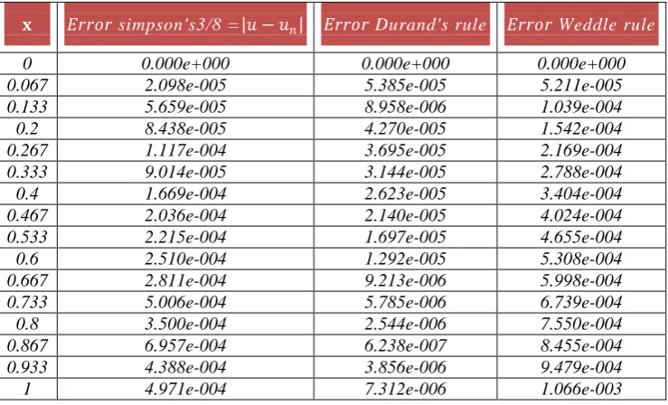
for which the exact solution is u(x) = sin(x). Tables 1.1, 1.2 and Figures 1.1, 1.2, 1.3 and 2.1, 2.2, 2.3 show that the approximation and exact solution by using Simpson's 3/8 method, Durand's method and Weddle method respectively for n= 5, 7.

Table 1.1: The Error of Example 1 by using Simpson's 3/8 rule, Durand's rule and Weddle rule respectively with n=5,7

𝐱𝐱 Error simpson's3/8 =|𝑢𝑢 − 𝑢𝑢_𝑛𝑛| Error Durand's rule Error Weddle rule

0 0.000e+000 0.000e+000 0.000e+000

0.067 2.098e-005 5.385e-005 5.211e-005

0.133 5.659e-005 8.958e-006 1.039e-004

0.2 8.438e-005 4.270e-005 1.542e-004

0.267 1.117e-004 3.695e-005 2.169e-004

0.333 9.014e-005 3.144e-005 2.788e-004

0.4 1.669e-004 2.623e-005 3.404e-004

0.467 2.036e-004 2.140e-005 4.024e-004

0.533 2.215e-004 1.697e-005 4.655e-004

0.6 2.510e-004 1.292e-005 5.308e-004

0.667 2.811e-004 9.213e-006 5.998e-004

0.733 5.006e-004 5.785e-006 6.739e-004

0.8 3.500e-004 2.544e-006 7.550e-004

0.867 6.957e-004 6.238e-007 8.455e-004

0.933 4.388e-004 3.856e-006 9.479e-004

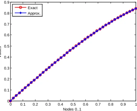
Figure 1.1: shows both the exact and the approximate Simpson's 3/8 rule with n =5

Figure 1.2: compares the exact solution u(x) =sinx with the approximate Durand's rule with n=5

Figure 1.3: compares the exact solution with the approximate Weddle solution.

0 0.1 0.2 0.3 0.4 0.5 0.6 0.7 0.8 0.9 1

0 0.1 0.2 0.3 0.4 0.5 0.6 0.7 0.8 0.9

Nodes 0..1

V

al

ues

Exact Approx.

0 0.1 0.2 0.3 0.4 0.5 0.6 0.7 0.8 0.9 1

0 0.1 0.2 0.3 0.4 0.5 0.6 0.7 0.8 0.9

Nodes 0..1

V

al

ues

Exact Approx.

0 0.1 0.2 0.3 0.4 0.5 0.6 0.7 0.8 0.9 1

0 0.1 0.2 0.3 0.4 0.5 0.6 0.7 0.8 0.9

Nodes 0..1

V

al

ues

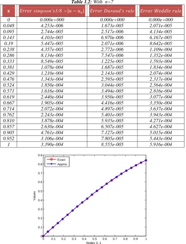
Table 1.2: With n=7

𝐱𝐱 Error simpson's3/8 =|𝑢𝑢 − 𝑢𝑢_𝑛𝑛| Error Durand's rule Error Weddle rule

0 0.000e+000 0.000e+000 0.000e+000

0.048 4.253e-006 1.673e-005 2.071e-005

0.095 2.744e-005 2.517e-006 4.134e-005

0.143 4.103e-005 6.970e-006 6.167e-005

0.19 5.447e-005 2.071e-006 8.642e-005

0.238 4.357e-005 2.772e-006 1.109e-004

0.286 8.134e-005 7.547e-006 1.352e-004

0.333 8.549e-005 1.225e-005 1.593e-004

0.381 1.078e-004 1.687e-005 1.834e-004

0.429 1.210e-004 2.143e-005 2.074e-004

0.476 1.343e-004 2.595e-005 2.317e-004

0.524 1.850e-004 3.044e-005 2.564e-004

0.571 1.616e-004 3.494e-005 2.816e-004

0.619 2.440e-004 3.950e-005 3.077e-004

0.667 1.905e-004 4.416e-005 3.350e-004

0.714 2.072e-004 4.897e-005 3.637e-004

0.762 2.243e-004 5.401e-005 3.943e-004

0.810 3.878e-004 5.935e-005 4.271e-004

0.857 2.630e-004 6.507e-005 4.627e-004

0.905 4.761e-004 7.127e-005 5.015e-004

0.952 3.106e-004 7.805e-005 5.443e-004

1 3.390e-004 8.555e-005 5.916e-004

Figure 2.1: compares the exact solution u(x) = sinx with the approximate Simpson's 3/8 solution with n=7

0 0.1 0.2 0.3 0.4 0.5 0.6 0.7 0.8 0.9 1

0 0.1 0.2 0.3 0.4 0.5 0.6 0.7 0.8 0.9

Nodes 0..1

V

al

ues

Exact Approx.

0 0.1 0.2 0.3 0.4 0.5 0.6 0.7 0.8 0.9 1

0 0.1 0.2 0.3 0.4 0.5 0.6 0.7 0.8 0.9

Nodes 0..1

V

al

ues

Figure 2.3: shows the exact solution u(x)= sinx with the approximate Weddle solution when n= 7.

CONCLUSIONS

Which obtain from the illustrative example, we conclude that:

1. The proposed numerical methods are efficient and accurate to estimate the solution of these equations.

2. In most cases, the (LMVFIE's) are usually difficult to solve analytically, so we can solved by approximation method.

3. In this work the tables are appointed the common points of comparison between the three methods. 4. The Durand's method gives better accuracy than other methods.

5. When n increase, we notice the values h decrease and the error decrease. 6. This methods can be applied to nonlinear (MVFIE’s).

REFERENCES

1. Changqing Y., Jianhua H. ''Numerical Method For Solving Volterra Integral Equations with a Convolution Kernel'', IJAM, Vol. 43, No. 4, (2013).

2. Jerri A.J., "Introduction to Integral Equations with Applications", Marcel Dekker, INC, New York and Bassel, (1985).

3. Abdul-Majid Wazwaz, ''Linear and Non-Linear Integral Equations’’ Springer Heidelberg, Dordrechi London, (2011).

4. Muna M. and Iman N. '' Numerical Solution of Linear Volterra-Fredholm Integral Equations Using Lagrange Polynomials'', Mathematical Theoryand Modeling, Vol.4, No.5, p.p. 2224-5804, (2014).

5. Hendi F. and Bakodah, '' Numerical Solution of Fredholm- Volterra Integral Equation in Two Dimensional Space By Using Discrete Adomain Decomposition Method'', IJRRAS , Vol.10, No.3, (2014).

6. Majeed S. and Omran H. ''Numerical Methods for Solving Linear Volterra-Fredholm Integral Equations''; Journal of Al- Nahrain University, Vol.11 (3), p.p. 131-134, (2008).

7. Omran H., '' Numerical method for solving the first order linear Fredholm-Volterra integro-differential equations; Journal of Al- Nahrain University, Vol.12 (3), pp.139-143, (2009).

8. Maleknejad K. and Mahdiani K., ''Solution and Error Analysis of Two Dimensional Fredholm-Volterra Integral Equations Using PiecewiseConstant Functions''; j.ajcam, Vol. 2(1), p.p. 53-57, (2012).

9. Hendi F. and Albugami A.,''Numerical solution for Fredholm–Volterra integral equation of the second kind by using collocation and Galerkin methods''; Journal of King Saud University, Vol. 22, p.p. 37–40, (2009). 10. Prem K. Kythe and Pratap Puri. “Computational Methods for Linear Integral Equations'', Springer

Science+Business Media New- York, (2002).

Source of support: Nil, Conflict of interest: None Declared

[Copy right © 2015. This is an Open Access article distributed under the terms of the International Journal of Mathematical Archive (IJMA), which permits unrestricted use, distribution, and reproduction in any

medium, provided the original work is properly cited.]

0 0.1 0.2 0.3 0.4 0.5 0.6 0.7 0.8 0.9 1

0 0.1 0.2 0.3 0.4 0.5 0.6 0.7 0.8 0.9

Nodes 0..1

V

al

ues