Proceedings of the
Tenth International Workshop on
Graph Transformation and
Visual Modeling Techniques
(GTVMT 2011)
Treewidth, Pathwidth and Cospan Decompositions
Christoph Blume, H. J. Sander Bruggink, Martin Friedrich and Barbara K¨onig
13 pages
Guest Editors: Fabio Gadducci, Leonardo Mariani
Managing Editors: Tiziana Margaria, Julia Padberg, Gabriele Taentzer
Treewidth, Pathwidth and Cospan Decompositions
Christoph Blume, H. J. Sander Bruggink, Martin Friedrich and Barbara K¨onig∗
Universit¨at Duisburg-Essen, Germany
[email protected],[email protected],[email protected], barbara [email protected]
Abstract:We will revisit the categorical notion of cospan decompositions of graphs and compare it to the well-known notions of path decomposition and tree decompo-sition from graph theory. More specifically, we will define several types of cospan decompositions with appropriate width measures and show that these width measures coincide with pathwidth and treewidth. Such graph decompositions of small width are used to efficiently decide graph properties, for instance via graph automata.
Keywords:cospans, graph decompositions, pathwidth, treewidth
1
Introduction
In graph rewriting the notion of cospan plays a major role: cospans can be seen as graphs equipped with an inner and an outer interface and they can be used as (atomic) building blocks for constructing or decomposing larger graphs. Furthermore cospans are a means to cast graph rewriting into the setting of reactive systems [LM00,SS05].
In graph theory there are different notions for decomposing graphs: path and tree decomposition [RS86], which at first glance seem to have a very different flavour. These notions lead to width measures such as pathwidth and treewidth and they are used to specify how similar a graph is to a path or a tree. Treewidth plays a major role in complexity theory: for instance Courcelle’s theorem [Cou90] states that every graph property that can be specified in monadic second-order graph logic can be checked in linear time on graphs of bounded treewidth. Furthermore there are intuitive game characterizations (robber and cops games) for treewidth.
In this paper we show that, when seen from the right angle, graph decompositions based on cospans are in fact very similar to path and tree decompositions. In order to be able to state this formally we classify several types of cospan decompositions, which are sequences of cospans (with varying additional conditions). Obtaining the decomposed graph amounts to taking the colimit of the resulting diagram. We define width measures based on such decompositions and show that the width measures all coincide with pathwidth. In the second part of the paper the results are repeated for tree-like decompositions and treewidth, where the tree-like compositions are trees where the edges are labeled with spans or cospans, and the decomposed graph is again obtained by taking the colimit.
Our interest in this area stems from our work on recognizable graph languages [BK08], which in [BBK10] were used to check invariants of graph transformation systems. In this context we proposed automaton functors as an automaton model for accepting graph languages. Automaton
∗This work is supported by the
functors work by decomposing a graph into a sequence of smaller graphs with interfaces (formally cospans in the category of graphs, and therefore such sequences are called cospan decompositions), and then running a finite automaton on the sequence. This approach is an extension of the work by Courcelle and others on recognizable graph languages [Cou90], which are equivalent to the notion of inductive graph properties [HKL93].
In order to represent such structures in a computer, the interface size of the decompositions must be bounded. We suspected for some time that this bound was strongly related to the notion of pathwidth, but the relation was never formally investigated.
As far as we know there have been only few investigations into the notions of pathwidth and treewidth in the context of graph rewriting. We are mainly aware of the relation between context-free (or hyperedge replacement) grammars and bounded treewidth that is discussed in [Hab92,Lau88,Lau91]. It is shown that the language generated by a context-free grammar has always bounded treewidth, that is, there is an upper bound for the treewidth of every graph in the language. This also implies the well-known result that the language of all graphs is not context-free.
Interest in the relation between tree decompositions and graph rewriting seems to have declined since, but in our opinion this area has a lot of potential for an increased interaction of graph transformation and graph theory, since graph decompositions and width measures are still of central interest to the graph theory community. As far as we are aware of, the relation between cospan decompositions and tree and path decompositions has never been formally investigated and while the main ideas are fairly straightforward it turns out that there are some subtle issues to consider when translating one representation into the other. For instance, we found that there is more than one possible translation and more than one width measure.
InSection 2we will introduce the preliminaries such as cospans and graph decompositions. Then inSection 3we will have a closer look at cospans, identifying also atomic cospans as building blocks. Then inSection 4we will compare cospan decompositions with path decompositions and inSection 5with tree decompositions. Finally we will conclude withSection 6. The proofs can be found in the full version of this paper [BBFK11].
2
Preliminaries
ByNk we denote the set{1, . . . ,k}. The set of finite sequences over a set Ais denotedA∗. If
f:A→Bis a function fromAtoB, we will implicitly extend it to subsets and sequences; for
A0⊆Aand~a=a1. . .an∈A∗: f(A0) ={f(a)|a∈A0}and f(~a) = f(a1). . .f(an).
2.1 Categories and Cospans
We presuppose a basic knowledge of category theory. For an arrow f fromA toBwe write
f: A→B and definedom(f) =Aand cod(f) =B. For arrows f: A→B andg:B→C, the composition of f and gis denoted(f ;g):A→C. The categoryRelhas sets as objects and relations as arrows. Its subcategorySethas only the functional relations (functions) as arrows.
Aspanin a categoryCis a pairhcL,cRiofC-arrowsG cL−I−cRH. The dual notion to
hcL,cRiofC-arrowsJ−cLG cR−K. Composition of two cospanshcL,cRi,hdL,dRiis computed
by taking the pushout of the arrowscRanddL.
Cospans (and spans) are isomorphic if their middle objects are isomorphic (such that the isomorphism commutes with the component morphisms of the cospan). Isomorphism classes of cospans are the arrows of so-called cospan categories. That is, for a categoryCwith pushouts, the categoryCospan(C)has the same objects asC. The isomorphism class of a cospanc:J−cL
G cR−KinCis an arrow fromJtoKinCospan(C)and will be denoted byc:J#K.
Colimits can be seen as “generalized” pushouts. Given a collection (diagram)Dof objects {A1, . . . ,An}and morphisms between them, thecolimit of Dis an objectBtogether with
mor-phisms fi:Ai→Bsuch that the diagram commutes, and for objectsB0and morphisms fi0:Ai→B0
where the diagram commutes, it holds that there exists a uniqueh:B→B0such that the diagram commutes. We will writeColim(D) =Bin this case (where we allowDto be any representation of a diagram, for example a sequence).
2.2 Graphs and Decompositions
Ahypergraphover a set of labelsΣ(in the following also simply called graph) is a structure
G=hV,E,att,labi, whereV is a finite set of nodes,Eis a finite set of edges,att:E→V∗maps each edge to a finite sequence of nodes attached to it, andlab:E→Σassigns a label to each
edge. The size of the graphG, denoted|G|, is defined to be the cardinality of its node set, that is|G|=|V|. Adiscrete graphis a graph without edges; the discrete graph with node setNkis
denoted byDk. We denote theempty graphby /0 instead ofD0.
A graph morphism is a structure preserving map between two graphs. The category of graphs and graph morphisms is denoted by Graph. Recall, that the monomorphisms (monos) and
epimorphisms(epis) of the categoryGraphare the injective and surjective graph morphisms, respectively.
A cospanJ−cLG cR−KinGraphcan be viewed as a graph (G) with two interfaces (Jand
K), called theinner interfaceandouter interfacerespectively. Informally said, only elements of
Gwhich are in the image of one of the interfaces can be “touched”. By[G]we denote the trivial cospan /0→G← /0, the graphGwith two empty interfaces.
For the use in definitions we define a second kind graph. Asimple graphis a tuplehV,Eiwhere
V is a finite set of nodes andE⊆ {{t1,t2} |t1,t2∈V,t16=t2}the set of edges.1 Atreeis a simple graph in which there exists exactly one path between each pair of nodes. Apath graph2is a tree in which each node is connected to either one or two other nodes. Simple graphs, and in particular trees and path graphs, are only used to define tree and path decompositions. All objects we are decomposing will be hypergraphs.
Definition 1 LetG=hV,E,att,labibe a graph. Atree decompositionofGis a pairT =hT,Xi, whereT is a tree andX={Xt1, . . . ,Xtn}is a family of subsets ofV (which are calledbagsin the
literature) indexed by the nodes ofT, such that:
– for each nodev∈V, there exists a nodetofT such thatv∈Xt;
1In the following,v,wwill range over nodes of hypergraphs,eover edges of hypergraphs,tover nodes of simple graphs andbover edges of simple graphs. In all cases, subscripts may also be used.
1
2 3 4
(a) GraphGP
1
2 3
3 4
(b) Path Decomposition ofGP
Figure 1: The graphGP and one of its path decompositions
1
2 3 4 5 6
7 8
9 10
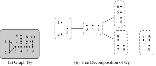
(a) GraphGT
1
2 3
3 4 7
4 5 6
7 8
9
8
9 10
(b) Tree Decomposition ofGT
Figure 2: The graphGT and one of its tree decompositions
– for each edgee∈E, there is a nodetofT such that all nodesvconnected toeare inXt;
– for each nodev∈V, the simple graph induced by the nodes{t|v∈Xt}is a subtree ofT.
The width of a tree decompositionT =hT,Xiiswd(T) = maxt∈T|Xt|
−1. A tree decomposi-tionT =hT,Xiis apath decompositionifT is in fact a path graph.
Now, the pathwidth pwd(G)and the treewidthtwd(G)of a graphGare defined as follows: – pwd(G) =min{wd(P)| Pis a path decomposition ofG},
– twd(G) =min{wd(T)| T is a tree decomposition ofG}.
Example1 As examples we consider only unlabeled directed graphs, that is we takeΣ={?}as alphabet and|att(e)|=2for every edgee. LetGPbe the graph shown inFigure 1a. Obviously,
the pathwidth of this graph is at least2since it contains a 3-clique (all nodes of which have to be together in at least one bag) and we have a path decompositionP of width2which is shown in
Figure 1b.
As an example for a tree decomposition we consider the unlabeled graphGT ofFigure 2a. The
treewidth of this graph is2due to the fact that it contains a3-clique and that the tree decomposition
T shown inFigure 2bhas width2.
3
Cospans as Building Blocks for Graphs
Cospans of graphs can be viewed as operations on graphs with interfaces (in the sense of Courcelle [Cou90,BC87]). LetGbe a graph with external nodes (which itself can be represented by a cospang: /0→G←I, where the interfaceI represents the external nodes) andc: I→H←K
a cospan. By composinggandc we obtain a cospan(g;c): /0→GH←K, whereGHis the pushout object ofG←I→H. Recall, that taking a pushout in the category of graphs amounts to constructing the disjoint union ofGandH, and subsequently fusing just enough nodes to make the pushout diagram commute. That is, by composing with a cospan we canaddnew nodes,fuse
existing nodes andchangethe interface of a graph.
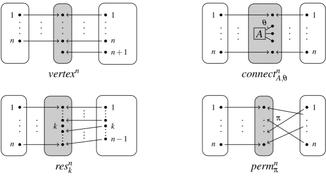
There exist finite sets of cospans (calledatomic cospans) from which, together with disjoint union, all graphs with interfaces can be built; see for example [GH97] and [BK06]. Since we do not have disjoint union, we have to settle for finitely many atomic cospansper pair of inner and outer interface(of which there are infinitely many). Here, we use the following atomic cospans. Letn∈Nbe the size of the inner interface.
– Add a node: vertexn:Dn#Dn+1. This cospan is defined as
vertexn=Dn id0
−→Dn+1
id
←−Dn+1, whereid0(x) =xforx≤n.
– Remove a node from the interface: resnk: Dn#Dn−1, wheren≥1 and 1≤k≤n. This cospan is defined as
resnk=Dn id
−→Dn
φ
←−Dn−1, whereφ(x) =
(
x ifx<k x+1 ifx≥k.
– Add an edge: connectnA,θ: Dn #Dn, whereA∈Σ is a label andθ:Nar(A)→Nn is a
function which specifies how the new edge is connected to the nodes in the interface. This cospan is defined as
connectnA,θ =Dn id0
−→G id
0 ←−Dn,
whereG=hV,E,att,labiwithV=Nn,E={e},att(e) =θ(1). . .θ(ar(A))andlab(e) =A;
andid0(x) =xforx≤n.
– Permute the order of the nodes in the interface:permnπ:Dn#Dn. This cospan is defined as
permnπ=Dn id
−→Dn
π ←−Dn,
whereπ:Nn→Nnis a permutation (that is, it is bijective).
The atomic cospans are graphically depicted inFigure 3.
Lemma 1 Let c=J−cLG cR−K be a cospan such that J,K are discrete and cL,cRare monos.
Then there exist atomic cospans a1, . . . ,ansuch that c=a1;· · ·;an.
Moreover, the following condition holds for this atomic cospan decomposition: Let ai=Ii−1→
1
n
1
n n+1
1
n
A
θ
1
n
vertexn connectnA,θ
1
n
k
1
k n−1
1
n
1
n
π
resnk permnπ
Figure 3: Graphical representations of the atomic cospans.
4
Path-like Decompositions: Cospan Decompositions
In this section we explore “path-like” cospan decompositions of graphs. Such decompositions are naturally defined as sequences of cospans, which are composed to a graph by taking the colimit of the emerging diagram. Equivalently, the cospans can be iteratively composed into a single cospan, where finally the interfaces are ignored.
Definition 2 LetGbe a graph and~c=c1, . . . ,cnbe a sequence of composable cospans in the
categoryGraph. The sequence~cis acospan decompositionofG, ifColim(~c) =G.
Note that we now have three related notions: cospan decompositions, which are sequences of cospans; the single cospan (“graph with interfaces”) which is the result of composing the cospans in a cospan decomposition; and the center graph of this cospan.
We consider the following types of cospan decompositions. The first two correspond to path decompositions in two different ways: in graph-bag decompositions the center graphs in the cospans correspond to the bags ofDefinition 1, whereas in interface-bag decompositions the interfaces play the role of bags. In order to make the relation between path and cospan decompositions clearer, we will only consider decompositions into cospans of injective morphisms in this paper.
Definition 3 Let~cbe a cospan decomposition of the graphG.
(i) ~c is a graph-bag decomposition, if all cospans have discrete interfaces and consist of injective morphisms.
(ii) ~cis aninterface-bag decomposition, if it is a graph-bag decomposition, consist of pairs of jointly node-surjective morphisms3and it holds for all edgeseofG, withatt(e) =v1. . .vm,
thatv1, . . . ,vmoccur together in some interface.
(iii) ~cis anatomic cospan decomposition, if it consists only of atomic cospans.
It is clear that the various types of cospan decomposition are strictly contained in one another, that is: Atomic⊂Interface-bag⊂Graph-bag⊂All.
Definition 4 Letc:J→G←Kbe a cospan. We define thegraph-bag sizeandinterface-bag sizeofcas follows:
|c|gb:=|VG|
|c|ib:=max{|VJ|,|VK|}
Observe, that for all atomic cospanscit holds that|c|gb=|c|ib. For convenience later on, we define|c|at:=|c|gb(=|c|ib).
Now we are ready to define, for all three types of cospan decomposition, awidth:
Definition 5
– Let~c=c1;· · ·;cnbe a decomposition. We define thegraph-bagandinterface-bag width
of~cas follows:
wdgb(~c):=max{|ci|gb: 1≤i≤n} −1
wdib(~c):=max{|ci|ib: 1≤i≤n} −1
– LetGbe a graph. The graph-bag (cpwdgb(~c)), interface-bag (cpwdib(~c)) and atomic cospan width (cpwdat(~c)) ofGare defined as:
cpwdgb(G):=min{wdgb(~c):~cis a graph-bag decomposition ofG}
cpwdib(G):=min{wdib(~c):~cis an interface-bag decomposition ofG}
cpwdat(G):=min{wdib(~c):~cis an atomic cospan decomposition ofG}
The main theorem of this section is that, for a given graph, the three notions of cospan pathwidth are the same, and moreover are the same as the pathwidth of the graph. First, we show how to transform (cospan) path decompositions into each other:
Lemma 2
(i) LetP be a path decomposition of a graph G. There exists a graph-bag decomposition~c of G such that wdgb(~c) =wd(P).
(ii) Let~c be a graph-bag decomposition of G. There exists an interface-bag decompositiond of~ G such that wdib(d~) =wdgb(~c).
(iii) Let~c be a graph-bag decomposition of G. There exists an atomic cospan decomposition~d of G such that wdat(~d)≤wdgb(~c).
(iv) Let~c be an interface-bag decomposition of G. There exists a path decompositionP of G such that wd(P) =wdib(~c).
/0 1
2
3 3 3 4 /0
(a) Graph-bag decomposition ofGP
1
2 3
1
2
3 3 3 4 3 4
(b) Interface-bag decomposition ofGP
Figure 4: Graph-bag and interface-bag decomposition ofGP
Example2 As an example we take the graphGPand the corresponding path decompositionP
ofExample 1. We use the path decomposition to construct a graph-bag decomposition ofGP.
For each of the two bags inP we take a cospan where the center graph of the first cospan is the 3-clique and the center graph of the second cospan contains the edge from the third to the fourth node. The inner interface of the first cospan and the outer interfaces of the second cospan are both empty graphs, while the outer interface of the first cospan (which is the inner interface of the second cospan) contains the third node which is the intersection of both subgraphs. The resulting graph-bag decomposition is depicted inFigure 4a. The graph-bag width ofGP is 2, since the
resulting graph-bag decomposition has graph-bag size 2 and the graph-bag size of every other graph-bag decomposition must have at least size 2 due to the 3-clique which has to be contained in at least one center graph.
An interface-bag decomposition for the same graph is shown inFigure 4b. Note that it indeed satisfies the conditions ofDefinition 3: specifically each cospan is jointly node-surjective and all nodes attached to an edge live together in at least one bag. The interface-bag width ofGPis 2,
due to the fact that the given interface-bag decomposition has interface-bag width 2 and any other interface-bag decomposition has to contain the nodes of the 3-clique in at least one interface.
To construct the atomic decomposition we decompose the cospans of the graph-bag decompo-sition into atomic cospans. This is possible due toLemma 1:
vertex0;vertex1;vertex2;connect3A,
θ13,2;connect
3
A,θ13,3 ;connect
3
A,θ23,3 ;res
3 0;res20;
vertex1;connect2A,
θ12,2 ;res
2 0;res10,
whereθin
1,...,im:Nm→Nndenotes the function which mapsθ(1) =i1, . . . ,θ(m) =im.
More details concerning the conversion of the various cospan decompositions into each other can be found in the proof ofLemma 2in the full version of this paper [BBFK11].
5
Tree-like Decompositions: Star and Costar Decompositions
In this section we repeat the work ofSection 4for tree-like “cospan”-decompositions. We define
starsandcostarsas generalizations of spans and cospans, respectively. A star is a finite set of morphisms with the same domain, while a costar is a finite set of morphisms with the same codomain.
of the first two relate to the form of the stars (joins) in the tree; the third one is a special case of the second. Where a cospan can be seen as a graph with two interfaces, a costar can be seen as a graph with an arbitrary number of interfaces. A costar decomposition is a decomposition into costars, where costars are connected via the interfaces in such a way that they form a tree. Note that the edges of this tree are spans. On the other hand, a star decomposition is a decomposition into stars, where the edges of the corresponding tree-like structure correspond to cospans (see alsoFigure 5). As in the case of cospan decompositions, we restrict our attention to injective morphisms.
Definition 6
(i) Acostar decompositionis a tupleC=hT,τi, whereT is a tree andτ is function which maps each nodet ofT to a graph and each edgeb={t1,t2}ofT to a span of injective morphisms
τ(b) =τ(t1)
ϕb,t1
←−−Jb
ϕb,t2
−−→τ(t2).
A costar decompositionCis a costar decompositionof GifColim(C) =G.
(ii) Astar decompositionis a tupleS=hT,τi, whereT is a tree andτ is function which maps each nodetofT to a discrete graphJand each edgeb={t1,t2}to a cospan
τ(b) =τ(t1)→Gb←τ(t2),
which consists of a pair of jointly node-surjective, injective morphisms.
A star decompositionCis a star decompositionof GifColim(C) =Gand additionally it holds for all edgeseofG, withatt(e) =v1. . .vm, thatv1, . . . ,vmoccur together inτ(t)for
somet∈VT.
(iii) Anatomic star decompositionis a star decompositionhT,τisuch thatτ(b)is an atomic cospan for all edgesbofT.
In the case of cospan decompositions we had a clear hierarchy of the various decomposition types. In the case of tree-like decompositions, however, this is not the case: the sets of star and costar decompositions are not related with respect to inclusion. (However, by definition, each atomic star decomposition is also a star decomposition.)
Definition 7 LetS=hT,τibe a costar decomposition or a star decomposition. The width ofS is defined as
wd?(S) =max
v∈VT
|τ(v)| −1.
Definition 8 Let Gbe a graph. The costar width (ctwdco?(G)), star width(ctwd?(G)) and
atomic star width(ctwdat?(F)) ofGare defined as follows:
ctwdco?(G) =min{wd?(C)| Cis a costar decomposition ofG}
ctwd?(G) =min{wd?(S)| Sis a star decomposition ofG}
ctwdat?(G) =min{wd?(S)| Sis an atomic star decomposition ofG}
As in the previous section, the various notions defined in this section are equivalent to the notion of treewidth.
Lemma 3
(i) LetT be a tree decomposition of G. There exists a star decompositionS of G such that wd?(S) =wd(T).
(ii) LetSbe a star decomposition of G. There exists a costar decompositionCof G such that wd?(C) =wd?(S).
(iii) LetCbe a costar decomposition of G. There exists a tree decompositionT of G such that wd(T) =wd?(C).
(iv) LetS be a star decomposition of G. There exists an atomic star decompositionS0 of G
such that wd?(S0) =wd?(S).
Theorem 2 For every graph G, twd(G) =ctwdco?(G) =ctwd?(G) =ctwdat?(G).
Example3 We consider the graphGT and the tree decompositionT ofExample 1. In order to
construct a star decomposition ofGT, we take a cospan for each of the four edges (of the tree) of
T. The interfaces of these four cospans are the discrete graphs corresponding to the bags. The center graph of each cospan is the subgraph containing the nodes of both the inner and the outer interface of the cospan and (possibly) edges connecting these nodes. It has to be ensured that each edge occurs exactly once. This leads to the star decomposition shown inFigure 5a. Since the width of the given star decomposition has size 2 and the nodes of the 3-clique has to be contained together in at least one interface of any star decomposition, the star width ofGT is 2.
The costar decomposition can be obtained from the star decomposition. Each of the four cospans of the star decomposition is converted into a span. The inner and the outer graph of each span contain the nodes of the corresponding cospan interfaces plus additional edges. (Note that due to the conditions on star decompositions, each edge can be “shifted” into at least one interface.) The center graph of the span is then the discrete graph obtained by the intersection of the inner and the outer graphs of the span. The resulting costar decomposition is shown in
Figure 5b. The costar width ofGT is 2 due to the fact that the given costar decomposition has size
2 and that any costar decomposition must contain the 3-clique in some graph of at least one span. More details concerning the conversion of the various tree and star decompositions into each other can be found in the proof ofLemma 2in the full version of this paper [BBFK11].
6
Conclusion
1
2 3 1
2 3 4 7
3 4 7
3 4 5 6 7 4 5 6
3 4 7 8 9 7 8 9 7 8 9 10 8 9 10
(a) Star decomposition ofGT
1
2 3
3 3 4 7 4 4 5 6 7 7 8 9 8 9 8 9 10
(b) Costar decomposition ofGT
Figure 5: Star and costar decomposition ofGT
there are indeed several possible choices, mainly depending on whether we identify bags with interfaces or with the center graph in a cospan. Furthermore there is in addition the notion of decomposition into atomic cospans, which can be viewed as atomic building blocks. The investigations in this paper have their origin in a Master’s thesis [Fri10].
Since the notion of tree decomposition and treewidth has many applications in graph theory, we expect that some of these applications are also useful in a more graph transformation oriented setting. We are specifically interested in using path and tree decompositions for recognizable graph languages [Cou90] or – more specifically – for graph automata acting as acceptors of graph languages. In order to accept a graph, it is decomposed into atomic units and read – step by step – by the automaton. Depending on whether the state of the automaton, after reading the entire graph, is final, the graph is accepted. In general, decompositions of arbitrary width must be considered, which leads to graph automata with an infinite number of states. For implementation purposes, we have to restrict the width of the considered decompositions – and thus the path width of the accepted graphs – in order to obtain automata with a finite state set. The size of the state set, however, appears to grow exponentially in the size of the considered maximum width. Therefore we are interested in path and tree decompositions of moderate size, so that graph automata can be implemented efficiently.
Tree automata have already been used for similar purposes in [CD10,GPW10].
Finally, let us remark that we did not treat the question of howto obtain such path or tree decompositions, given a single, monolithic graph. This is a non-trivial problem that has been studied by Bodlaender et al. [Bod96,BK96]. It can be shown that for a fixed parameterkit can be checked in linear time (in the size of the graph), whether the given graph has pathwidth or treewidth smaller thank. Furthermore the respective decompositions can be obtained in linear time. However, despite their good runtime behaviour in theory, these algorithms are not really practical (see also the investigations in [K¨up10]), which means that heuristics are used in practice.
Acknowledgements. We thank the anonymous referees for their valuable remarks about the
submitted version of this paper.
Bibliography
[BBFK11] C. Blume, S. Bruggink, M. Friedrich, B. K¨onig. Treewidth, Pathwidth and Cospan Decompositions. Technical report, Abteilung f¨ur Informatik und angewandte Kogni-tionswissenschaften, Universit¨at Duisburg-Essen, 2011.
[BBK10] C. Blume, S. Bruggink, B. K¨onig. Recognizable Graph Languages for Checking Invariants. InProc. of GT-VMC 2010. 2010.
[BC87] M. Bauderon, B. Courcelle. Graph Expressions and Graph Rewritings.Mathematical Systems Theory20:83–127, 1987.
[BK96] H. L. Bodlaender, T. Kloks. Efficient and constructive algorithms for the pathwidth and treewidth of graphs.Journal of Algorithms21(2):358–402, 1996.
[BK06] S. Bozapalidis, A. Kalampakas. Recognizability of graph and pattern languages.Acta Informatica42(8/9):553–581, 2006.
[BK08] S. Bruggink, B. K¨onig. On the Recognizability of Arrow and Graph Languages. In
Proc. of ICGT ’08. Springer, 2008. LNCS 5214.
[Bod96] H. L. Bodlaender. A Linear Time Algorithm for Finding Tree-Decompositions of Small Treewidth.SIAM J. Comput.25(6):1305–1317, 1996.
[CD10] B. Courcelle, I. Durand. Verifying monadic second order graph properties with tree automata. InEuropean Lisp Symposium. May 2010.
[CDG+] H. Comon, M. Dauchet, R. Gilleron, C. L¨oding, F. Jacquemard, D. Lugiez, S. Tison, M. Tommasi. Tree Automata Techniques and Applications. Available from: http: //www.grappa.univ-lille3.fr/tata. 12 October 2007.
[Fri10] M. Friedrich. Baumautomaten und Baumzerlegungen f¨ur erkennbare Graphsprachen. Master’s thesis, Universit¨at Duisburg-Essen, July 2010.
[GH97] F. Gadducci, R. Heckel. An inductive view of graph transformation. InProceedings of WADT ’97. Pp. 223–237. 1997.
[GPW10] G. Gottlob, R. Pichler, F. Wei. Bounded treewidth as a key to tractability of knowledge representation and reasoning.Journal of Artificial Intelligence174(1):105–132, 2010.
[Hab92] A. Habel. Hyperedge Replacement: Grammars and Languages. Springer-Verlag, 1992. LNCS 643.
[HKL93] A. Habel, H.-J. Kreowski, C. Lautemann. A comparison of compatible, finite, and inductive graph properties.Theoretical Computer Science110(1):145–168, 1993.
[K¨up10] S. K¨upper. Algorithmen f¨ur Baum- und Pfadzerlegungen von Graphen. Bachelor’s thesis, Universit¨at Duisburg-Essen, October 2010.
[Lau88] C. Lautemann. Decomposition Trees: Structured Graph Representation and Efficient Algorithms. InProc. of CAAP ’88. Pp. 28–39. Springer, 1988. LNCS 299.
[Lau91] C. Lautemann. Tree Automata, Tree Decomposition and Hyperedge Replacement. In
Proc. of Graph-Grammars and Their Application to Computer Science ’90. Pp. 520– 537. Springer, 1991. LNCS 532.
[LM00] J. J. Leifer, R. Milner. Deriving Bisimulation Congruences for Reactive Systems. In
Proc. of CONCUR 2000. Pp. 243–258. Springer, 2000. LNCS 1877.
[RS86] N. Robertson, P. Seymour. Graph minors. II. Algorithmic aspects of tree width.
Journal of Algorithms7:309–322, 1986.