Lecture Notes

Lecture Notes 14

36-705

We continue with our discussion of decision theory.

1

Decision Theory

Suppose we want to estimate a parameter θ using data Xn _{= (X1, . . . , Xn). What is the} best possible estimator θb= θ(X1, . . . , Xn) ofb θ? Decision theory provides a framework for answering this question.

1.1

The Risk Function

Let θb= θ(Xb n_{) be an estimator for the parameter θ ∈ Θ. We start with a loss function} L(θ,θ) that measures how good the estimator is. For example:b

L(θ,θ) = (θb −θ)b2 _{squared error loss,} L(θ,θ) =b |θ−bθ| absolute error loss, L(θ,θ) =b |θ−bθ|p _{Lp loss,}

L(θ,θ) = 0 ifb θ =θbor 1 if θ 6=bθ zero–one loss, L(θ,θ) =b I(|θb−θ|> c) large deviation loss, L(θ,θ) =b R logp(x;θ)

p(x;θ)b

p(x;θ)dx Kullback–Leibler loss. If θ= (θ1, . . . , θk) is a vector then some common loss functions are

L(θ,bθ) = kθ−θbk2 = k

X

j=1

(θjb −θj)2,

L(θ,θ) =b kθ−θbkp = k

X

j=1

|θjb −θj|p

!1/p .

When the problem is to predict a Y ∈ {0,1} based on some classifierh(x) a commonly used loss is

L(Y, h(X)) =I(Y 6=h(X)). For real valued prediction a common loss function is

0 1 2 3 4 5 0

1 2 3

R(θ,θ1)b R(θ,θb2)

θ

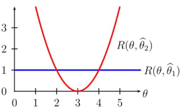
Figure 1: Comparing two risk functions. Neither risk function dominates the other at all values of θ.

The risk of an estimator θbis R(θ,θ) =b Eθ

L(θ,bθ)

=

Z

L(θ,θ(x1, . . . , xn))p(x1, . . . , xn;b θ)dx. (1)

When the loss function is squared error, the risk is just the MSE (mean squared error): R(θ,θ) =b Eθ(θb−θ)2 =Varθ(θ) + biasb 2. (2) If we do not state what loss function we are using, assume the loss function is squared error.

1.2

Comparing Risk Functions

To compare two estimators, we compare their risk functions. However, this does not provide a clear answer as to which estimator is better. Consider the following examples.

Example 1 Let X ∼ N(θ,1) and assume we are using squared error loss. Consider two estimators: bθ1 = X and θ2b = 3. The risk functions are R(θ,θ1) =b Eθ(X −θ)2 _{= 1 and} R(θ,θ2) =b Eθ(3−θ)2 = (3−θ)2. If 2< θ <4 then R(θ,θ2)b < R(θ,θ1)b , otherwise, R(θ,θ1b)< R(θ,θ2)b . Neither estimator uniformly dominates the other; see Figure 1.

Example 2 Let X1, . . . , Xn ∼ Bernoulli(p). Consider squared error loss and let p1_b = X. Since this has zero bias, we have that

R(p,p1) =_b Var(X) = p(1−p)

n .

Another estimator is

b

p2 = Y +α α+β+n

where Y =Pn_i=1Xi and α and β are positive constants.1 Now,

R(p,p2) =b Varp(p2) + (biasp(b p2))b 2

= Varp

Y +α α+β+n

+

Ep

Y +α α+β+n

−p

2

= np(1−p) (α+β+n)2 +

np+α α+β+n −p

2 .

Let α =β =pn/4. The resulting estimator is

b

p2 = Y +

p

n/4 n+√n

and the risk function is

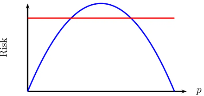
R(p,bp2) = n 4(n+√n)2.

The risk functions are plotted in Figure 2. As we can see, neither estimator uniformly dominates the other.

These examples highlight the need to be able to compare risk functions. To do so, we need a one-number summary of the risk function. Two such summaries are the maximum risk and the Bayes risk.

The maximum risk is

R(θ) = supb θ∈Θ

R(θ,θ)b (3)

and theBayes risk under prior π is Bπ(θ) =b

Z

R(θ,θ)π(θ)dθ.b (4)

Example 3 Consider again the two estimators in Example 2. We have

R(p1) = max_b 0≤p≤1

p(1−p)

n =

1 4n

R

isk

p

Figure 2: Risk functions for p1_b and p2_b in Example 2. The solid curve is R(p1). The dotted_b line is R(p2).b

and

R(p2) = maxb

p

n

4(n+√n)2 =

n 4(n+√n)2.

Based on maximum risk, p2_b is a better estimator since R(p2)b < R(bp1). However, when n is large, R(p1)_b has smaller risk except for a small region in the parameter space near p= 1/2. Thus, many people prefer _bp1 to p2_b. This illustrates that one-number summaries like the maximum risk are imperfect.

These two summaries of the risk function suggest two different methods for devising estima-tors: choosing θbto minimize the maximum risk leads to minimax estimators; choosing θbto minimize the Bayes risk leads to Bayes estimators.

An estimator θbthat minimizes the Bayes risk is called a Bayes estimator. That is, Bπ(bθ) = inf

˜ θ

Bπ(˜θ) (5)

where the infimum is over all estimators ˜θ. An estimator that minimizes the maximum risk is called a minimax estimator. That is,

sup θ

R(θ,bθ) = inf ˜ θ

sup θ

R(θ,θ)˜ (6)

where the infimum is over all estimators ˜θ. We call the right hand side of (6), namely, Rn≡Rn(Θ) = inf

b

θ sup θ∈Θ

the minimax risk. Statistical decision theory has two main goals: determine the minimax risk Rn and find an estimator that achieves this risk.

Once we have found the minimax risk Rn we want to find the minimax estimator that achieves this risk:

sup θ∈Θ

R(θ,θ) = infb

b

θ sup θ∈Θ

R(θ,θ).b (8)

1.3

Bayes Estimators

Letπ be a prior distribution. After observingXn_{= (X1, . . . , Xn), the posterior distribution} is, according to Bayes’ theorem,

P(θ ∈A|Xn) =

R

Ap(X1, . . . , Xn|θ)π(θ)dθ

R

Θp(X1, . . . , Xn|θ)π(θ)dθ =

R

AL(θ)π(θ)dθ

R

ΘL(θ)π(θ)dθ

(9) where L(θ) =p(xn_{;θ) is the likelihood function. The posterior has density}

π(θ|xn_{) =} p(xn|θ)π(θ)

m(xn₎ (10)

wherem(xn_{) =}R _p(xn_{|θ)π(θ)dθ is themarginal distributionofX}n_{. Define theposterior} risk of an estimator θ(xb n_{) by}

r(θb|xn_{) =}

Z

L(θ,θ(xb n_))π(θ|xn_{)dθ. (11)}

Theorem 4 The Bayes risk Bπ(bθ) satisfies

Bπ(θ) =b

Z

r(θb|xn_)m(xn_)dxn_{. (12)}

Let θ(xb n_{) be the value of θ that minimizes r(θ}b_|xn_{). Then θ}b_{is the Bayes estimator.} Proof:

Letp(x, θ) = p(x|θ)π(θ) denote the joint density of X and θ. We can rewrite the Bayes risk as follows:

Bπ(bθ) =

Z

R(θ,θ)π(θ)dθb =

Z Z

L(θ,bθ(xn))p(x|θ)dxn

!

π(θ)dθ =

Z Z

L(θ,θ(xb n_{))p(x, θ)dx}n_{dθ =}

Z Z

L(θ,θ(xb n_))π(θ|xn_)m(xn_)dxn_dθ =

Z Z

L(θ,θ(xb n_))π(θ|xn_)dθ

!

m(xn_)dxn ₌

Z

If we choose θ(xb n_{) to be the value of θ that minimizes r(θ}b_|xn_{) then we will minimize the} integrand at every x and thus minimize the integral R r(θb|xn_)m(xn_)dxn_.

Now we can find an explicit formula for the Bayes estimator for some specific loss functions.

Theorem 5 If L(θ,θ) = (θb −bθ)2 _{then the Bayes estimator is}

b

θ(xn_{) =}

Z

θπ(θ|xn_{)dθ =}

E(θ|X =xn). (13)

If L(θ,θ) =b |θ−θb| then the Bayes estimator is the median of the posteriorπ(θ|xn_{). If L(θ,}b_θ)

is zero–one loss, then the Bayes estimator is the mode of the posterior π(θ|xn_).

Proof:

We will prove the theorem for squared error loss. The Bayes estimator θ(xb n_{) minimizes} r(θb|xn_{) =} R_(θ−θ(xb n₎₎2_π(θ|xn_{)dθ. Taking the derivative ofr(θ}b_|xn_{) with respect toθ(x}b n_{) and} setting it equal to zero yields the equation 2R(θ−θ(xb n_))π(θ|xn_{)dθ = 0. Solving for θ(x}b n₎ we get 13.

Example 6 Let X1, . . . , Xn ∼N(µ, σ2_{) whereσ}2 _{is known. Suppose we use aN(a, b}2_)prior

forµ. The Bayes estimator with respect to squared error loss is the posterior mean, which is

b

θ(X1, . . . , Xn) = b 2

b2₊σ2

n X+

σ2

n b2₊σ2

n

a. (14)

It is worth keeping in mind the trade-off: Bayes estimators although easy to compute are very subjective; they depend strongly on the prior π. Minimax estimators, although more challenging to compute are not subjective, but do have the drawback that they are protecting against the worst-case which might lead to pessimistic conclusions.

2

Minimax Estimators through Bayes Estimators

Our goal is to compute a minimax estimator θbthat satisfies: sup

θ∈Θ

R(θ,θ)b ≤inf

e

θ sup θ∈Θ

R(θ,θ).e We will let θminimax denote a minimax estimator.

2.1

Bounding the Minimax Risk

One strategy to find the minimax estimator is by finding (upper and lower) bounds on the minimax risk that match. Then the estimator that achieves the upper bound is a minimax estimator.

Upper bounding the minimax risk is straightforward. Given an estimatorθbupwe can compute its maximum risk and use it to upper bound the minimax risk, i.e.

inf

e

θ sup θ∈Θ

R(θ,θ)e ≤R(θ,θup).b

The Bayes risk of the Bayes estimator for any priorπ lower bounds the minimax risk. Fix a prior π and suppose that bθlow is the Bayes estimator with respect to π, then we have that:

Bπ(θlow)b ≤Bπ(θminimax)≤sup θ

R(θ, θminimax) = inf

e

θ sup θ∈Θ

R(θ,θ).e Let us see an example of this in action.

Example: We will prove a classical result that if we observe independent draws from a d-dimensional Gaussian, X1, . . . , Xn∼N(θ, Id), then the average:

b

θ= 1 n

n

X

i=1 Xi,

is a minimax estimator of θ with respect to the squared loss.

Let Rn denote the minimax risk. First, let us compute the upper bound on Rn. We note that,

b

θ ∼N(θ, Id/n), so that its risk:

R(θ,θ) =b E[ d

X

i=1

(θib −θi)2] =E[ d

X

i=1 Zi2], where Zi ∼N(0,1/n). This yields that,

inf

e

θ sup θ∈Θ

R(θ,θ)e ≤R(θ,θ) =b d n.

Now we lower bound the minimax risk using the Bayes risk. Let us take the prior to be zero-mean Gaussian, i.e. we take π = N(0, c2_{Id). By sufficiency, we can replace the data} with θ. We can write:b

θ ∼N(0, c2Id)

b

We can write this as

θ=c

b

θ= √1

n Z where , Z ∼N(0, Id). Hence,

θ b θ ∼N 0 0 ,

c2_{Id c}2_Id c2_{Id (c}2_{+ 1/n)Id}

We can now compute the posterior (using standard conditional Gaussian formulae), and obtain its mean:

E[θ|θ] =b c 2

c2 _{+ 1/n}θ.b Now,

R(θ,θ) =b E

c 2

c2_{+ 1/n}θb−θ

2 . Write θb=θ+W, where W ∼N(0, Id/n). Then

R(θ,θ) =b EW

c 2

c2_{+ 1/n}Z−

θ n(c2 _{+ 1/n)}

2 . Let us denote β:=c2_{+ 1/n. Then we obtain that,}

R(θ,θ) =b kθk 2 2 n2_β2 +

c4

β2EkWk 2 2 =

kθk2 2 n2_β2 +

c4 β2

d n. The Bayes risk further averages this over θ∼N(0, c2_{Id) to obtain that,}

Bπ

c2 c2 _{+ 1/n}θb

= c 2_d n2_β2 +

c4 β2

d n =

c2_d nβ =

d

n(1 + 1/(nc2₎₎. We conclude that

d

n(1 + 1/(nc2₎₎ ≤Rn ≤ d n.

This is true for everyc > 0. Sincec was arbitrary we can take the limit asc→ ∞to obtain that the minimax risk is upper and lower bounded by d/n and hence, Rn = d/n and the sample average bθ is minimax.

2.2

Least Favorable Prior

The other way to obtain Bayes estimators is by constructing what are called least favorable priors.

Theorem 7 Let bθ be the Bayes estimator for some prior π. If

R(θ,θ)b ≤Bπ(θ) for allb θ (15)

then θbis minimax and π is called a least favorable prior.

Proof:

Suppose thatθbis not minimax. Then there is another estimatorθ0b such that supθR(θ,θ0b)< sup_θR(θ,θ). Since the average of a function is always less than or equal to its maximum, web have that Bπ(θ0)b ≤sup_θR(θ,bθ0). Hence,

Bπ(θ0)b ≤sup θ

R(θ,θ0)b <sup θ

R(θ,θ)b ≤Bπ(θ)b (16) which is a contradiction.

Theorem 8 Suppose that bθ is the Bayes estimator with respect to some prior π. If the risk is constant then θbis minimax.

Proof:

The Bayes risk is Bπ(bθ) = R R(θ,θ)π(θ)dθb = c and hence R(θ,θ)b ≤ Bπ(θ) for allb θ. Now apply the previous theorem.

Example 9 Consider the Bernoulli model with squared error loss. We showed previously that the estimator

b

p=

Pn

i=1Xi+

p

n/4 n+√n

has a constant risk function. This estimator is the posterior mean, and hence the Bayes estimator, for the prior Beta(α, β) with α = β = pn/4. Hence, by the previous theorem, this estimator is minimax.