HOW MUCH SHOULD WE TRUST DIFFERENCES-IN-DIFFERENCES ESTIMATES?

(1)

HOW MUCH SHOULD WE TRUST

DIFFERENCES-IN-DIFFERENCES ESTIMATES?

∗

Marianne Bertrand Esther Duflo Sendhil Mullainathan This Version: June 2003

Abstract

Most papers that employ Differences-in-Differences estimation (DD) use many years of data and focus on serially correlated outcomes but ignore that the resulting standard errors are incon-sistent. To illustrate the severity of this issue, we randomly generate placebo laws in state-level data on female wages from the Current Population Survey. For each law, we use OLS to compute the DD estimate of its “effect” as well as the standard error of this estimate. These conventional DD standard errors severely understate the standard deviation of the estimators: we find an “effect” significant at the 5 percent level for up to 45 percent of the placebo interventions. We use Monte Carlo simulations to investigate how well existing methods help solve this problem. Econometric corrections that place a specific parametric form on the time-series process do not perform well. Bootstrap (taking into account the auto-correlation of the data) works well when the number of states is large enough. Two corrections based on asymptotic approximation of the variance-covariance matrix work well for moderate numbers of states and one correction that collapses the time series information into a “pre” and “post” period and explicitly takes into account the effective sample size works well even for small numbers of states.

∗

We thank Lawrence Katz (the editor), three anonymous referees, Alberto Abadie, Daron Acemoglu, Joshua An-grist, Abhijit Banerjee, Victor Chernozhukov, Michael Grossman, Jerry Hausman, Kei Hirano, Bo Honore, Guido Imbens, Jeffrey Kling, Kevin Lang, Steven Levitt, Kevin Murphy, Ariel Pakes, Emmanuel Saez, Douglas Staiger, Robert Topel, Whitney Newey and seminar participants at Harvard, Massachusetts Institute of Technology, Uni-versity of Chicago Graduate School of Business, UniUni-versity of California at Los Angeles, UniUni-versity of California Santa Barbara, Princeton University and University of Texas at Austin for many helpful comments. Tobias Adrian, Shawn Cole, and Francesco Franzoni provided excellent research assistance. We are especially grateful to Khaled for motivating us to write this paper. e-mail: marianne.bertrand@gsb.uchicago.edu; eduflo@mit.edu; mullain@mit.edu.

(2)

I. Introduction

Differences-in-Differences (DD) estimation has become an increasingly popular way to estimate causal relationships. DD estimation consists of identifying a specific intervention or treatment (often the passage of a law). One then compares the difference in outcomes after and before the intervention for groups affected by the intervention to the same difference for unaffected groups. For example, to identify the incentive effects of social insurance, one might first isolate states that have raised unemployment insurance benefits. One would then compare changes in unemployment duration for residents of states raising benefits to residents of states not raising benefits. The great appeal of DD estimation comes from its simplicity as well as its potential to circumvent many of the endogeneity problems that typically arise when making comparisons between heterogeneous individuals (see Meyer [1995] for an overview).

Obviously, DD estimation also has its limitations. It is appropriate when the interventions are as good as random, conditional on time and group fixed effects. Therefore, much of the debate around the validity of a DD estimate typically revolves around the possible endogeneity of the interventions themselves.1 In this paper, we address an altogether different problem with DD estimation. We

assume away biases in estimating the intervention’s effect and instead focus on issues relating to thestandard error of the estimate.

DD estimates and their standard errors most often derive from using Ordinary Least Squares (OLS) in repeated cross-sections (or a panel) of data on individuals in treatment and control groups for several years before and after a specific intervention. Formally, letYistbe the outcome of interest

for individual i in group s (such as a state) by time t (such as a year) and Ist be a dummy for

whether the intervention has affected groupsat timet.2 One then typically estimates the following

regression using OLS:

Yist=As+Bt+c Xist+β Ist+ist, (1)

where As and Bt are fixed effects for states and years respectively, Xist are relevant individual

1

See Besley and Case [2000]. Another prominent concern has been whether DD estimation ever isolates a specific behavioral parameter. See Heckman [2000] and Blundell and MaCurdy [1999]. Abadie [2000] discusses how well the comparison groups used in non-experimental studies approximate appropriate control groups. Athey and Imbens [2002] critique the linearity assumptions used in DD estimation and provide a general estimator that does not require such assumptions.

2 _{For simplicity of exposition, we will often refer to interventions as laws, groups as states and time periods as}

(3)

controls and ist is an error term. The estimated impact of the intervention is then the OLS

estimate ˆβ. Standard errors used to form confidence interval for ˆβ are usually OLS standard errors, sometimes corrected to account for the correlation of shocks within each state-year cell.3 _This

specification is a common generalization of the most basic DD set-up (with two periods and two groups), which is valid only under the very restrictive assumption that changes in the outcome variable over time would have been exactly the same in both treatment and control groups in the absence of the intervention.

In this paper, we argue that the estimation of equation (1) is in practice subject to a possibly severe serial correlation problem. While serial correlation is well understood, it has been largely ignored by researchers using DD estimation. Three factors make serial correlation an especially important issue in the DD context. First, DD estimation usually relies on fairly long time series. Our survey of DD papers, which we discuss below, finds an average of 16.5 periods. Second, the most commonly used dependent variables in DD estimation are typically highly positively serially correlated. Third, and an intrinsic aspect of the DD model, the treatment variableIstchanges itself

very little within a state over time. These three factors reinforce each other so that the standard error for ˆβ could severely understate the standard deviation of ˆβ.

To assess the extent of this problem, we examine how DD performs on placebo laws, where treated states and year of passage are chosen at random. Since these laws are fictitious, a significant “effect” at the 5 percent level should be found roughly 5 percent of the time. In fact, we find dramatically higher rejection rates of the null hypothesis of no effect. For example, using female wages (from the Current Population Survey) as a dependent variable and covering 21 years of data, we find a significant effect at the 5 percent level in as much as 45 percent of the simulations. Similar rejection rates arise in two Monte Carlo studies.4

3 _{This correction accounts for the presence of a common random effect at the state-year level. For example,}

economic shocks may affect all individuals in a state on an annual basis [Moulton 1990, Donald and Lang 2001]. Ignoring this grouped data problem can lead to inconsistent standard errors. In most of what follows, we will assume that the researchers estimating equation (1) have already accounted for this problem, either by allowing for appropriate random group effects or, as we do, by collapsing the data to a higher level of aggregation (such as state-year cells). For a broader discussion of inference issues in models with grouped errors, see Wooldridge [2002, 2003].

4 _{In the first Monte Carlo study, the data generating process is the state-level empirical distribution that puts}

probability 1/50 on each of the 50 states’ observations in the CPS. As the randomization is at the state level, this preserves the within-state autocorrelation structure. In the second Monte Carlo study, the data generating process is an AR(1) with normal disturbances.

(4)

We then use Monte Carlo simulations to investigate how several alternative estimation tech-niques help solve this serial correlation problem. We show that simple parametric corrections which estimate specific data generating processes (such as an AR(1)) fare poorly. A nonparametric tech-nique, block bootstrap, performs well when the number of states is large enough. Two simpler techniques also perform well. First, one can remove the time series dimension by aggregating the data into two periods: pre- and post-intervention. If one adjusts the t-statistics for the small num-ber of observations in the regression, this correction works well even when the numnum-ber of groups is relatively small (e.g. 10 states). Second, one can allow for an unrestricted covariance structure over time within states, with or without making the assumption that the error terms in all states follow the same process. This technique works well when the number of groups is large (e.g. 50 states) but fare more poorly as the number of groups gets small.

The remainder of this paper proceeds as follows. Section II surveys existing DD papers. Section III examines how DD performs on placebo laws. Section IV describes how alternative estimation techniques help solve the serial correlation problem. We conclude in Section V.

II. A Survey of DD Papers

Whether serial correlation has led to serious over-estimation of t-statistics and significance levels in the DD literature so far depends on: (1) the typical length of the time series used, (2) the serial correlation of the most commonly used dependent variables; and (3) whether any procedures have been used to correct for it [Greene 2002]. Since these factors are inherently empirical, we collected data on all DD papers published in 6 journals between 1990 and 2000.5 We classified a paper as

“DD” if it focuses on specific interventions and uses units unaffected by the law as a control group.6

We found 92 such papers.

Table I summarizes the number of time periods, the nature of the dependent variable, and the technique(s) used to compute standard errors in these papers. Sixty-nine of the 92 DD papers used more than two periods of data. Four of these papers began with more than two periods but

5

The journals are thethe American Economic Review,the Industrial and Labor Relations Review,the Journal of Labor Economics,the Journal of Political Economy,the Journal of Public Economics, andthe Quarterly Journal of Economics.

6 _{Hence, for example, we do not classify a paper that regresses wages on unemployment as a DD paper (even}

(5)

collapsed the data into two effective periods: before and after. For the remaining 65 papers, the average number of periods used is 16.5 and the median is 11. More than 75 percent of the papers use more than 5 periods of data.7

The most commonly used variables are employment and wages. Other labor market variables, such as retirement and unemployment also receive significant attention, as do health outcomes. Most of these variables are clearly highly auto-correlated. For example, Blanchard and Katz [1992] find strong persistence in shocks to state employment, wages and unemployment. Interestingly, first-differenced variables, which likely exhibit negative auto-correlation, are quite uncommon in DD papers.

A vast majority of the surveyed papers do not address serial correlation at all. Only 5 papers explicitly deal with it. Of these, 4 use a parametric AR(k) correction. As we will see later on, this correction does very little in practice in the way of correcting standard errors. The fifth allows for an arbitrary variance-covariance matrix within each state, one of the solutions we suggest in Section IV.

Two additional points are worth noting. First, 80 of the original 92 DD papers have a potential problem with grouped error terms as the unit of observation is more detailed than the level of variation (a point discussed by Donald and Lang [2001]). Only 36 of these papers address this problem, either by clustering standard errors or by aggregating the data. Second, several techniques are used (more or less informally) for dealing with the possible endogeneity of the intervention variable. For example, 3 papers include a lagged dependent variable in equation (1), 7 include a time trend specific to the treated states, 15 plot some graphs to examine the dynamics of the treatment effect, 3 examine whether there is an “effect” before the law, 2 test whether the effect is persistent, and 11 formally attempt to do triple-differences (DDD) by finding another control group. In Bertrand, Duflo and Mullainathan [2002], we show that most of these techniques do not alleviate the serial correlation issues.

7 _{The very long time series reported, such as 51 or 83 at the 95}th_{and 99}th_{percentile respectively, arise because} several papers used monthly or quarterly data. When a paper used several data sets with different time spans, we only recorded the shortest span.

(6)

III. Over-Rejection in DD Estimation

The survey above suggests that most DD papers may report standard errors that understate the standard deviation of the DD estimator, but it does not help quantify how large the inference problem might be. To illustrate the magnitude of the problem, we turn to a specific data set: a sample of women’s wages from the Current Population Survey (CPS).

We extract data on women in their fourth interview month in the Merged Outgoing Rotation Group of the CPS for the years 1979 to 1999. We focus on all women between the ages 25 and 50. We extract information on weekly earnings, employment status, education, age, and state of residence. The sample contains nearly 900,000 observations. We define wage as log(weekly earnings). Of the 900,000 women in the original sample, approximately 540,000 report strictly positive weekly earnings. This generates (50*21=1050) state-year cells, with each cell containing on average a little more than 500 women with strictly positive earnings.

The correlogram of the wage residuals is informative. We estimate first, second and third auto-correlation coefficients for the mean state-year residuals from a regression of wages on state and year dummies (the relevant residuals since DD includes these dummies). The auto-correlation coefficients are obtained by a simple OLS regression of the residuals on the corresponding lagged residuals. We are therefore imposing common auto-correlation parameters for all states. The estimated first order auto-correlation coefficient is 0.51, and is strongly significant. The second and third order auto-correlation coefficients are high (0.44 and 0.33 respectively) and statistically significant as well. They decline much less rapidly than one would expect if the data generating process was a simple AR(1).89

To quantify the problem induced by serial correlation in the DD context, we randomly generate 8

Solon [1984] points out that in panel data, when the number of time periods is fixed, the estimates of the auto-correlation coefficients obtained using a simple OLS regression are biased. Using Solon’s generalization of Nickell’s [1981] formula for the bias, the first order auto-correlation coefficient of 0.51 we estimate with 21 time periods would correspond to a true auto-correlation coefficient of 0.6 if the data generating process were an AR(1). However, Solon’s formulas also imply that the second and third order auto-correlation coefficients would be much smaller than the coefficients we observe if the true data generating process were an AR(1) process with an auto-correlation coefficient of 0.6. To match the estimated second and third order auto-correlation parameters, the data would have to follow an AR(1) process with an auto-correlation coefficient of 0.8.

9

The small sample sizes in each state-year cell can lead to large sampling error and lower serial correlation in the CPS than in other administrative data. See, for example, Blanchard and Katz [1997]. Sampling error may also contribute to complicating the auto-correlation process, making it for example a combination of AR(1) and white noise.

(7)

laws that affect some states and not others. We first draw a year at random from a uniform distribution between 1985 and 1995.10 Second, we select exactly half the states (25) at random and

designate them as “affected” by the law. The intervention variable Ist is then defined as a dummy

variable which equals 1 for all women that live in an affected state after the intervention date, 0 otherwise.11

We can then estimate equation (1) using OLS on these placebo laws. The estimation generates an estimate of the law’s “effect” and a standard error for this estimate. To understand how well conventional DD performs, we can repeat this exercise a large number of times, each time drawing new laws at random.12

For each of these simulations we randomly generate new laws but use the same CPS data. This is analogous to asking “If hundreds of researchers analyzed the effects of various laws in the CPS, what fraction would find a significant effect even when the laws have no effect?” If OLS were to provide consistent standard errors, we would expect to reject the null hypothesis of no effect (β= 0) roughly 5 percent of the time when we use a threshold of 1.96 for the absolute t-statistic.13

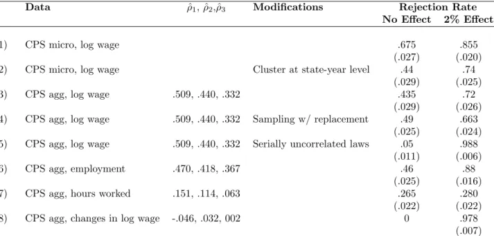
The first row of Table II presents the result of this exercise when performed in the CPS micro data, without any correction for grouped error terms. We estimate equation (1) for at least 200 independent draws of placebo laws. The control variables Xist include 4 education dummies (less

than high school, high school, some college and college or more) and a quartic in age as controls. We report the fraction of simulations in which the absolute value of the t-statistic was greater than 1.96. We find that the null of no effect is rejected a stunning 67.5 percent of the time.

One important reason for this gross over-rejection is that the estimation fails to account for correlation within state-year cells (Donald and Lang [2001], Moulton [1990]). In other words, OLS assumes that the variance-covariance matrix for the error term is diagonal while in practice it might 10_{We choose to limit the intervention date to the 1985-1995 period to ensure having enough observations prior and}

post intervention.

11

We have tried several alternative placebo interventions (such as changing the number of “affected” states or allowing for the laws to be staggered over time) and found similar effects. See Bertrand, Duflo and Mullainathan [2002] for details.

12 _{This exercise is similar in spirit to the randomly generated instruments in Bound, Jaeger and Baker [1995].}

Also, if true laws were randomly assigned, the distribution of the parameter estimates obtained using these placebo laws could be used to form a randomization inference test of the significance of the DD estimate [Rosenbaum [1996].

13

Note that we are randomizing the treatment variable while keeping the set of outcomes fixed. In general, the distribution of the test statistic induced by such randomization is not a standard normal distribution and, therefore, the exact rejection rate we should expect is not known. We directly address this issue below by turning to a more formal Monte Carlo study.

(8)

be block diagonal, with correlation of the error terms within each state-year cell. As noted earlier, while 80 of the papers we surveyed potentially suffer from this problem, only 36 correct for it. In rows 2 and 3, we account for this issue in two ways. In row 2, we allow for an arbitrary correlation of the error terms at the state-year level. We still find a very high (44 percent) rejection rate.14 In

row 3, we aggregate the data into state-year cells to construct a panel of 50 states over 21 years and then estimate the analogue of equation (1) on this data.15 Here again, we reject the null of no

effect in about 44 percent of the regressions. So correlated shocks within state-year cells explain only part of the over-rejection we observe in row 1.

In the exercise above, we randomly assigned laws over a fixed set of state outcomes. In such a case, the exact rejection rate we should expect is not known, and may be different from 5 percent even for a correctly sized test. To address this issue, we perform a Monte Carlo study where the data generating process is the state-level empirical distribution of the CPS data. Specifically, for each new simulation, we sample states with replacement from the CPS, putting probability 1/50 on each of the 50 states. Because we sample entire state vectors, this preserves the within-state autocorrelation of outcomes. In each sample, we then randomly pick half of the states to be “treated” and randomly pick a treatment year (as explained above).

The results of this Monte Carlo study (row 4) are very similar to the results obtained in the first exercise we conducted: OLS standard errors lead to reject the null hypothesis of no effect at the 5 percent significance level in 49 percent of the cases.16 To facilitate the interpretation of the

rejection rates, all the CPS results presented below are based on such Monte Carlo simulations using the state-level empirical distribution of the CPS data.

We have so far focused on Type I error. A small variant of the exercise above allows us to assess 14

Practically, this is implemented by using the “cluster” command in STATA. We also applied the correction procedure suggested in Moulton [1990]. That procedure forces a constant correlation of the error terms at the state-year level, which puts structure on the intra-cluster correlation matrices and may therefore perform better in finite samples. This is especially true when the number of clusters is small (if in fact the assumption of a constant correlation is a good approximation). The rate of rejection of the null hypothesis of no effect was not statistically different under the Moulton technique.

15 _{To aggregate, we first regress individual log weekly earnings on the individual controls (education and age)}

and form residuals. We then compute means of these residuals by state and year: ¯Yst. On this aggregated data, we estimate ¯Yst=αs+γt+β Ist+st. The results do not change if we also allow for heteroskedasticity when estimating this equation.

16

We have also run simulations where we fix the treatment year across all simulations (unpublished appendix available from the authors). The rejections rates do not vary much from year to year, and remain above 30 percent in every single year.

(9)

Type II error, or power against a specific alternative. After constructing the placebo intervention, Ist, we can replace the outcome in the CPS data by the outcome plus Ist times whichever effect

we wish to simulate. For example, we can replace log(weekly earnings) by log(weekly earnings) plus Ist×.0x to generate a true.0xlog point (approximatelyx percent) effect of the intervention.

By repeatedly estimating DD in this altered data (with new laws randomly drawn each time) and counting rejections, we can assess how often DD rejects the null of no effect under a specific alternative.17 Under the alternative of a 2 percent effect, OLS rejects the null of no effect in 66

percent of the simulations (row 4, last column).

The high rejection rate is due to serial correlation, as we document in the next rows of Table II. As we discussed earlier, an important factor is the serial correlation of the intervention variable Ist itself. In fact, if the intervention variable were not serially correlated, OLS standard errors

should be consistent. To illustrate this point, we construct a different type of intervention which eliminates the serial correlation problem. As before, we randomly select half of the states to form the treatment group. However, instead of randomly choosing one date after which all the states in the treatment group are affected by the law, we randomly select 10 dates between 1979 and 1999. The law is now defined as 1 if the observation relates to a state that belongs to the treatment group at one of these 10 dates, 0 otherwise. In other words, the intervention variable is now repeatedly turned on and off, with its value in one year telling us nothing about its value the next year. In row 5, we see that the null of no effect is now rejected in only 5 percent of the cases.

Further evidence is provided in rows 6 through 8. Here we repeat the Monte Carlo study (as in row 4) for three different variables in the CPS: employment, hours and change in log wages. We report estimates of the first, second and third order auto-correlation coefficients for each of these variables. As we see, the over-rejection problem diminishes with the serial correlation in the dependent variable. As expected, when the estimate of the first-order auto-correlation is negative (row 8), we find that OLS lead us to reject the null of no effect in less than 5 percent of the simulations.

This exercise using the CPS data illustrates the severity of the problem in a commonly used 17_{It is important to note that the “effect” we generate is uniform across states. For some practical applications,}

(10)

data set. However, one might be concerned that we are by chance detecting actual laws or other relatively discrete changes. Also, there might be other features of the CPS wage data, such as state-specific time trends, that may also give rise to over-rejection. To address this issue, we replicate our analysis in an alternative Monte Carlo study where the data generating process is an AR(1) model with normal disturbances. The data is generated so that its variance structure in terms of relative contribution of state and year fixed effects matches the empirical variance decomposition of female state wages in the CPS.18 We randomly generate a new data set and placebo laws for each

simulation. By construction, we can now be sure that there are no ambient trends and that the laws truly have no effect. In row 9, we assume that the auto-correlation parameter of the AR(1) model (ρ) equals .8. We find a rejection rate of 37 percent. In rows 10 through 14, we show that asρ goes down, the rejection rates fall. When ρ is negative (row 14), there is under-rejection.

The results in Table II demonstrate that, in the presence of positive serial correlation, con-ventional DD estimation leads to gross over-estimation of t-statistics and significance levels. In addition, the magnitudes of the estimates obtained in these false rejections do not seem out of line with what is regarded in the literature as “significant” economic impacts. The average absolute value of the estimated “significant effects” in the wage regressions is about.02, which corresponds roughly to a 2 percent effect. Nearly 60 percent of the significant estimates fall in the 1 to 2 percent range. About 30 percent fall in the 2 to 3 percent range, and the remaining 10 percent are larger than 3 percent. These magnitudes are large, considering that DD estimates are often presented as elasticities. Suppose for example that the law under study corresponds to a 5 percent increase in child-care subsidy. An increase in log earnings of .02 would correspond to an elasticity of .4. Moreover, in many DD estimates, the truly affected group is often only a fraction of the treatment group, meaning that a measured 2 percent effect on the full sample would indicate a much larger effect on the truly affected sub-sample.

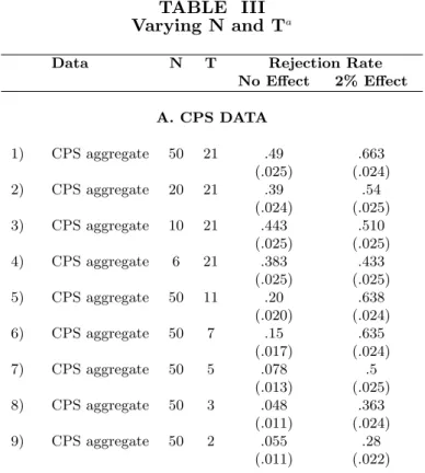
The stylized exercise above focused on data with 50 states and 21 time periods. Many DD papers use fewer states (or treated and control units), either because of data limitations or because of a desire to focus only on comparable controls. For similar reasons, several DD papers use fewer 18 _{We choose an AR(1) process to illustrate the problems caused by auto-correlation in the context of a simple}

(11)

time periods. In Table III, we examine how the rejection rate varies with these two important parameters. We rely on the Monte Carlo studies described above (state-level empirical distribution of the CPS data and AR(1) model with normal disturbances) to analyze these effects. We also report rejection rates when we add a 2 percent treatment effect to the data.

The data sets used by many researchers have fewer than 50 groups. Rows 1-4 and 10-13 show that varying the number of states does not change the extent of the over-rejection. Rows 5-9 and 14-17 vary the number of years. As expected, over-rejection falls as the time span gets shorter, but it does so at a rather slow rate. For example, even with only 7 years of data, the rejection rate is 15 percent in the CPS-based simulations. Conditional on using more than 2 periods, around 60 percent of the DD papers in our survey use at least 7 periods. With 5 years of data, the rejection rate varies between 8 percent (CPS) and 17 percent (AR(1), ρ = 8). When T=50, the rejection rate rises to nearly 50 percent in the simulations using an AR(1) model withρ=.8.

IV. Solutions

In this section, we evaluate the performance of alternative estimators that have been proposed in the literature to deal with serial correlation. To do so, we use placebo interventions in the two Monte Carlo studies described above. We also evaluate the power of each estimator against the specific alternative of a 2 percent effect (we addIst∗0.02 to the data). The choice of 2 percent as

the alternative is admittedly somewhat arbitrary, but our conclusions on the relative power of each estimator do not dependent on this specific value.19

IV.A. Parametric Methods

A first possible solution to the serial correlation problem would be to specify an auto-correlation structure for the error term, estimate its parameters, and use these parameters to compute standard errors. This is the method that was followed in 4 of the 5 surveyed DD papers that attempted

19

We report the power against the alternative of 2 percent because 2 percent appears as a “reasonable” size effect. Moreover, in simulated data with an AR(1) process withρ=0.8, the rejection rate when using thetrue variance-covariance matrix is 32.5 percent when there is a 2 percent effect, which is large enough to be very different from the 5 percent rejection rate obtained under the null of no effect.

(12)

to deal with serial correlation. We implement several variations of this basic correction method in Table IV.

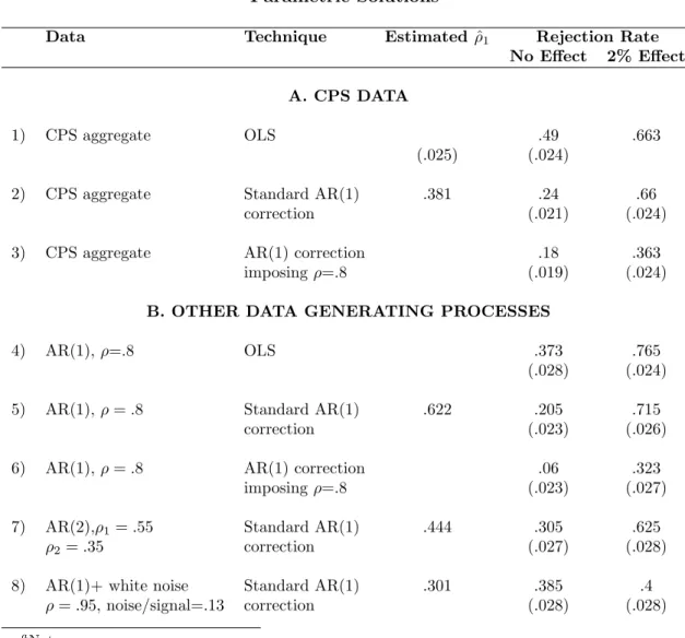
Row 2 performs the simplest of these parametric corrections, wherein an AR(1) process is estimated in the data, without correction for small sample bias in the estimation of the AR(1) parameter. We first estimate the first order auto-correlation coefficient of the residual by regressing the residual on its lag, and then use this estimated coefficient to form an estimate of the block-diagonal variance-covariance matrix of the residual. This technique does little to solve the serial correlation problem: the rejection rate stays high at 24 percent. The results are the same whether or not we assume that each state has its own auto-correlation parameter. The failure of this correction method is in part due to the downward bias in the estimator of the auto-correlation coefficient. As is already well understood, with short time-series, the OLS estimation of the auto-correlation parameter is biased downwards. In the CPS data, OLS estimates a first-order auto-correlation coefficient of only 0.4. Similarly, in the AR(1) model where we know that the auto-correlation parameter is.8, a ˆρ of.62 is estimated (row 5). However, if we impose a first-order autocorrelation of .8 in the CPS data (row 3), the rejection rate only goes down to 16 percent, a very partial improvement.

Another likely problem with the parametric correction may be that we have not correctly specified the auto-correlation process. As noted earlier, an AR(1) does not fit the correlogram of wages in the CPS. In rows 7 and 8, we use new Monte Carlo simulations to assess the effect of such a mis-specification of the autocorrelation process. In row 7, we generate data according to an AR(2) process withρ1 =.55 andρ2=.35. These parameters were chosen because they match well

the estimated first, second and third auto-correlation parameters in the wage data when we apply the formulas to correct for small sample bias given in Solon [1984]. We then correct the standard error assuming that the error term follows an AR(1) process. The rejection rate rises significantly with this mis-specification of the auto-correlation structure (30.5 percent).

In row 8, we use a data generating process that provides an even better match of the time-series properties of the CPS data: the sum of an AR(1) (with auto-correlation parameter 0.95) plus white noise (the variance of the white noise is 13 percent of the total variance of the residual). When trying to correct the auto-correlation in this data by fitting an AR(1), we reject the null of no effect

(13)

in about 39 percent of the cases.

The parametric corrections we have explored do not appear to provide an easy solution for the applied researcher.20 _{Any mis-specification of the data generating process results in inconsistent}

standard errors and, at least without much deeper exploration into specification tests, it is difficult to find the true data generating process.21

We next investigate alternative techniques that make little or no specific assumption about the structure of the error term. We start by examining a simulation-based technique. We then examine three other techniques that can be more readily implemented using standard statistical packages.

IV.B. Block Bootstrap

Block bootstrap [Efron and Tibshirani, 1994] is a variant of bootstrap which maintains the auto-correlation structure by keeping all the observations that belong to the same group (e.g., state) together. In practice, we bootstrap the t-statistic as follows. For each placebo intervention, we compute the absolute t-statistic t=abs( ˆβ/SE( ˆβ)), using the OLS estimate of β and its standard error. We then construct a bootstrap sample by drawing with replacement 50 matrices ( ¯Ys,Vs),

where ¯Ys is the entire time series of observations for states, andVsis the matrix of state dummies,

time dummies, and treatment dummy for state s. We then run OLS on this sample, obtain an estimate ˆβr and construct the absolute t-statistictr= abs( ˆβr−

ˆ

β)

SE( ˆβr) . The sampling distribution oftr is

random and changing asN (the number of states) grows. The difference between this distribution and the sampling distribution of t becomes small as N goes to infinity, even in the presence of arbitrary auto-correlation within states and heteroskedasticity. We draw a large number (200) of bootstrap samples, and reject the hypothesis that β = 0 at a 95 percent confidence level if 95 percent of thetr are smaller thant. The results of the block bootstrap estimation are reported in

Table V.

This correction method presents a major improvement over the parametric techniques discussed 20

We do not explore in this paper IV/GMM estimation techniques. There is however a large literature on GMM estimation of dynamic panel data models that could potentially be applied here.

21

For example, when we use the two “reasonable” processes described above in the CPS data or in a Monte Carlo study based on the empirical distribution of the CPS data, the rejection rates remained high.

(14)

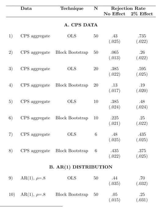
before. When N equals 50, the rejection rate of the null of no effect is 6.5 percent in data drawn from the CPS and 5 percent in data drawn from an AR(1) model. When there is a 2 percent effect, the null of no effect is rejected in 26 percent of the cases in the CPS data and in 25 percent of the cases in the AR(1) data. However, the method performs less well when the number of states declines. The rejection rate is 13 percent with 20 states and 23 percent with 10 states. The power of this test also declines quite fast. With 20 states, the null of no effect is rejected in only 19 percent of the cases when there is a 2 percent effect.

While block bootstrap provides a reliable solution to the serial correlation problem when the number of groups is large enough, this technique is rarely used in practice by applied researchers, perhaps because it is not immediate to implement.22 We therefore now turn to three simpler

correction methods.

IV.C. Ignoring Time Series Information

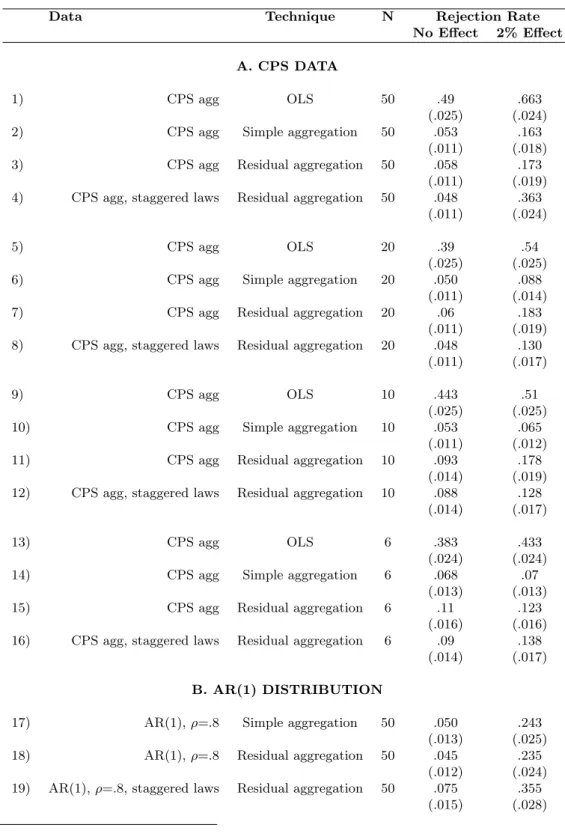
The first simpler method we investigate is to ignore the time series information when computing standard errors. To do this, one could simply average the data before and after the law and run equation (1) on this averaged outcome variable in a panel of length 2. The results of this exercise are reported in Table VI. The rejection rate when N equals 50 is now 5.3 percent (row 2).

Taken literally, however, this solution will work only for laws that are passed at the same time for all the treated states. If laws are passed at different times, “before” and “after” are no longer the same for each treated state and not even defined for the control states. One can however slightly modify the technique in the following way. First, one can regress Yst on state fixed effects, year

dummies, and any relevant covariates. One can then divide the residuals of the treatment states onlyinto two groups: residuals from years before the laws, and residuals from years after the laws. The estimate of the laws’ effect and its standard error can then be obtained from an OLS regression in this two-period panel. This procedure does as well as the simple aggregation (row 3 vs. row 2) for laws that are all passed at the same time. It also does well when the laws are staggered over

22

Implementing block bootstrap does require a limited amount of programming. The codes generated for this study are available upon request.

(15)

time (row 4).23

When the number of states is small, the t-statistic needs to be adjusted to take into account the smaller number of observations (see Donald and Lang [2001] for a discussion of inference in small-sample aggregated data set). When we do that, simple aggregation continues to perform well, even for quite small numbers of states. Residual aggregation performs a little worst, but the over-rejection remains relatively small. For example, for 10 states, the rejection rate is 5.3 percent under the simple aggregation method (row 10) and about 9 percent under the residual aggregation method (row 11).

The downside of these procedures (both raw and residual aggregation) is that their power is quite low and diminishes fast with sample size. In the CPS simulations with a 2 percent effect, simple aggregation rejects the null only 16 percent of the time with 50 states (row 2), 8.8 percent of time with 20 states (row 6), and 6.5 percent of the time with 10 states (row 10).

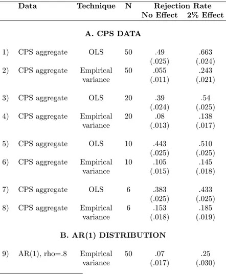
IV.D. Empirical Variance-Covariance Matrix

As we have seen in Section IV.A, parametric corrections seem to fail in practice. However, the parametric techniques discussed above did not make use of the fact that we have a large number of states that can be used to estimate the auto-correlation process in a more flexible fashion. Specifically, suppose that the auto-correlation process is the same across all states and that there is no cross-sectional heteroskedasticity. In this case, if the data is sorted by states and (by decreasing order of) years, the variance-covariance matrix of the error term is block diagonal, with 50 identical blocks of sizeT by T (where T is the number of time periods). Each of these blocks is symmetric, and the element (i, i+j) is the correlation betweeni andi−j. We can therefore use the variation

across the 50 states to estimate each element of this matrix, and use this estimated matrix to compute standard errors. Under the assumption that there is no heteroskedasticity, this method will produce consistent estimates of the standard error asN (the number of groups) goes to infinity (Kiefer [1980]).

23_{To generate staggered laws, we randomly choose half of the states to form the treatment group and randomly}

(16)

Table VII investigates how well this technique performs in practice in the CPS and AR(1) Monte Carlo studies. The method performs well when the number of states is large (N=50). The rejection rate we obtain in this case is 5.5 percent in the CPS (row 2) and 7 percent in the Monte Carlo simulations (row 9). Its power when N=50 is comparable to the power of the block bootstrap method. In the Monte Carlo study based on the empirical distribution of the CPS, we reject the null of no effect in 24 percent of the simulations when there is a 2 percent effect.

However, as Table VII also indicates, this method performs more poorly for small sample sizes. As the number of states drop, the rejection rate of the null of no effect increases. For N=10, this correction method leads us to reject the null of no effect in 8 percent of the cases; for N=6, the rejection rate is 15 percent.

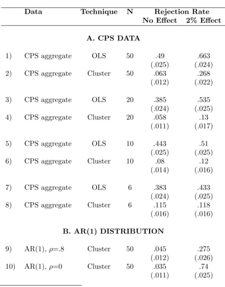
IV.E. Arbitrary Variance-Covariance Matrix

One obvious limitation of the empirical variance-covariance matrix method discussed above is that it is only consistent under the assumption of cross-sectional homoskedasticity, an assumption that is likely to be violated in practice for many data sets. However, this method can be generalized to an estimator of the variance-covariance matrix which is consistent in the presence of any cor-relation pattern within states over time. Of course, we cannot consistently estimate each element of the variance-covariance matrix in this case, but we can use a generalized White-like formula to compute the standard errors (White [1984], Arellano [1987] and Kezdi [2002]).24 This estimator

for the variance-covariance matrix is given by:

W = (V0V)−1



 N X

j=1

u0_juj 

(V 0

V)−1

where N is the total number of states,V is matrix of independent variables (year dummies, state dummies and treatment dummy) anduj is defined for each state to be:

uj = T X

t=1

ejtvjt

24 _{This is analogous to applying the Newey-West correction (Newey and West [1987]) in the panel context where}

(17)

whereejtis the estimated residual for stateiat timetandvjt is a row vector of dependent variables

(including the constant).25 This estimator of the variance-covariance matrix is consistent for fixed

panel length as the number of states tends to infinity [Kezdi 2002].26

In Table VIII, we investigate how well this estimation procedure performs in practice in finite samples. Despite its generality, the arbitrary variance-covariance matrix does quite well. The rejection rate in data drawn CPS is 6.3 percent when N=50 (row 2). With respect to power, we saw in Tables II and IV that with the correct covariance matrix, the rejection rate in the case of a 2 percent effect was 78 percent in a Monte Carlo simulation with no auto-correlation and 32 percent in AR(1) data with ρ = .8. The arbitrary variance-covariance matrix comes near these upper-bounds, achieving rejection rates of 74 percent (row 10) and 27.5 percent (row 9) respectively. Again, however, rejection rates increase significantly above 5 percent when the number of states declines: 11.5 percent with 6 states (row 8), 8 percent with 10 states (row 6). The extent of the over-rejection in small samples is comparable to that obtained for the empirical variance-covariance matrix correction method, less extreme than with block bootstrap, but higher than with the time series aggregation.

IV.F. Summary

Based on Monte Carlo simulations, this section has reviewed the performance of several stan-dard correction methods for serial correlation. The results we obtain are in accord with the previous literature. First, “naive” parametric corrections, which do not take into account the bias in the estimation of the auto-correlation parameters in short time series, perform poorly (Nickell [1981]). Furthermore, the time series lengths typical to DD applications are generally too short to reli-ably estimate more flexible data generating processes and mis-specification of the process leads to inconsistent standard errors (Greene [2002]).

Second, the arbitrary and empirical variance-covariance matrix corrections perform well in large 25

This is implemented in a straightforward way by using the cluster command in STATA and choosing entire states (and not only state-year cells) as clusters.

26

Note that the resulting variance-covariance matrix is of rankT N−N. The standard error of the coefficient of the state dummies is not identified in this model. However the other terms of the variance-covariance matrix are identified and consistently estimated asN goes to infinity.

(18)

samples, but not as well when the number of groups becomes small. The small sample bias in the White standard errors were already noted in MacKinnon and White [1985], who perform Monte Carlo simulations of this estimator, as well as of alternative estimators with better finite sample properties. Also, Bell and McAffrey [2002] compute the small sample bias of the White standard errors. They show that this bias is larger for variables that are constant or nearly constant within cluster (which is the case of the treatment variables in the DD model). Kezdi [2002] performs Monte Carlo simulations to evaluate the small sample properties of the Huber-White and the empirical variance-covariance estimators of the standard errors in a fixed effect model with serial correlation. Both estimators perform well in finite sample when N equals 50, but are biased when N equals 10. Finally, aggregating the time series information performs well even for small number of states, which reflects the fact that the significance threshold can be adjusted for the small effective sample size (Donald and Lang [2001]). However, these aggregation techniques have relatively low power.

V. Conclusion

Our study suggests that, because of serial correlation, conventional DD standard errors may grossly understate the standard deviation of the estimated treatment effects, leading to serious over-estimation of t-statistics and significance levels. Since a large fraction of the published DD papers we surveyed report t-statistics around 2, our results suggest that some of these findings may not be as significant as previously thought if the outcome variables under study are serially correlated. In other words, it is possible that too many false rejections of the null hypothesis of no effect have taken place.

We have investigated how several standard estimation methods help deal with the serial correla-tion problem in the DD context. We show that block bootstrap can be used to compute consistent standard errors when the number of groups is sufficiently large. Moreover, we show that a few techniques that are readily available in standard econometrics packages also provide viable solu-tions for the applied researcher. Collapsing the data into pre- and post- periods produce consistent standard errors, even when the number of states is small (though the power of this test declines fast). Allowing for an arbitrary auto-correlation process when computing the standard errors is

(19)

also a viable solution when the number of groups is sufficiently large.

We hope that our study provides some motivation for the practitioners that estimate DD models to more carefully examine residuals as well as perform simple tests of serial correlation. Because computing standard errors that are robust to serial correlation appears relatively easy to implement in most cases, it should become standard practice in applied work. We also hope that our study will contribute in generating further work on alternative estimation methods for DD models (such as GLS estimation or GMM estimation of dynamic panel data models) that could be more efficient in the presence of serial correlation.

(20)

UNIVERSITY OF CHICAGO GRADUATE SCHOOL OF BUSINESS, NATIONAL BUREAU OF ECONOMIC RESEARCH AND CENTER FOR ECONOMIC POLICY RESEARCH

MASSACHUSSETS INSTITUTE OF TECHNOLOGY, NATIONAL BUREAU OF ECONOMIC RESEARCH AND CENTER FOR ECONOMIC POLICY RESEARCH

MASSACHUSSETS INSTITUTE OF TECHNOLOGY AND NATIONAL BUREAU OF ECO-NOMIC RESEARCH

(21)

References

Abadie, Alberto, “Semiparametric Difference-in-Differences Estimators,” Working Paper, Kennedy School of Government, Harvard University, 2000.

Arellano, Manuel, “Computing Robust Standard Errors for Within-Groups Estimators,” Oxford Bulletin of Economics and Statistics, XLIX (1987), 431-434.

Athey, Susan, and Guido Imbens, “Identification and Inference in Nonlinear Difference-in-Differences Models,” National Bureau of Economic Research Technical Working Paper No. T0280, 2002.

Bell, Robert, and Daniel McCaffrey, “Bias Reduction for Standard Errors for Linear Regressions with Multi-Stage Samples,” RAND Working Paper, 2002.

Bertrand, Marianne, Esther Duflo, and Sendhil Mullainathan, “How Much Should We Trust Differences-in-Differences Estimates?” National Bureau of Economic Research Working Paper No. 8841, 2002.

Besley, Timothy, and Anne Case, “Unnatural Experiments? Estimating the Incidence of Endoge-nous Policies,” Economic Journal, CDLXVII (2000), F672-F694.

Blanchard, Olivier, and Lawrence Katz, “Regional Evolutions,” Brookings Papers on Economic Activity, I (1992), 1-75.

Blanchard, Olivier, and Lawrence Katz, “What We Know and Do Not Know about the Natural Rate of Unemployment,”Journal of Economic Perspectives, XI (1997), 51-72.

Blundell, Richard, and Thomas MaCurdy, “Labor Supply,” inHandbook of Labor Economics, Orley Ashenfelter and David Card, eds. (Amsterdam: North-Holland, 1999).

Bound, John, David Jaeger, and Regina Baker, “Problems with Instrumental Variables Estimation When the Correlation Between the Instruments and the Endogeneous Explanatory Variable is Weak,”Journal of the American Statistical Association, XC (1995), 443-450.

Donald, Stephen, and Kevin Lang, “Inferences with Difference in Differences and Other Panel Data,” Working Paper, Boston University, 2001.

Efron, Bradley, and Robert Tibshirani, An Introduction to the Bootstrap, Monograph in Applied Statistics and Probability, No. 57 (New York, NY: Chapman and Hall, 1994).

(22)

Results,”Journal of the American Statistical Association, LXXIX (1984), 97-106.

Greene, William H.,Econometric Analysis (New York, NY: Prentice Hall, 2002).

Heckman, James, “Causal Parameters and Policy Analysis in Economics: A Twentieth Century Retrospective,”The Quarterly Journal of Economics, CXV (2000), 45-97.

Kezdi, Gabor, “Robust Standard Error Estimation in Fixed-Effects Panel Models,” Working Paper, University of Michigan, 2002.

Kiefer, N.M., “Estimation of Fixed Effect Models for Time Series of Cross Section with Arbitrary Intertemporal Covariance,”Journal of Econometrics, XIV (1980), 195-202.

MacKinnon, James G., and Halbert White, “Some Heteroskedasticity-Consistent Covariance Ma-trix Estimators with Improved Finite Sample Properties,” Journal of Econometrics, XXIX (1985), 305-325.

Meyer, Bruce, “Natural and Quasi-Natural Experiments in Economics,” Journal of Business and Economic Statistics, XII (1995), 151-162.

Moulton, Brent R., “An Illustration of a Pitfall in Estimating the Effects of Aggregate Variables in Micro Units,” Review of Economics and Statistics, LXXII (1990), 334-338.

Newey, Whitney, and K. D. West, “A Simple, Positive Semi-definite, Heteroskedasticity and Auto-correlation Consistent-Covariance Matrix,”Econometrica, LV (1987), 703-708.

Nickell, Stephen, “Biases in Dynamic Models with Fixed Effects,” Econometrica, XLIX (1981), 1417-1426.

Rosenbaum, Paul, “Observational Studies and Nonrandomized Experiments,” in Handbook of Statistics, S. Ghosh and C.R. Rao, eds. (New York, NY: Elsevier, 1996).

Solon, Gary, “Estimating Auto-correlations in Fixed-Effects Models,” National Bureau of Economic Research Technical Working Paper No. 32, 1984.

White, Halbert, Asymptotic Theory for Econometricians(San Diego, CA: Academic Press, 1984).

Wooldridge, Jeffrey M.,Econometric Analysis of Cross Section and Panel Data (Cambridge, MA: MIT Press, 2002).

(23)

Wooldridge, Jeffrey M., “Cluster-Sample Methods in Applied Econometrics,” American Economic Review, XCIII (2003), 133-138.

(24)

TABLE I Survey of DD Papersa

Number of DD papers 92

Number with more than 2 periods of data 69 Number which collapse data into before-after 4

Number with potential serial correlation problem 65

Number with some serial correlation correction 5

GLS 4

Arbitrary variance-covariance matrix 1

Distribution of time span for papers with more than 2 periods Average 16.5

Percentile Value

1% 3

5% 3

10% 4

25% 5.75

50% 11

75% 21.5

90% 36

95% 51

99% 83

Most commonly used dependent variables Number

Employment 18 Wages 13 Health/medical expenditure 8

Unemployment 6 Fertility/teen motherhood 4 Insurance 4 Poverty 3 Consumption/savings 3

Informal techniques used to assess endogeneity Number

Graph dynamics of effect 15

See if effect is persistent 2

DDD 11

Include time trend specific to treated states 7

Look for effect prior to intervention 3

Include lagged dependent variable 3

Number with potential clustering problem 80

Number which deal with it 36

a_{Notes: Data comes from a survey of all articles in six journals between 1990 and 2000:}_the

American Economic Review;the Industrial Labor Relations Review;the Journal of Labor Economics;

the Journal of Political Economy;the Journal of Public Economics; andthe Quarterly Journal of Economics. We define an article as “Difference-in-Difference” if it: (1) examines the effect of a specific intervention and (2) uses units unaffected by the intervention as a control group.

(25)

TABLE II

DD Rejection Rates for Placebo Lawsa

A. CPS DATA

Data ρˆ1, ˆρ2, ˆρ3 Modifications Rejection Rate

No Effect 2% Effect

1) CPS micro, log wage .675 .855

(.027) (.020) 2) CPS micro, log wage Cluster at state-year level .44 .74

(.029) (.025)

3) CPS agg, log wage .509, .440, .332 .435 .72

(.029) (.026) 4) CPS agg, log wage .509, .440, .332 Sampling w/ replacement .49 .663

(.025) (.024) 5) CPS agg, log wage .509, .440, .332 Serially uncorrelated laws .05 .988

(.011) (.006)

6) CPS agg, employment .470, .418, .367 .46 .88

(.025) (.016)

7) CPS agg, hours worked .151, .114, .063 .265 .280

(.022) (.022) 8) CPS agg, changes in log wage -.046, .032, 002 0 .978

(.007)

B. MONTE CARLO SIMULATIONS WITH SAMPLING FROM AR(1) DISTRIBUTION

Data ρ Modifications Rejection Rate

No Effect 2% Effect

9) AR(1) .8 .373 .725

(.028) (.026)

10) AR(1) 0 .053 .783

(.013) (.024)

11) AR(1) .2 .123 .738

(.019) (.025)

12) AR(1) .4 .19 .713

(.023) (.026)

13) AR(1) .6 .333 .700

(.027) (.026)

14) AR(1) −.4 .008 .7

(.005) (.026)

a_Notes:

a. Unless mentioned otherwise under ”Modifications,” reported in the last two columns are the OLS rejection rates of the null hypothesis of no effect (at the 5 percent significance level) on the intervention variable for randomly generated placebo interventions as described in text. The data used in the last column was altered to simulate a true 2 percent effect of the intervention. The number of simulations for each cell is at least 200 and typically 400.

b. CPS data are data for women between 25 and 50 in the fourth interview month of the Merged Outgoing Rotation Group for the years 1979 to 1999. In rows 3 to 8 of Panel A, data are aggregated to state-year level cells after controlling for demographic variables (4 education dummies and a quartic in age). For each simulation in rows 1 through 3, we use the observed CPS data. For each simulation in rows 4 through 8, the data generating process is the state-level empirical distribution of the CPS data that puts a probability of 1/50 on the different states’ outcomes (see text for details). For each simulation in Panel B, the data generating process is an AR(1) model with normal disturbances chosen to match the CPS state female wage variances (see text for details). ˆρirefer to the estimated auto-correlation parameter of lagi. ρrefers to the auto-correlation parameter in the AR(1) model. c. All regressions include, in addition to the intervention variable, state and year fixed effects. The

(26)

TABLE III Varying N and Ta

Data N T Rejection Rate No Effect 2% Effect A. CPS DATA

1) CPS aggregate 50 21 .49 .663

(.025) (.024)

2) CPS aggregate 20 21 .39 .54

(.024) (.025)

3) CPS aggregate 10 21 .443 .510

(.025) (.025)

4) CPS aggregate 6 21 .383 .433

(.025) (.025)

5) CPS aggregate 50 11 .20 .638

(.020) (.024)

(.017) (.024)

(.013) (.025)

8) CPS aggregate 50 3 .048 .363

(.011) (.024)

(.011) (.022) B. MONTE CARLO SIMULATIONS

WITH SAMPLING FROM AR(1) DISTRIBUTION

10) AR(1),ρ=.8 50 21 .35 .638

(.028) (.028)

11) AR(1),ρ=.8 20 21 .35 .538

(.028) (.029)

12) AR(1),ρ=.8 10 21 .3975 .505

(.028) (.029)

13) AR(1),ρ=.8 6 21 .393 .5

(.028) (.029)

14) AR(1),ρ=.8 50 11 .335 .588

(.027) (.028)

15) AR(1),ρ=.8 50 5 .175 .5525

(.022) (.029)

16) AR(1),ρ=.8 50 3 .09 .435

(.017) (.029)

17) AR(1),ρ=.8 50 50 .4975 .855

(.029) (.020) a

Notes:

a. Reported in the last two columns are the OLS rejection rates of the null hypothesis of no effect (at the 5 percent significance level) on the intervention variable for randomly generated placebo interventions as described in text. The data used in the last column was altered to simulate a true 2 percent effect of the intervention. The number of simulations for each cell is typically 400 and at least 200. b. CPS data are data for women between 25 and 50 in the fourth interview month of the Merged Outgoing

Rotation Group for the years 1979 to 1999. The dependent variable is log weekly earnings. Data are aggregated to state-year level cells after controlling for the demographic variables (4 education dummies and a quartic in age). For each simulation in Panel A, the data generating process is the state-level empirical distribution of the CPS data that puts a probability of 1/50 on the different states’ outcomes (see text for details). For each simulation in Panel B, the data generating process is an AR(1) model with normal disturbances chosen to match the CPS state female wage variances (see text for details). ρrefers to the auto-correlation parameter in the AR(1) data generating process. c. All regressions also include, in addition to the intervention variable, state and year fixed effects. d. Standard errors are in parenthesis and are computed using the number of simulations.

(27)

TABLE IV Parametric Solutionsa

Data Technique Estimated ρˆ1 Rejection Rate

No Effect 2% Effect

A. CPS DATA

1) CPS aggregate OLS .49 .663

(.025) (.024)

2) CPS aggregate Standard AR(1) .381 .24 .66

correction (.021) (.024)

3) CPS aggregate AR(1) correction .18 .363

imposingρ=.8 (.019) (.024)

B. OTHER DATA GENERATING PROCESSES

4) AR(1),ρ=.8 OLS .373 .765

(.028) (.024) 5) AR(1),ρ=.8 Standard AR(1) .622 .205 .715

correction (.023) (.026)

6) AR(1),ρ=.8 AR(1) correction .06 .323

imposingρ=.8 (.023) (.027)

7) AR(2),ρ1=.55 Standard AR(1) .444 .305 .625

ρ2=.35 correction (.027) (.028)

8) AR(1)+ white noise Standard AR(1) .301 .385 .4

ρ=.95, noise/signal=.13 correction (.028) (.028)

a Notes:

a. Reported in the last two columns are the rejection rates of the null hypothesis of no effect (at the 5 percent significance level) on the intervention variable for randomly generated placebo interventions as described in text. The data used in the last column was altered to simulate a true 2 percent effect of the intervention. The number of simulations for each cell is typically 400 and at least 200.

b. CPS data are data for women between 25 and 50 in the fourth interview month of the Merged Outgoing Rotation Group for the years 1979 to 1999. The dependent variable is log weekly earnings. Data are aggregated to state-year level cells, after controlling for the demographic variables (4 education dummies and a quartic in age). For each simulation in Panel A, the data generating process is the state-level empirical distribution of the CPS data that puts a probability of 1/50 on the different states’ outcomes (see text for details). For each simulation in Panel B, the distributions from which the data are drawn are chosen to match the CPS state female wage variances (see text for details). “AR(1)+ white noise” is the sum of an AR(1) plus an i.i.d. process, where the auto-correlation for the AR(1) component is given byρand the relative variance of the components is given by the noise to signal ratio. c. All regressions include, in addition to the intervention variable, state and year fixed effects. d. Standard errors are in parenthesis and are computed using the number of simulations. e. The AR(k) corrections are implemented in stata using the “xtgls” command.

(28)

TABLE V Block Bootstrapa

Data Technique N Rejection Rate

No Effect 2% Effect

A. CPS DATA

1) CPS aggregate OLS 50 .43 .735

(.025) (.022) 2) CPS aggregate Block Bootstrap 50 .065 .26

(.013) (.022)

(.017) (.020)

(.021) (.022)

(.022) (.025)

B. AR(1) DISTRIBUTION

9) AR(1),ρ=.8 OLS 50 .44 .70

(.035) (.032) 10) AR(1),ρ=.8 Block Bootstrap 50 .05 .25

(.015) (.031)

a Notes:

a. Reported in the last two columns are the rejection rates of the null hypothesis of no effect (at the 5 percent significance level) on the intervention variable for randomly generated placebo interventions as described in text. The data used in the last column was altered to simulate a true 2 percent effect of the intervention. The number of simulations for each cell is typically 400 and at least 200. The bootstraps involve 400 repetitions.

b. CPS data are data for women between 25 and 50 in the fourth interview month of the Merged Outgoing Rotation Group for the years 1979 to 1999. The dependent variable is log weekly earnings. Data are aggregated to state-year level cells after controlling for the demographic variables (4 education dummies and a quartic in age). For each simulation, we draw each state’s vector from this data with replacement. See text for details. The AR(1) distribution is chosen to match the CPS state female wage variances (see text for details).

c. All CPS regressions also include, in addition to the intervention variable, state and year fixed effects.

(29)

TABLE VI

Ignoring Time Series Dataa

Data Technique N Rejection Rate No Effect 2% Effect A. CPS DATA

1) CPS agg OLS 50 .49 .663

(.025) (.024)

2) CPS agg Simple aggregation 50 .053 .163

(.011) (.018)

3) CPS agg Residual aggregation 50 .058 .173

(.011) (.019) 4) CPS agg, staggered laws Residual aggregation 50 .048 .363

(.011) (.024)

5) CPS agg OLS 20 .39 .54

(.025) (.025)

(.011) (.014)

(.011) (.017)

9) CPS agg OLS 10 .443 .51

(.025) (.025)

(.011) (.012)

(.014) (.017)

13) CPS agg OLS 6 .383 .433

(.024) (.024)

(.013) (.013)

(.014) (.017) B. AR(1) DISTRIBUTION

17) AR(1),ρ=.8 Simple aggregation 50 .050 .243

(.013) (.025)

18) AR(1),ρ=.8 Residual aggregation 50 .045 .235

(.012) (.024) 19) AR(1),ρ=.8, staggered laws Residual aggregation 50 .075 .355

(.015) (.028) a_Notes:

b. CPS data are data for women between 25 and 50 in the fourth interview month of the Merged Outgoing Rotation Group for the years 1979 to 1999. The dependent variable is log weekly earnings. Data are aggregated to state-year level cells after controlling for demographic variables (4 education dummies and a quartic in age). For each simulation, we draw each state’s vector from this data with replacement. See text for details. The AR(1) distribution is chosen to match the CPS state female wage variances (see text for details).

(30)

TABLE VII

Empirical Variance-Covariance Matrixa

No Effect 2% Effect

A. CPS DATA

1) CPS aggregate OLS 50 .49 .663 (.025) (.024) 2) CPS aggregate Empirical 50 .055 .243

variance (.011) (.021) 3) CPS aggregate OLS 20 .39 .54

(.024) (.025) 4) CPS aggregate Empirical 20 .08 .138

variance (.018) (.019)

9) AR(1), rho=.8 Empirical 50 .07 .25 variance (.017) (.030)

a_Notes:

b. CPS data are data for women between 25 and 50 in the fourth interview month of the Merged Outgoing Rotation Group for the years 1979 to 1999. The dependent variable is log weekly earnings. Data are aggregated to state-year level cells after controlling for demographic variables (4 education dummies and a quartic age). For each simulation, we draw each state’s vector from this data with replacement. See text for details. The AR(1) distribution is chosen to match the CPS state female wage variances (see text for details).

c. All regressions include, in addition to the intervention variable, state and year fixed effects. d. Standard errors are in parenthesis and are computed using the number of simulations.

(31)

TABLE VIII

Arbitrary Variance-Covariance Matrixa

No Effect 2% Effect

A. CPS DATA

1) CPS aggregate OLS 50 .49 .663 (.025) (.024) 2) CPS aggregate Cluster 50 .063 .268

(.012) (.022) 3) CPS aggregate OLS 20 .385 .535

(.024) (.025) 4) CPS aggregate Cluster 20 .058 .13

(.016) (.016)

9) AR(1), ρ=.8 Cluster 50 .045 .275 (.012) (.026) 10) AR(1), ρ=0 Cluster 50 .035 .74

(.011) (.025)

a_Notes:

a. Reported in the last two columns are the rejection rates of the null hypothesis of no effect (at the 5 percent significance level) on the intervention variable for randomly generated placebo interventions as described in text. The data used in the last column was altered to simulate a true 2 percent effect of the intervention. The number of simulations for each cell is typically 400 and at least 200. b. CPS data are data for women between 25 and 50 in the fourth interview month of the Merged Outgoing

Rotation Group for the years 1979 to 1999. The dependent variable is log weekly earnings. Data are aggregated to state-year level cells after controlling for the demographic variables (4 education dummies and a quartic in age). For each simulation, we draw each state’s vector from this data with replacement. See text for details. The AR(1) distribution is chosen to match the CPS state female wage variances (see text for details).

c. All regressions also include, in addition to the intervention variable, state and year fixed effects. d. Standard errors are in parenthesis and are computed using the number of simulations.

(32)

UNPUBLISHED APPENDIX

TABLE IX Results by Year of Lawa

Data Technique Year Rejection Rate

No Effect 2% Effect

CPS aggregate OLS 1985 .453 .658 (.025) (.024) CPS aggregate OLS 1986 .42 .688

(.025) (.023) CPS aggregate OLS 1987 .5 .638

(.024) (.024)

a_Notes:

a. Reported in the last two columns are the rejection rates of the null hypothesis of no effect (at the 5 percent significance level) on the intervention variable for randomly generated placebo interventions as described in text. The data used in the last column was altered to simulate a true 2 percent effect of the intervention. The number of simulations for each cell is typically 400 and at least 200. Each row represents a different fixed year for the law.

b. CPS data are data for women between 25 and 50 in the fourth interview month of the Merged Outgoing Rotation Group for the years 1979 to 1999. The dependent variable is log weekly earnings. Data are aggregated to state-year level cells after controlling for the demographic variables (4 education dummies and a quartic in age). For each simulation, we draw each state’s vector from this data with replacement. See text for details.

c. All regressions also include, in addition to the intervention variable, state and year fixed effects. d. Standard errors are in parenthesis and are computed using the number of simulations.