Sharif University of Technology
Scientia IranicaTransactions E: Industrial Engineering www.scientiairanica.com
A fuzzy dynamic multi-objective multi-item model by
considering customer satisfaction in a supply chain
S. Fazli Besheli
a;, R. Nemati Keshteli
b, S. Emami
cand S.M. Rasouli
aa. Department of Industrial Engineering, Mazandaran Institute of Technology, Babol, Mazandaran, P.O. Box 744, Iran. b. Faculty of Engineering, University of Guilan, East Guilan, Rasht, P.O. Box 1841, Iran.
c. Department of Industrial Engineering, Babol Noshirvani University of Technology, Babol, Mazandaran, P.O. Box 484, Iran. Received 2 February 2016; received in revised form 20 July 2016; accepted 1 October 2016
KEYWORDS Supply chain optimization; Transportation risk; Customer satisfaction; Quality.
Abstract. Customer satisfaction is an important issue in competitive strategic manage-ment of companies. Logistical and cross-functional drivers of supply chain have an impor-tant role in managing customer satisfaction. Customer satisfaction depends on quality, cost, and delivery. In this paper, a fuzzy mixed integer nonlinear programming model is proposed for a multi-item multi-period problem in a multi-level supply chain. Minimization of costs, manufacturing and transportation time, transportation risks, maximization of quality by minimizing the number of defective products, and maximization of customers' service levels are considered to be objective functions of the model. Furthermore, it is assumed that the demand rates are fuzzy values. An exact "-constraint approach is used to solve the problem. The problem is computationally intractable. Therefore, the Non-dominant Sorting Genetic Algorithm (NSGA-II) is developed to solve it. The Taguchi method is utilized to tune the NSGA-II parameters. Finally, some numerical examples are generated and solved to evaluate the performance of the proposed model and solving methods.
© 2017 Sharif University of Technology. All rights reserved.
1. Introduction
Supply Chain Management (SCM) has important ef-fects on the surviving of companies in competitive markets. The goal of classical Supply Chain (SC) problems is to send products between layers to sup-ply the demands of customers while minimizing the inventory costs [1]. Many researchers have focused on the integration of suppliers, manufacturing plants, distribution centers, and customers. Increasing com-petitions are forcing some businesses which urge them to pay much more attention to customers satisfaction,
*. Corresponding author. Tel./Fax: +98 1132163215 E-mail addresses: [email protected] (S. Fazli Besheli); [email protected] (R. Nemati Keshteli); s [email protected] (S. Emami);
[email protected] (S.M. Rasouli) doi: 10.24200/sci.2017.4392
e.g. by providing strong customer services. Customer satisfaction is considered as a key factor in every SC. There is more to say about customer satisfaction than customer services. There are several factors that inu-ence customer's decisions. Appropriate prices, high-quality products, on-time and appropriate delivery of required amount of products inuence customers positively [2].
In this paper, a multi-period multi-product four-layer SC consists of suppliers, manufacturing plants, distribution centers, and customers (considering re-tailers or end customers). Customers' demands are assumed to be fuzzy values. There are ve goals in the proposed model as follows: minimizing the inventory costs, minimizing the number of defective products, minimizing the manufacturing and trans-portation times, maximizing the quantity of perfect products, and minimizing the transportation risks between manufacturing plants and distribution centers.
The problem is solved by using Non-dominated Sorting Genetic Algorithm (NSGA-II) [3] and "-constraint [4] methods.
2. Literature review
One of the inevitable diculties in the manufacturing industries, which leads to customers' dissatisfaction, is the failure rate in production. Also, risks and uncertainty in the SC lead to reducing service level. Delaying in the delivery of nished products is another factor that creates customer dissatisfaction. In fact, customers will be satised if they receive enough prod-ucts with good quality at the right time and place. SC optimization is a critical task for manufacturing compa-nies. Inventory management plays an important role in reducing the total costs of SC. Harris [5] proposed that the most well-known model to control inventories is the classical Economic Order Quantity (EOQ). Miller [6] presented a multi-item single-period model whose ob-jectives are to minimize backorders and consider budget constraints. Kirkpatrik et al. [7] developed one-product multi-period managing inventory model. Das et al. [8] presented a multi-item inventory model with constant demand and innite replenishment. Clark [9] started the studies on a two-layer SC in 1960. Veinott and Bessler [10] developed this model in another study. Goyal [11] presented the joint optimization concept for both vendors and buyers. Hsiao et al. [12] developed a model of Economic Order Quantity (EOQ) in the SC. Abdul-Jabbar et al. [13] presented a two-layer SCM with a single vendor and multi buyers. Taleizadeh et al. [14] developed a multi-product model with a single-vendor, multi-buyer with variable lead time. Sadeghi et al. [15] developed a constrained MV-MR-SW, SC in which both the space and annual number of orders of the central warehouse are limited. The goal is to nd the order quantities along with the number of shipments received by retailers and vendors so that the total inventory cost of the chain can be minimized. Varyani et al. [16] considered a three-layer integrated production inventory model consisting of a central warehouse and a manufacturer including two indepen-dent departments as processing and assembly parts.
Pasandideh et al. [17] presented a bi-objective multi-product multi-period three-layer mathematical modeling under uncertain environments. In order to make the problem close to a real situation, the majority of the parameters in this network, including xed and variable costs, customer demands, available production time, set-up and production times, are all considered as stochastic. Pasandideh et al. [18] developed a bi-objective multi-item multi-period three-layer SC network with warehouse reliability in which the two objectives are minimizing the total costs while maximizing the average number of products dispatched
to customers. Sadeghi et al. [19] developed a multi-objective evolutionary algorithm for a bi-multi-objective vendor managed inventory model in which demands are considered as trapezoidal fuzzy numbers. The two objectives of this model are minimizing warehouse space and costs. Sarrafha et al. [20] proposed a bi-objective mixed-integer nonlinear programming for integrated production, procurement and distribution problem which minimizes costs and the average tar-diness of products to distribution centers.
Many researchers have focused on the factors inuencing the customer satisfaction. It is assumed that customer satisfaction caused by product quality aects corporation performance since it is surmised that customers will buy a product from companies they will be satised with, i.e., such products that will meet their expectations [21]. Kamali et al. [22] developed a multi-objective quantity discount and joint optimization model for coordination of a single-buyer multi-vendor SC in which product quality is considered as an objective function. Mortezaei et al. [23] proposed a bi-objective linear model which tries to minimize the total costs and maximize customer service levels simultaneously. Uncertainty and risk in the SC lead to reducing the service levels to customers. Risks are typically classied as systematic and unsystematic risks. Arabzad et al. [24] presented a new multi-objective location-inventory model in a distribution network with transportation modes. This paper con-siders the optimization of multiple objectives such as minimizing costs, total earliness and tardiness, and total deteriorated items during transportation in dis-tribution centers. Sadeghi et al. [25] developed a VMI model in a multi-retailor single-vendor SCM which aims to nd the optimal retailers' order quantities so that the total inventory and transportation costs can be minimized while several constraints are satised.
In order to solve multi-objective problems, many authors have proposed meta-heuristic algorithms. The Non-dominated Sorting Genetic Algorithm (NSGA-II) is a Multi-Objective Evolutionary Algorithm (MOEA) that has been applied to nd Pareto front solutions in dierent elds of studies. Sadeghi and Niaki [26] applied NSGA-II to solve a multi-objective vendor-managed inventory problem with trapezoidal fuzzy demands. Mousavi et al. [27] presented a seasonal multi-product multi-period inventory control model with inventory costs obtained under ination and all-unit discount policies in which a multi-objective opti-mization algorithm of Non-dominated Sorting Genetic Algorithm (NSGA-II) is used to solve the problem. Pasandideh et al. [17] used a Non-dominated Sorting Genetic Algorithm (NSGA-II) to solve the proposed complicated bi-objective multi-product multi-period three-layer SC network problem. Some authors have employed the "-constraint method to nd Pareto
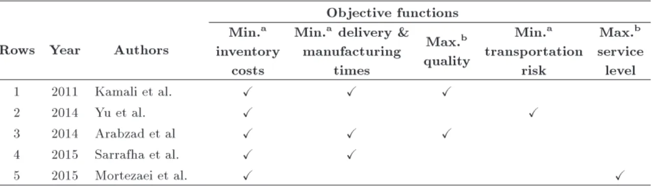
so-Table 1. Some articles related to customer satisfaction in SCM. Objective functions
Rows Year Authors
Min.a
inventory costs
Min.a delivery &
manufacturing times
Max.b
quality
Min.a
transportation risk
Max.b
service level
1 2011 Kamali et al. X X X
2 2014 Yu et al. X X
3 2014 Arabzad et al X X X
4 2015 Sarrafha et al. X X
5 2015 Mortezaei et al. X X
aMinimizing;bMaximizing.
Figure 1. Four-layer SC of the proposed model.
lutions to the multi-objective problems [28,29]. Yu et al. [30] presented a bi-objective model under un-certainty in which minimizing costs and risks are considered as the two objectives.
Literature review shows that all important factors aecting customer satisfaction, such as quality, cost, delivery, etc., are not considered together in one model (Table 1).
A new multi-product multi-period multi-objective SC model is proposed in this paper to minimize the total inventory costs while maximizing customers' sat-isfaction. The rest of this paper is organized as follows. Problem denition and mathematical formulations of the model are given in Section 3. Section 4 presents the solving procedure of the proposed model. Conclusions and further studies are presented in Section 5.
3. Problem denition
The proposed model follows two main objectives as reducing inventory costs in four-layer SC and achieving maximum customer satisfaction. Similar to Kamali et al. [22], we suppose that customer satisfaction can be
increased by minimizing failure quantity. We consider lower prices for imperfect items. Inspection and rework costs are added to the model. In addition, it is supposed that the higher level of quality can lead to an increase in time that is not pleasant for customers. This model uses the model presented by Arabzad et al. [24] considering the risk of vehicles to select the best vehicles between manufacturers and distribution centers. Also, due to the defective products, increasing customer service levels is very important. Mortezaie et al. [23] maximized service levels by minimizing the ratio of delivered items and demands. Figure 1 represents the network of four-layer SC of the model.
3.1. Notations and assumptions
To extend the mathematical model, the indices, param-eters, and decision variables adopted in this paper are as follows:
Indices
i An index for manufactured items, i = 1; 2; ; I
m An index for manufacturers, m = 1; 2; ; M
d An index for distribution center, d = 1; 2; ; D
s An index for supplier, s = 1; 2; ; S t An index for periods, t = 1; 2; ; T i0 An index for raw materials, i0 =
1; 2; ; I0
c An index for customers, c = 1; 2; ; C f An index for vehicles between
manufacturers and distribution centers, d, f = 1; 2; ; F v An index for vehicles between
distribution centers and customers, v = 1; 2; ; V
Parameters Oi
mdt Ordering cost of item i ordered from
distribution center c to manufacturer m per unit time t
RMPi0i
Usage percent of raw material i for manufacturing each unit of item i Di
mdt Demand rate of distribution center d of
item i manufactured at manufacturer m at period t
~ Di
ct Demand rate of customer c for item i
at period t Di0
smt Demand rate of manufacturer m of
item i0 which is supplied from supplier
m at period t T (P )i
mt Required time for manufacturing item
i at manufacturer m at period t T (S)fimdt Required time for transporting item i
from manufacturer m to distribution center d by vehicle f at period t T (S)vi
dct Required time for transporting item i
from distribution center d to customer c by vehicle v at period t
C(T )fimdt Shipment cost for vehicle f per item i from manufacturer m to distribution center d at period t
C(T )vi
dct Shipment cost for vehicle v per item i
from distribution center d to customer c at period t
C(Q)i
mt Quality cost per item i manufactured
at manufacturer m at period t C(P 1)fimdt Purchasing cost of perfect item i
which is shipped by vehicle f from manufacturer m to distribution center d at period t
C(P 2)fimdt Purchasing cost of imperfect item i which is shipped by vehicle f from manufacturer m to distribution center d at period t
C(P )i0
smt Purchasing cost of raw material i0
which is purchased from supplier s to manufacturer m at period t
mdtfi Lost sale cost per item i that is not delivered to distribution center d at period t
C(M)i
mt Manufacturing cost per item i for
manufacturer m at period t C(H)i
mt Inventory holding cost per unit of item
i for manufacturer m at period t C(H)i0
mt Inventory holding cost per unit of
raw material i0 for manufacturer m at
period t C(H)i
dt Inventory holding cost per unit of item
i for distribution center d at period t IRfimdt Financial loss of vehicle f risk for
shipping item i from manufacturer m to distribution center d at period t R(U)fimdt Maximum allowable risk for shipping
item i with vehicle f from manufacturer m to distribution center d at period t P (S)fimdt Probability of risk for shipping item i
with vehicle f from manufacturer m to distribution center d at period t E Nonproductive time, a constant value " A very small number
X1 Minimum defective and imperfect rate
X2 Maximum defective rate
Rfimdt Risk of vehicle f for shipping item i from manufacturer m to distribution center d at period t
Ci
dt Capacity of distribution center d for
item i at period t Ci
mt Capacity of manufacturer m for item i
at period t
Ctf Capacity of vehicle f at period t Cv
t Capacity of vehicle v at period t
Decision variables
fimdt Perfect quantity of item i shipped from manufacturer m to distribution center d by vehicle f at period t
mdtfi Defective and imperfect quantity of item i shipped from manufacturer m to distribution center d by vehicle f at period t
mdtfi Defective quantity of item i shipped from manufacturer m to distribution center d by vehicle f at period t mdtfi Imperfect quantity of item i shipped
from manufacturer m to distribution center d by vehicle f at period t which is lost sale
qfimdt Delivery quantity of item i shipped from manufacturer m to distribution center d by vehicle f at period t qvi
dct Delivery quantity of item i shipped
from distribution center d to
manufacturer m by vehicle v at period t
qi0
smt Delivery quantity of raw material
i0 shipped from supplier s to
manufacturer m at period t qi
dct Delivery quantity of item i shipped
from distribution center d to customer c at period t
Pi
mt Production quantity of item i for
manufacturer m at period t Ii
mt Inventory level of item i for
manufacturer m at period t Ii
dt Inventory level of item i for distribution
center d at period t
zmdtfi A binary decision variable; set equal to one if vehicle f delivers item i from manufacturer m to distribution center d at period t, and zero otherwise zvi
dct A binary decision variable; set equal
to one if vehicle v delivers item i from distribution center d to customer c at period t, and zero otherwise
Moreover, the assumptions involved in the problem are: I. Selecting suppliers and distributors is considered
for strategic levels;
II. Assigning products to the distribution channels and selecting the shortest routes from man-ufacturing plants to distribution centers are considered as tactical decisions;
III. Determining quantity of manufactured items per plant per period, inventory levels in distribution centers and factories, the lost sale quantity per period, the amount of raw material shipped from suppliers to manufacturers are all SC planning decisions;
IV. Manufactured items include three parts: perfect, imperfect, and defective items;
V. Manufacturers suggest lower prices for imperfect items;
VI. Lost sales are defective items;
VII. The model considers creating costs for appropri-ate levels of quality;
VIII. High number of perfect items is considered as high quality which makes customer satised; IX. Dierent vehicles can be selected for dierent
periods;
X. Purchasing costs are dierent for periods; XI. To make the model more realistic, customers'
demands are considered as fuzzy numbers. 3.2. Mathematical formulations of model Mathematical mixed-integer non-linear programming of the proposed model is as follows:
T OC =XI
i=1 M X m=1 D X d=1 T X t=1 Oi
mdt q fi mdt
qfimdt+ " !
; (1)
T SCmd= I X i=1 M X m=1 D X d=1 F X f=1 T X t=1 h
C(T )fimdtqfimdtzfimdti; (2) T SCdc=
I X i=1 D X d=1 C X c=1 V X v=1 T X t=1 C(T )vi
dct qvidctzdctvi
; (3) T BC =XI
i=1 M X m=1 D X d=1 F X f=1 T X t=1
mdtfi fimdt; (4)
T MC =
I X i=1 M X m=1 T X t=1 C(M)i
mt Pmti
; (5)
T HC =XI
i=1 M X m=1 T X t=1 C(H)i
mt Imti
+ I X i=1 D X d=1 T X t=1 C(H)i dt Idti
; (6)
T RC =XI
i=1 M X m=1 D X d=1 T X t=1 F X f=1
IRfimdt zmdtfi ; (7)
T QC =XI
i=1 M X m=1 D X d=1 T X t=1 C(Q)i
mt Pmti
; (8)
T P C = I
0
X
i0=1
S X s=1 M X m=1 T X t=1 C(P )i0
smt qi
0 smt + I X i=1 M X m=1 D X d=1 F X f=1 T X t=1 h
+XI i=1 M X m=1 D X d=1 F X f=1 T X t=1
C(P 1)fimdtfimdt; (9) min Z1=T OC + T SC + T BC + T MC + T HC
+ T RC + T P C + T QC; (10)
min Z2= I X i=1 M X m=1 D X d=1 F X f=1 T X t=1
mdtfi ; (11)
min Z3= I X i=1 M X m=1 T X t=1
T (P )i
mt Pmti
+XI
i=1 M X m=1 D X d=1 T X t=1 F X f=1
T (S)fimdt zfimdt
+ I X i=1 D X d=1 C X c=1 V X v=1 T X t=1
T (S)vi cdtzcdtvi
+E;
(12) max Z4=
PI i=1 PM m=1 PD d=1 PF f=1 PT t=1 fimdt PI i=1 PM m=1 PD d=1 PT
t=1 Dmdti
;
(13) min Z5=
I X i=1 M X m=1 D X d=1 F X f=1 T X t=1 Rfi
mdt Zmdtfi
; (14) S.t.:
Ii
m;t 1+ Pmti
Ci
mt; 8 i; m; t; (15)
Ii dt+
M
X
m=1
qfimdt= Ci
dt; 8 f; i; d; t; (16)
qmdtfi zfimdt Ctf; 8 i; m; d; t; f; (17) qvi
dct zdctvi
Cv
t; 8 i; c; d; t; v; (18)
D X d=1 V X v=1 qvi
dct ~Dict; 8 i; c; t; (19)
D X d=1 V X v=1 qvi dct M X m=1
qmdtfi fimdt; 8 f; i; c; t; (20)
F
X
f=1
zmdtfi = 1; 8 i; m; d; t; (21)
V
X
v=1
zvi
dct= 1; 8 i; c; d; t; (22)
S
X
s=1
qi0
smt RMPi
0i
Pi
mt; 8 i0; i; m; t; (23)
Pi
mt= Imti + D
X
d=1
qfimdt; 8 f; i; m; t; (24) Rfimdt= P (S)fimdt IRfimdt; 8 f; i; m; d; t; (25) Rfimdt zmdtfi R(U)fimdt; 8 f; i; m; d; t; (26) mdtfi = fimdt+ mdtfi ; 8 f; i; m; d; t; (27)
F
X
f=1
fimdt Di
mdt; 8 f; i; m; d; t; (28)
qmdtfi = mdtfi + fimdt; 8 f; i; m; d; t; (29) mdtfi X1 qmdtfi ; 8 f; i; m; d; t; (30) fimdt (1 X1) qfimdt; 8 f; i; m; d; t; (31) mdtfi X2 mdtfi ; 8 f; i; m; d; t; (32) mdtfi (1 X2) fimdt; 8 f; i; m; d; t; (33) fimdt;mdtfi ; mdtfi ; fimdt; qmdtfi ; Pi
mt; qi
0
smt; qdctvi;
Ii
mt; Idti ; Ii
0
mt 0; (34)
zfimdt; zvi
mdt; zmti 2 f0; 1g: (35)
Eq. (1) calculates the total ordering costs of distribution center d. Eqs. (2) and (3) represent transportation costs of vehicles f and v, respectively. Eq. (4) shows the lost sale costs of defective items. Eq. (5) calculates manufacturing costs. Total inventory costs of manufactured items and raw materials are obtained by Eq. (6). Financial losses resulting from transportation risk are obtained by Eq. (7). Eq. (8) represents the providing quality costs. Formula Eq. (9) calculates the total purchasing cost of SC. The total inventory costs of SC are obtained by Eq. (10). Quality function is represented in Eq. (11). The third objective aims to maximize customer satisfaction by minimizing manufacturing and shipping costs which are obtained by Eq. (12). Eq. (13) represents service levels. The fth objective function minimizes transportation risks and is calculated by Eq. (14). Eqs. (15) to (34) are constraints of the proposed models. Constraints (15) and (16) show delivery quantity and inventory levels which should be equal to the capacity of manufacturers and distributors, so delivery quantities are less than or equal to capacities represented in Constraints (17)
and (18). Constraint (19) shows that delivery quantity from distribution centers to customers is equal to or less than customers' demands. Constraint (20) repre-sents the balancing equation for distribution centers. Constraints (21) and (22) show that only one type of vehicle can be selected for each item at every period in each channel. It is obvious that raw materials delivered to manufacturers should be equal to or more than their needs. This constraint is represented in Eq. (23). Quantity of manufactured items is equal to inventory levels and delivery quantity. This constraint is shown in Constraint (24). Constraint (25) calculates risk levels. The maximum allowable risk is obtained by Constraint (26). Quantity of perfect items should be less than demands. This limitation is represented by Constraint (28). Constraint (29) shows delivery quantity consisting of perfect, imperfect, and defective items. This model considers minimum rates for defec-tive and imperfect items shown in Eqs. (30) to (33). The two remaining equations dene the value ranges of variables.
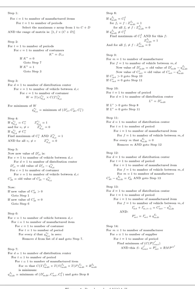
4. Solving procedure of the proposed model The NSGA II algorithm [3] is developed to solve the proposed multi-objective model. Moreover, the "-constraint method is employed to validate the obtained results. Finally, some numerical examples are gener-ated to analyze and compare the solving methods. 4.1. "-constraint method
Abounacer [31] expressed that the "-constraint method solves a set of constrained single-objective problems Pk("), " = ("1; ; "k 1; "k+1; ; "m) obtained by
choosing one objective, fk, as the only objective to
optimize and incorporate inequality constraints for the remaining objectives of the form fi ", i =
1; ; k 1, k = 1; ; m. The set of problems, Pk("), is obtained by assigning dierent values to the
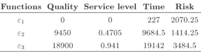
components of the "-vector. In the proposed model, minimizing the total costs of SC is selected as the main objective function and other functions are considered as constraints. By assessing dierent combinations provided by values in "-vectors, the best combination has been obtained. Table 2 represents "-vectors of the four remaining objective functions.
Dierent combinations provided from "-vectors and SC costs are examined for these combinations. Due to the large number of combinations, just a number
Table 2. "-vectors for objective functions. Functions Quality Service level Time Risk
"1 0 0 227 2070.25
"2 9450 0.4705 9684.5 1414.25
"3 18900 0.941 19142 3484.5
of solutions for cost function are shown in Table 3 for the cost function of SCM in one of the provided examples. As obvious, the best combination is the one that minimizes costs to the extent that the variables get reliable values in the problem, not zero values as highlighted in Table 3.
4.2. Non-dominant sorting genetic algorithm NSGA-II algorithm is one of the most applicable algorithms to solve multi-objective optimization prob-lems [24]. NSGA-II generates a parent population of size nP op. Then, the objective values are evaluated by using an evaluation function during several generations. To create Pareto fronts, the population is ranked based on non-dominant sorting procedures. Each individual of the population obtains a rank based on its level (1 is the best level, 2 is the second best level, and so on). The crowding distance between members is obtained for each front. First, a binary tournament selection operator is used which helps to select two members among the population. Next, a new population of ospring with the size of n is created by using simulated binary crossover (SBX) operator. It is used to create the population consisting of the current and the new population of size (nP op + n). Finally, a population of nP op size is obtained by sorting. The new population is used to generate the next new ospring by repeating these steps until the stopping condition is met. 4.2.1. Encoding and decoding the algorithm
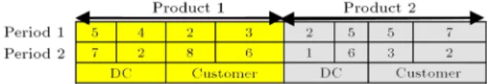
A proper chromosome representation can lead to more ecient performance of NSGA-II. In many inventory controls and SC problems, to produce a proper chromo-some in the initial population, the relationship between dierent levels of the SC is considered as dierent parts of chromosomes. Altiparmak et al. [32] proposed an illustration of chromosomes, considering a three-layer SC. They also proposed a repair algorithm, which is used when the total capacity of opened DCs or plants is not enough to meet customer demands. A representation of chromosome with dierent sections of SC in the proposed model along with a two-layer SC with two products, two raw materials, two suppli-ers, manufactursuppli-ers, distributors and customsuppli-ers, which consists two strings, is shown in Figure 2.
Given that, a random method to produce the initial population of chromosomes without a proper repair algorithm may lead to an infeasible solution.
To be more specic, in this paper, a chromosome consists of one section. This section is organized according to the relationship between distributors and customers with the length of I(D + C) represented by T strings, where T is a xed number of periods. In this method, each gene on the proposed chromosome is not permuted randomly (according to distributors' capacities and customers' demands) from [1; I(C +
Table 3. Cost function values for dierent combinations of other functions' "-vectors. "
(quality) " (service
level) " (time)
" (risk)
Total cost value
" (quality)
" (service
level) " (time)
" (risk)
Total cost value 9450 0 9684.5 2070.25 83268330 9450 0.4705 9684.5 2777.375 84833740 9450 0 9684.5 2777.375 82782820 9450 0.4705 9684.5 3484.5 84877630
9450 0 9684.5 3484.5 83268330 9450 0.4705 19142 2070.25 85431890
9450 0 19142 2070.25 83268330 9450 0.4705 19142 2777.375 84883720
9450 0 19142 2777.375 82749290 9450 0.4705 19142 3484.5 84830430
9450 0 19142 3484.5 82747410 18900 0 9684.5 2070.25 83268330
9450 0.4705 9684.5 2070.25 85431890 18900 0 9684.5 2777.375 82720390 9450 0.4705 9684.5 2777.375 84833740 18900 0 9684.5 3484.5 82720390 18900 0.4705 19142 2070.25 85431890 18900 0 19142 2070.25 83268330 18900 0.4705 19142 2777.375 84864790 18900 0 19142 2777.375 82720390
18900 0.4705 19142 3484.5 84864790 18900 0 19142 3484.5 82720390
18900 0.4705 9684.5 2777.375 84820870 18900 0.4705 9684.5 2070.25 85431890
| | | | | 18900 0.4705 9684.5 3484.5 84918810
Figure 2. Sample of chromosome representation.
Figure 3. Chromosome representation.
D)]. Figure 3 represents an example of a chromosome for a supply chain which includes two distributors, customers, products, and periods. To enhance the feasible solutions according to the main goal of this model for satisfying customers' demand, the maximum allele value is selected. Then, the delivery quantity between customers and distribution centers is obtained. After selecting the maximum allele value, a heuristic method is proposed to evaluate the tness value of chromosomes. Using the steps of the proposed method, feasible chromosomes that satisfy all constraints except Constrain (15) are generated. To t the problem
at hand, Pasandideh et al. [17] used encoding and decoding procedure and modied it based on the model formulation at hand.
According to a gene selected with the maximum number (customer with most demands or distribution center with high capacity) of chromosomes, there are some decisions as follows:
- Step 1. The best distribution centers are allocated to customers according to transportation costs, time between distribution centers and selected customer. Regarding the customers' demand rates, distribution center's capacity, vehicle deliverable quantities while minimizing the ratio of received items to demand rate, the number of their deliveries is examined. After updating unsatised demands and distribution center's capacity, if capacities are more than zero, this step will be repeated until the capacity or total demands of customers reach zero. The delivery quantities between customers and DCs, shortages and distribution centers' inventories will be obtained in this step. This step meets Constraints (18), (19), and (23);
- Step 2. Considering the inventory and shortage levels of manufacturing plants as equal to zero and removing unselected distribution centers from the list, manufacturing plants will be selected according to manufacturing and transportation time and costs. There are many factors aecting the delivery quan-tity between manufacturers and distributors. The capacity of distributors and manufacturers is one of these factors. Moreover, vehicles will be selected according to their capacities and risk. Inventory levels of plants, delivery quantities, perfect and imperfect items, and defective product numbers
are examined while minimizing the ratio of the delivery quantity and demand between plants and distributors. Constraints (16)-(17) and (20)-(33) are met in this step;
- Step 3. According to purchase prices, allocated suppliers, plants, etc., the number of manufactured items, and percentage of used raw material for each product and delivery quantities are examined. Constraint (23) is met in this step.
4.2.2. Evaluation
In the proposed model, the maximum allowed risk limitation may cause infeasible solutions. Eq. (15) is another constraint which may cause infeasibility of solutions because it is not satised by using the proposed steps of heuristic methods. In order to avoid the solutions that do not satisfy these constraints, the penalty function approach is employed by Mousavi et al. [27]. These penalty functions are added to the objective functions based on the sum of two squared of violation of these constraints which can be referred to [17]. Eqs. (36) and (37) show two employed violation formulas:
Eq1=
h
Rmdtfi zfimdt R(U)fimdti4; (36) Eq2= Im;t 1i + Pmti
Ci
mt
4: (37)
Using penalty functions, the tness function vector is evaluated as in Eqs. (38) and (39):
If the individual is not in a feasible region: Penalty = Eq2
1+ Eq22: (38)
If the individual is in a feasible region: Penalty = 0;
Fitness function vector= 8 > > > > > > < > > > > > > :
Z1+penalty function
Z2+penalty function
Z3+penalty function
Z4+penalty function
Z5+penalty function
(39) 4.2.3. Crossover operator
The crossover is done to explore new solution spaces. The SBX operator [32] uses a probability distribution around two parents to create two children solutions. Unlike other real-parameter crossover operators, SBX uses a probability distribution [33].
4.2.4. Mutation operator
Mutation is used to prevent the premature convergence and explore new solution spaces. In this study, polynomial mutation operator is used. The probability
distribution is a polynomial function. The probability of creating a solution closer to the parent is more than the probability of creating one away from it. The shape of the probability distribution is directly controlled by an external parameter, and the distribution is not dynamically changed with iterations [34].
4.2.5. Parameter tuning of NSGA-II
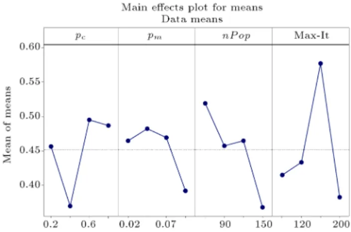
Since the parameters of NSGA-II play an important role in the quality of an obtained solution, in this paper, Taguchi method is used for tuning. The Taguchi method is implemented to tune the parameters of the algorithm. The reason why Design Of Experiment (DOE) is selected, rather than the other approaches to conduct an experiment, is that it has a system-atic planning of experiments. One of the important steps involved in Taguchi's technique is a selection of orthogonal array. This method is an ecient procedure that is developed as an alternative to the full factorial experimental design method [35]. There are two suggested ways in Taguchi method to analyze the results. First, analysis of variance that is used for experiments that are repeated once; second, Signal-to-Noise ratio (S=N) that is used for experiments with multiple runs [36]. In the second method, a statistical measurement, S=N, is used to evaluate the performance. Figures 3 and 4 represent mean of mean and S=N ratios for this paper. Taguchi categorizes objective functions into three groups: the smaller the best type, the larger the best type, and nominal-is-the best type. Since cost function is of smaller-the-better type, its corresponding S=N ratio is as in Eq. (40):
S=N = 10 log10 y S
2
: (40)
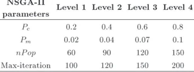
There are four parameters to be calibrated [37]; population size (nP op), number of iterations (max-iteration), and crossover, and mutation rates (Pc and
Pm). These parameters with four levels are shown
in Table 4 to run the experiments based on Taguchi design.
Table 5 represents Taguchi Experimental design for NSGA-II parameters.
The nal analysis of experimental design is shown in Figures 5 and 6.
Finally, optimum levels for NSGA-II parameters are obtained as shown in Table 6.
Table 4. Level of NSGA-II parameters. NSGA-II
parameters Level 1 Level 2 Level 3 Level 4
Pc 0.2 0.4 0.6 0.8
Pm 0.02 0.04 0.07 0.1
nP op 60 90 120 150
Table 5. Taguchi experimental design for NSGA-II parameters.
Run
order Pc Pm nP op Max-iteration Fitness 62
1 0.2 0.1 60 100 0.471691
2 0.2 0.04 90 120 0.563501
3 0.2 0.07 120 150 0.564812
4 0.2 0.02 150 200 0.226407
5 0.4 0.02 90 150 0.496602
6 0.4 0.04 60 200 0.351070
7 0.4 0.07 150 100 0.356001
8 0.4 0.1 120 120 0.276391
9 0.6 0.02 120 200 0.540974
10 0.6 0.04 150 150 0.538279
11 0.6 0.07 60 120 0.543718
12 0.6 0.1 90 100 0.357596
13 0.8 0.02 150 120 0.350830
14 0.8 0.04 120 100 0.474895
15 0.8 0.07 90 200 0.411590
16 0.8 0.1 60 150 0.709102
Table 6. NSGA-II optimum parameters. Pc Pm nP op Max-It
0.4 0.1 150 200
4.3. Numerical results
Consider a multi-period SC with multiple suppliers, manufacturers, distribution centers, and customers. The suppliers produce more than one raw material and plants manufacture several items under customer demand uncertainty. Some problem instances are generated as shown in Table 7.
Parameters' corresponding ranges of the men-tioned problem instances are shown in Table 8. These parameters are generated randomly by using some related literature reviews.
As mentioned before, the demands of customers
Figure 5. Plots of main eects for S=N ratios of NSGA-II.
Figure 6. Plots of main eects for means of NSGA-II.
are considered as trapezoidal fuzzy numbers to make the model more realistic while considering the uncer-tainty. These fuzzy data are defuzzied after gener-ating, and then are used. To do this, the mean-max membership method is employed. Interested readers are referred to [38] to read more.
These instances are rstly solved by "-constrain method by GAMS software on a corei5 processor, 4 G RAM and 2.4 GHz PC. The problem is computation-ally intractable and GAMS was unable to nd solutions
Table 7. Generated problem instances.
Problem no.
1 2 3 4
Raw materials 2 2 2 2
Manufactured items 2 2 2 2
Suppliers 2 2 4 4
Manufacturers 2 2 2 2
Distribution centers 2 3 3 3
customers 2 2 2 4
Number of vehicles between plants and DCs 2 2 2 2 Number of vehicles between DCs and customers 2 2 2 3
Table 8. Parameters ranges for SC.
Parameter Range Parameter Range Parameter Range
Oi
mdt: [400,510] C(P 1)fimdt: [500,570] P (S)fimdt: [0.25,0.6]
RMPi0i: [40,50] C(P 2)fi
mdt: [400,550] Ctv: 250
Di
mdt: [720,900] C(P )i
0
smt: [300,370] Cdti : [750,840]
Di
ct: [1000,1900] fimdt: [200,270] Cmti : [2000,2800]
Di0
smt: [650,850] C(M)imt: [400,500] Ctf : 250
T (P )i
mt: [1,2] C(H)imt: [650,900] E : 3
T (S)fi
mdt: [5,7] C(H)i
0
mt: [800,950] X2 : 0.03
T (S)vi0
dct: [5,7] C(H)idt: [250,400] X1 : 0.02
C(T )fimdt [600,660] C(T )ft : [100,150] R(U)fimdt: [300,390]
C(T )vi
dct [500,560] IRfimdt: [270,300] C(Q)imt [700,950]
Table 9. Computational results of the "-constrain method and NSGA-II algorithm. Problem
no.
"-constraint NSGA-II
Z1 Z2 Z3 Z4 Z5 CPU
time Z1 Z2 Z3 Z4 Z5
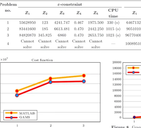
CPU time 1 55628950 123 4241.747 0.467 1975.500 330 (s) 64671320 141 4601.500 0.402 2010.300 252 2 83441600 185 6613.481 0.470 2442.250 1015 (s) 90510100 201 6923.359 0.422 2523.102 335 3 84820870 345.825 6860 0.470 2653.750 1023 (s) 967704000 403 7001.200 0.426 2823.840 387
4 Cannot
solve
Cannot solve
Cannot solve
Cannot solve
Cannot
solve | 100895100 467 7433.550 0.426 2825.500 831
Figure 7. Graphical comparison of solving methodologies in terms of cost function.
to larger than medium-sized problems. Therefore, NSGA-II was employed to solve them by MATLAB. The comparison of these methodologies is shown in Table 9 and Figures 6 to 11.
Figures 7-12 present the comparison of method-ologies between ve objective functions of the proposed models in Section 4. Figure 8 shows CPU time of solving methods. This gure shows that NSGA-II is applicable to solve the fourth problem instance, not solved by "-constraint method. Since this new model is more complicated with ve objectives and more num-ber of constraints, NSGA-II is applicable to medium-sized problems and represent reasonable solutions.
Figure 8. Graphical comparison of solving methodologies in terms of CPU time.
Figure 9. Graphical comparison of solving methodologies in terms of quality function.
Figure 10. Graphical comparison of solving methodologies in terms of service level function.
Figure 11. Graphical comparison of solving methodologies in terms of time function.
Figure 12. Graphical comparison of solving in terms of risk function.
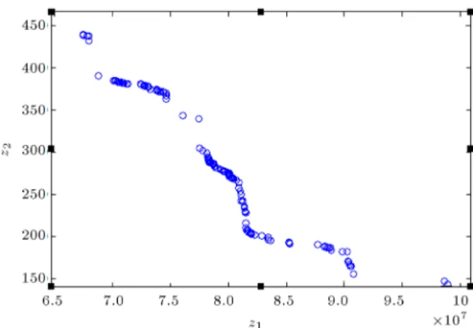
When a NSGA-II is used for optimizing a multi-objective mathematical model, a set of Pareto solutions is provided. The Pareto solutions obtained by every iteration while using suggested algorithm are shown in Figures 13-16. These gures show the trade-o between cost functions and other objective functions for the third problem instance each in one curve.
The most important issue about each meta-heuristic algorithm is the best value. After more than one hundred runs, the best combination is obtained as Table 9. The convergence path of NSGA-II is plotted in Figure 17.
To evaluate the performances of the proposed approaches, three standard metrics of multi-objective algorithms are applied. In order to compare the obtained results and objective functions' behavior di-versity, CPU time and NOS metrics are used for Pareto
Figure 13. Pareto-optimal solution of NSGA-II for minimizing cost and defective and imperfect items.
Figure 14. Pareto-optimal solution of NSGA-II for minimizing cost and time.
Figure 15. Pareto-optimal solution of NSGA-II for minimizing costs and risk.
solutions. Diversity measures the extension of the Pareto front, in which the bigger value is better [39]. NOS counts the number of Pareto solutions in the Pareto optimal front in which the bigger value is better [40]. CPU time shows the time of running the approaches to reach near-optimum solutions. Table 10 represents the spread of curves for "-constraint and
Table 10. Comparison of the obtained results of the "-constrain method and NSGA-II algorithm. Problem
no.
"-constraint NSGA-II
Diversity CPU time (s) NOS Diversity CPU time (s) NOS
1 8.8609E+08 330 64 8.1872E+08 252 72
2 4.2341E+08 1015 63 3.0681E+08 335 72
3 3.4912E+08 1023 63 3.2601E+08 387 74
4 | Not solved | 2.6654E+08 831 70
Figure 16. Pareto-optimal solution of NSGA-II for minimizing cost and maximizing service level.
Figure 17. The convergence path of the best result by NSGA-II.
NSGA-II. This table also shows CPU time consumed to solve problem instances by the two mentioned methodologies and NOS metrics.
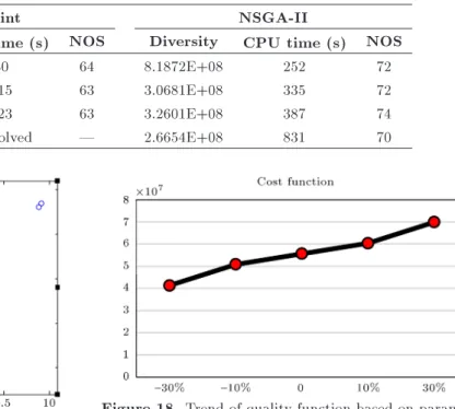
Sensitivity analysis is utilized to asses parameters' eects on objective functions. The value of the parameters is changed in the interval ({30%, 30%). Sensitivity analysis results show that the most eective parameter on cost function is Di
mdt. Parameters
RMPi0i
and P s are the most eective ones in quality and time functions, respectively. T (P )i
mt and IR are
two parameters which aect risk function. Figures 18-20 show the most eective parameter in cost and time objective functions.
Figure 18. Trend of quality function based on parameter Di
mdt.
Figure 19. Trend of cost function based on parameter RMPi0i.
Figure 20. Trend of risk function based on parameter P s.
5. Conclusion and future research
In this paper, a new multi-objective mixed-integer nonlinear programming was presented for a multi-item multi-period SCM problem. It was assumed that demand rates are fuzzy values.
and minimize the total costs. An exact method and a meta-heuristic algorithm were used to solve the proposed model. Furthermore, a Taguchi method was utilized to calibrate NSGA-II parameters. The obtained results show the validity of the suggested solving methods. Four numerical examples were solved and compared by two solving methods based on two measures: value of objective functions and CPU time. While "-constraint was unable to solve the last prob-lem, NSGA-II was able to solve it and provide Pareto front solutions.
As for further research directions, it is suggested to consider these assumptions:
Utilizing engineering economic techniques, such as ination rate, to calculate the costs exactly; Considering networks of suppliers and distributors
instead of layers of some nodal enterprises;
Using green supply chain concepts to reduce en-vironment's pollution; performing a real-situation case study;
Utilizing some other meta-heuristic algorithms and comparing the obtained results to nd the best solving method.
References
1. Pasandideh, S.H.R., Niaki, S.T.A. and Asadi, K.
\Optimizing a bi-objective multi-product multi-period three layer supply chain network with warehouse reli-ability", Expert Systems with Applications, 42(5), pp. 2615-2623 (2015).
2. Shirani, A., Danaei, H. and Shirvani, A. \A study on
dierent factors inuencing customer satisfaction on industrial market", Management Science Letters, 4(1), pp. 139-144 (2014).
3. Deb, K., Agrawal, S., Pratap, A. and Meyarivan, T. \A
fast elitist non-dominated sorting genetic algorithm for multi-objective optimization: NSGA-II", In Proceed-ings of Parallel Problem Solving, 1917, pp. 489-858 (2000).
4. Abounacer, R., Rekik, M. and Renaud, I. \An
ex-act solution approach for multi-objective location-transportation problem for disaster response", Com-puters and Operations Research, 41, pp. 25-39 (2014).
5. Harris, W. \How many parts to make at once?
Fac-tory", The Magazine of Management, 10, pp. 135-152 (1913).
6. Miller, L. \A multi-item inventory model with joint
backorder criterion", Operations Research, 19(6), pp. 1467-1476 (1971).
7. Kirkpatrick, S., Gelatt, C.D. and Vecchi, M.P.
\Op-timization by simulated annealing", Science, 220, pp. 671-680 (1983).
8. Das, K., Roy, T.K. and Maiti, M. \Multi-item
inven-tory model with quantity-dependent inveninven-tory costs and demand-dependent unit cost under imprecise ob-jective and restrictions: a geometric programming approach", Production Planning and Control, 11(8), pp. 781-788 (2000).
9. Clark, A. and Scarf, H. \Optimal policies for a
multi-layer inventory problem", Management Sciences, 6(4), pp. 475-490 (1960).
10. Bessler, S. and Veinott, A.F. \Optimal policy for a
dynamic multi-layer inventory model", Naval Research Logistics Quarterly, 13(4), pp. 355-389 (1965).
11. Goyal, S.K. \An integrated inventory model for a
single supplier-single customer problem", International Journal of Production Research, 15(1), pp. 107-111 (1977).
12. Hsiao, J.M., and Lin, C. \A buyer-vendor EOQ
model with changeable lead time in supply chain", International Journal of Advanced Manufacturing and Technology, 26(7), pp. 917-921 (2005).
13. Abdul-Jalbar, B., Gutierrez, J.M. and Sicilia, J.
\Poli-cies for a single-vendor multi-buyer system with nite production rate", Decision Support Systems, 46(1), pp. 84-100 (2008).
14. Taleizadeh, A., Niaki, S.T.A. and Makui, A.
\Multi-product multiple-buyer single-vendor supply chain problem with stochastic demand, variable lead-time, and multi-chance constraint", Expert Systems with Applications, 39(26), pp. 5338-5348 (2012).
15. Sadeghi, J., Mousavi, S.M., Niaki, S.T.A. and Sadeghi,
S. \Optimizing a multi-vendor multi-retailer ven-dor managed inventory problem: Two tuned meta-heuristic algorithms", Knowledge-Based Systems, 50, pp. 159-170 (2013).
16. Varyani, A., Jalilvand-Nejad, A. and Fattahi, P.
\De-termining the optimum production quantity in three-layer production system with stochastic demand", In-ternational Journal of Advanced Manufacturing Tech-nology, 72(1), pp. 119-133 (2014).
17. Pasandideh, S.H.R., Niaki, S.T.A. and Asadi, K.
\Bi-objective optimization of a multi-product multi-period three-layer supply chain problem under uncertain en-vironments: NSGA-II and NRGA", Information Sci-ences, 292(7), pp. 57-74 (2015).
18. Pasandideh, S.H.R., Niaki, S.T.A. and Asadi, K.
\Optimizing a bi-objective multi-product multi-period three layer supply chain network with warehouse reli-ability", Expert Systems with Applications, 42(5), pp. 2615-2623 (2015).
19. Sadeghi, J. and Niaki, S.T.A. \Two parameter
tuned multi-objective evolutionary algorithms for a bi-objective vendor managed inventory model with trapezoidal fuzzy demand", Applied Soft Computing, 30, pp. 567-576 (2015).
20. Sarrafha, K., Rahmati, S.H.A., Niaki, S.T.A. and
production, and distribution problem of a multi-layer supply chain network design: a new tuned MOEA", Computers & Operations Research, 54, pp. 35-51 (2015).
21. Suchanek, P., Richter, J. and Kralova2, M.
\Cus-tomer satisfaction" product quality and performance of companies", Review of Economic Perspectives -Narodohospodasky Obzor, 14(4), pp. 329-344 (2015).
22. Kamali, A., Fatemi Ghomi, S.M.T. and Jolai, F. \A
multi-objective quantity discount and joint optimiza-tion model for coordinaoptimiza-tion of a single-buyer multi-vendor supply chain", Computers and Mathematics with applications, 62(20), pp. 3251-3262 (2011).
23. Mortezaei, N., Zulkii, N. and Nilashi, M.
\Trade-o analysis f\Trade-or multi-\Trade-objective aggregate pr\Trade-oducti\Trade-on planning", Journal of Soft Computing and Decision Support System, 2(2), pp. 1-4 (2015).
24. Arabzad, S.M., Ghorbani, M.R. and
Tavakkoli-Moghaddam, R. \An evolutionary algorithm for a new multi-objective location-inventory model in a distribution network with transportation modes and third-party logistics providers", International Journal of Production Research, 53(4), pp. 1038-1050 (2014).
25. Sadeghi, J., Sadeghi, S. and Niaki, S.T.A. \Optimizing
a hybrid vendor-managed inventory and transporta-tion problem with fuzzy demand: An improved particle swarm optimization algorithm", Information Sciences, 272, pp. 126-144 (2014).
26. Sadeghi, J. and Niaki, S.T.A. \Two parameter
tuned multi-objective evolutionary algorithms for a bi-objective vendor managed inventory with trapezoidal fuzzy demand", Application of Soft Computing, 30, pp. 567-576 (2015).
27. Mousavi, M., Sadeghi, J., Niaki, S.T.A. and Tavanad,
M. \A bi-objective inventory optimization model un-der ination and discount using tuned Pareto-based algorithms: NSGA-II, NRGA, and MOPSO", Applied Soft Computing, 43, pp. 57-72 (2016).
28. Hassanzadeh, S. and Guoqing Zhang, A. \A
multi-objective facility location model for closed-loop supply chain network under uncertain demand and return", Applied Mathematical Modelling, 37(6), pp. 4165-4176 (2013).
29. Saar, M., Shakouri, H. and Jafar Razmi, G. \A
new multi objective optimization model for designing a green supply chain network under uncertainty", International Journal of Industrial Engineering Com-putations, 6(1), pp. 15-32 (2015).
30. Yu, M.C. and Goh, M. \A multi-objective approach to
supply chain visibility and risk", European Journal of Operational Research, 233(1), pp. 125-130 (2015).
31. Abounacer, R., Rekik, M. and Renaud, I. \An
ex-act solution approach for multi-objective location-transportation problem for disaster response", Com-puters and Operations Research, 41, pp. 25-39 (2014).
32. Altiparmak, F., Gen, M., Lin, L. and Paksoy, T.
\A genetic algorithm approach for multi-objective optimization of supply chain networks", Computers & Industrial Engineering, 51(16), pp. 196-215 (2006).
33. Deb, K. and Agrawal, S. \A Niched-Penalty Approach
for Constraint Handling in Genetic Algorithms", Arti-cial Neural Nets and Genetic Algorithms, pp. 235-243 (1999).
34. Kannan, S., Baskar, S. and Murugan, P. \Application
of NSGA-II algorithm to single-objective transmission constrained generation expansion planning", IEEE Transactions on Power System, 24(4) pp. 1790-1797 (2009).
35. Kaladhar1, M., Subbaiah, K.V., Srinivasa Rao, Ch.
and Narayana Rao, K. \Application of Taguchi ap-proach and utility concept in solving the multi-objective problem when turning AISI 202 austenitic stainless steel", Journal of Engineering Science and Technology Review, 4(1), pp. 55-61 (2011).
36. Mousavi, S.M., Hajipour, V., Niaki, S.T.A. and Alikar,
N. \Optimizing multi-item multi-period inventory con-trol system with discounted cash ow and ination: Two calibrated meta-heuristic algorithms", Applied Mathematical Modeling, 37(1), pp. 2241-2256 (2013).
37. Roy, R., A Primer on the Taguchi Method, Society of
Manufacturing Engineers, New York, USA (1990).
38. Fraley, S., Oom, M., Terrion, B. and Date, J.Z. \Design
of experiments via Taguchi methods: orthogonal ar-rays", USA: The Michigan Chemical Process Dynamic and Controls Open text Book (2006).
39. Zitzler, E. and Thiele, L. \Multiobjective optimization
using evolutionary algorithms - A comparative case study", Parallel Problem Solving from Nature, Ger-many, pp. 292-301 (1998).
40. Zitzler, E., Laumanns, M. and Thiele, L. \SPEA2:
Improving the strength Pareto evolutionary algorithm, Evolutionary Methods for Design", Optimization and Control with Applications to Industrial Problems, Greece, pp. 95-100 (2001).
Biographies
Shabnam Fazli Besheli received her BSc degree in Industrial Engineering from the Iran University of Science and Technology, Behshar Branch in 2011. She is currently a student with a master degree in Industrial Engineering in Mazandaran Institute of Technology. Her research interests are multi-objective multi-product multi-period supply chain problems and customer Satisfaction and transportation risks. Ramezan Nemati Keshteli holds BS, MS, and PhD degrees in Industrial Engineering from Khajeh Nasir University of Technology, Isfahan University of Technology and Tarbiat Modares University, respec-tively. His research interests include statistical quality
control, multivariate decision-making, and articial intelligence.
Saeed Emami holds BS, MS, and PhD degrees in Industrial Engineering from Isfahan University of Technology. His research interests include scheduling, multiple criteria decision-making, and facility location.
Seyedeh Mansooreh Rasouli received her BSc de-gree in Industrial Engineering from the Babol Noshir-vani University of Technology in 2013. She is currently a student with a master degree in Industrial Engi-neering in Mazandaran Institute of Technology. Her research interests include optimizing multi-objective multi-period location-inventory control problem.