Large Eddy Simulation of Separated Flow over a Wall-Mounted Cube

Flow over a Wall-Mounted Cube

M. Farhadi

1

and M. Rahnama

Large eddy simulation of ow over a wall-mounted cube in a channel was performed at a Reynolds number of 40000. The structure function modeling of the subgrid-scale stress terms was used with three slightly varying versions of its selective type. The convective terms were discretized using a QUICK scheme, along with a relatively coarse grid. A series of time-averaged velocities and turbulent stresses were computed and compared with experimental data to examine the performance of these models. The structure function model yielded decient mean ow structure and turbulence statistics compared with the selective structure function. While none of these models could reproduce experimental results exactly, the results of time-averaged streamline plots and turbulent kinetic energy for one of the selective structure function models showed less discrepancy with experimental data compared with other models. It was shown that implementation of a wall function does not improve the results considerably and, in general, with a coarse grid resolution, it is possible to obtain some reasonable results as compared to the experiment.

INTRODUCTION

Turbulent ow past three-dimensional blu bodies has attracted much attention because of the wide range of engineering applications, such as electronic boards and the ow around tall buildings. Accurate prediction of ow characteristics is required in such applications to be sure of a safe and economical design. Numerical simulation of ow in such congurations is capable of revealing detailed information, which is much more necessary than its experimental counterpart.

A wall-mounted cube subjected to the ow in a channel is a basic geometry (Figure 1) with some important phenomena, such as ow separation with partial reattachment, wake ow periodicity and large-scale turbulence structures. There is a vast amount of literature about experiments undertaken for this geometry [1-6]; among them being the comprehensive work of Martinuzzi and Tropea [5] for a Reynolds number of 40000. Their ow picture given in Figures 2a and 3a shows the very complex ow nature, in spite of its simple geometry. As observed in these gures, the

1. Department of Mechanical Engineering, Shahid Bahonar University of Kerman, Kerman, I.R. Iran.

*. Corresponding Author, Department of Mechanical En-gineering, Shahid Bahonar University of Kerman, Ker-man, I.R. Iran.

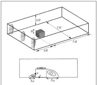
Figure 1.

Geometry of computational domain and schematic of recirculation zones.

ow separates in front of the cube; in the mean there is a primary separation vortex and, also, a secondary one, while, instantaneously, up to three separation vortices were detected. The main vortex bends as a horseshoe vortex around the cube into the wake; having a typical converging-diverging behavior. The ow separates at the front corners of the cube on the roof and sidewalls. In the mean, it does not

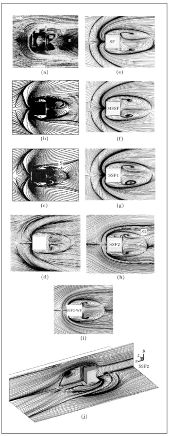
Figure 2.

Time-averaged computations of streamline plots at the oor of the channel by (a) Experiments [5], (b) OEM model [10], (c) LDKM model [10], (d) Computations of Shah and Ferziger [9], (e) SF model, (f) MSSF model, (g) SSF1 model, (h) SSF2 model, (i) SSF2-WF model, all at Re = 40000 and (j) SSF2 model at Re = 3200.

Figure 3.

Comparison of time-average streamline plots at planez= 0 obtained from (a) Experimental data and (b-f) Present computations.

reattach on the roof. A large separation region develops behind the cube that interacts with the horseshoe vortex. Numerical investigation of such complex ow conguration is a challenge for researchers in the eld of computational uid mechanics.

Various authors have done numerical predictions of turbulent ow over a wall-mounted cube in a channel using Direct Numerical Simulation (DNS), Large Eddy Simulation (LES), Reynolds-Averaged Navier-Stockes equations (RANS) [7] and, recently, Detached Eddy Simulation (DES) [8]. In fact, several international workshops have been held on this ow conguration [7]. The two Reynolds numbers used in these computations were 3000 and 40000. These workshops indicated that LES is able to predict the main characteristics of such ow conguration more accurately than RANS and much more cheaply than DNS computations. The subgrid-scale models used in these computations were Smagorinsky, dynamic and mixed models. Many of these LES computations used a ne grid resolution (more than 106_{nodes for low Reynolds number). Shah}

and Ferziger [9] reported LES simulation of ow around a cubic obstacle at Re = 40000 with 1926496

grid points. Using no wall function for the region near the wall, these simulations approach Direct Numerical Simulation (DNS), resolve the near-wall streaks and may be described as Quasi-DNS (QDNS) [10]. In such circumstances, the inuence of the Subgrid-Scale (SGS) model is then small. Although these LES were carried out with considerable success, the extension of this kind of simulation to a higher Reynolds number and more complex geometry implies very high computational costs.

Recently, Iaccarino et al. [11] studied the accuracy of unsteady RANS turbulent models in predicting ow around a square cylinder and over a surface-mounted cube that is located in a channel with a 3-cube-height

time, compared to the steady RANS calculation of Rodi [12]. It was mentioned that steady computations produce an erroneously long wake, because they omit an important component of the averaged ow eld, i.e., the periodic vortex shedding.

The most recent published work in this ow conguration is that of Kranjovic and Davidson [10,13] who have published calculations for an LES simulation of ow over a surface-mounted cube for Re = 40000. They reported the results of their two computations: A dynamic one-equation subgrid-scale model and one with no SGS model. They used a coarse grid for their computations with a low resolution near the wall. However, as compared with the results obtained from a high near-wall resolution, a good correspondence was observed. Their results of time-averaged streamwise ve-locity showed a good correspondence with experimental data, but, they observed a poor agreement for other components of the velocity. The Reynolds stresses com-puted with their model showed much better predictions than those without an SGS model, as compared to the experiment. They argued that improved results with a coarse grid could be obtained, because of the more accurate equation dynamic model proposed by Davidson [14].

There is an extensive body of work on ow over a cube mounted inside a channel. However, computations could be performed using new types of subgrid-scale stress tensor modeling to evaluate their performance. Murakami [15] reported the results of applying new models and new methods of LES in the computation of ow over blu bodies. One of those models, which has not been applied to this geometry, is the Structure Function model (SF) [16,17]. This model, based on the eddy viscosity hypothesis, uses the local kinetic energy spectrum. As the SF model was too dissipative for two-dimensional vortices, the Selective Structure Function (SSF) model was proposed, in which three-dimensional eects could be much better implemented than SF [17]. Various authors used SF and SSF for dierent ow conguration, such as a backward facing step, a blu rectangular plate and, recently, a wall-mounted cube [17-19].

In the present study, SF and SSF models of LES were used for computation of turbulent ow over a wall-mounted cube. As the number of grid points plays an important role in lessening the computational time and cost of LES, the authors directed their attention toward investigating the eect of coarse grid resolution in the present computation. They evaluated this by using both dierent versions of SSF and wall function

COMPUTATIONAL DETAILS

Mathematical Model

Turbulent ow over blu bodies may be modeled by LES, where the larger three-dimensional unsteady turbulent motions are directly represented, while the eect of small scales of motion is modeled. To do this, a ltering operation is introduced to decompose the velocity vector (u

i) into the sum of a ltered (or

resolved) component, u

i, and a residual (or

subgrid-scale) component, u 0

i. This operation can be

repre-sented with a lter of width x, such that convolution

of any quantityf(x i

;t) by the lter function G x(

x i)

is in the following form:

f(x i

;t) = Z

f(y i

;t)G x( x i y i) dy i ; f 0=

f f:

(1) The equations for the evolution of the ltered velocity led are derived from Navier-Stokes equations. These equations are of the standard form, with the momentum equation containing the residual stress tensor. The application of the ltering operation to the continuity and Navier-Stokes equations gives the resolved Navier-Stokes equations, which, in non-dimensional incompressible form, are as follows:

@u i @x

i

= 0; (2)

@u i @t + @ @x j (u i u j) =

@P @x

i + 1Re r 2 u i @ ij @x j ; (3)

where P is the pressure, u1, u2 and u3 are the

streamwise, cross-stream and spanwise component of velocity, respectively, which govern the dynamics of the large, energy-carrying scales of motion. The Reynolds number is dened as UmeanH=, where Umean and H

are the average velocity of the entrance prole and cube height, respectively. The eect of small scales upon the resolved part of the turbulence appears in the Subgrid Scale (SGS) stress term,

ij = u i u j u i u

j, which must

be modeled.

The main eect of the subgrid-scale stresses is dissipative, i.e. it withdraws energy from the part of the spectrum that can be resolved. One model for subgrid-scale stress term

ij is based on its dependence

on the ltered strain rate through an eddy-viscosity:

ij = t( @u i @x j +@u j @x

i) + 13

k k

ij

In this study, the eddy viscosity (

t) is evaluated

using Subgrid-Scale (SGS), Structure Function (SF) and Selective Structure Function (SSF) models. In the Structure Function model, the eddy-viscosity is evaluated according to Lesier and Metais [16]:

SF

t (

x

;c;t) = 0:105C

3=2

k

c p

F2(

x

;c;t); (5)

where c = (x1 x2 x3) 1

3 is the geometric

mean of the meshes in the three spatial directions. C k

is the Kolmogrov constant andF2is the local structure

function constructed with the ltered velocity eld

u

(

x

;t):

F2(

x

;c;t) = 16

3

X i=1 D

[

u

(

x

;t)

u

(

x

+ x i

;t)]

2

+ [

u

(

x

;t)

u

(

x

x i

;t)]

2E c x i 2 3 ; (6)

F2is calculated with a local statistical average of square

(ltered) velocity dierences between

x

and the six closest points surrounding

x

on the computational grid. In some cases, the average may be taken over four points parallel to a given plane.

In the selective version of the Structure Function model, the eddy-viscosity is switched o in the regions where the ow is not enough three-dimensionally. The three-dimensional criterion is as the following: One measures the angle () between the vorticity at a given

grid point and the average vorticity at the six closest neighboring points (or the four closest points in the four-point formulation). If this angle were less than 20, the most probable value, according to simulations

of isotropic turbulence at the resolution of 323 ₆₄3_{, the}

eddy viscosity would be canceled and only molecular dissipation would act. In this situation, the ow is locally close to a two-dimensional state. As compared to the original SF model, this subgrid-scale model dissipates the resolved scale energy at fewer points of the computational domain, as compared to the SF model. The model constant of 0.105 (see Equation 5) has then to be increased to satisfy energy conservation. It is calculated by requiring the eddy viscosity, given by the SSF model averaged over the entire computa-tional domain to equal the corresponding one obtained with the SF model. One nds that the constant in Equation 5 has to be multiplied by 1.56 [17].

SSF

t (

x

;c;t)=0:163820 (

x

;t)C

3=2

K

c[F2(

x

;c;t)]

1=2 ;

(7) where 20(

x

;t) is the indicating function based on the

value of ():

20(

x

;t) =

(

1 if 20

0 if <20

(8)

The results of computations using Equation 7 are called SSF1 in this paper. Suksangpanomrung et al. [18] used a smoothly varying function rather than an abrupt cut-o, 0

20(

x

;t) instead of 20 (

x

;t), which is evaluated

using a smoothly varying function, dened as: 0

20(

x

;t) =

8 > > > < > > > :

0 for <10 e ( d 3 ) 2 for 20 10

and d=j 20

j

1 for >20

(9) In Equation 9, all angles are in radian. This method was used by Suksangpanomrung et al. [18] for separated ow over a blu rectangular plate and the results were in good agreement with experimental data. This model was used in the present computation with results mentioned in the name of SSF2.

Recently, Ackermann and Metais [20] proposed a modied version of the Selective Structure Function model. They argued that the Modied Selective Structure Function model (MSSF) respects, in a better way, the energetic exchanges between the resolved and subgrid scales, as compared to the Selective Structure Function model (SSF) and automatically adjusts itself to the discretization thinness of the most energetic scales. In the model of MSSF, the eddy viscosity is computed from:

MSSF t (

x

;c;t) =CMSSF c(

x

;t)C

3=2 K

c[F2(

x

;c;t)]

1=2

; (10)

where CMSSF is a constant very close to 0.142 and

c(

x

;t) is given by:

c(

x

;t) =

(

1 if > c

0 if < c

(11)

c is the critical angle, which is a function of the ratio

of cut-o wave-number, K

c, to the wave-number K

i, K

c =K

i, at which the spectrum peaks (see Ackermann

and Metais [20]). It was shown that if

c were taken

as equal to 20, the classical SSF model, Equation 7,

would be obtained with a reduced constant of 0.142 instead of 0.1638. Therefore, for computations of MSSF, Equation 9 is used with a change of constant from 0.1638 to 0.142.

Numerical Method

The governing equations presented in the preceding section were discretized using a nite volume method with a staggered grid. The convective terms were discretized using a QUICK scheme. The QUICK scheme has some deciencies, such as large numerical dissipation, as compared with the Central Dierence

time and spatial discretization of the equations. On the other hand, the CD has the shortcoming of producing an oscillatory solution in the coarse grid computation. As the primary objective of the present computations was to select one of the three versions of the SSF model on a coarse grid, the QUICK scheme was used in these computations.

The convective and diusive uxes in the mo-mentum and energy equations were treated explicitly in the present computations. A third order Runge-Kutta algorithm is used for the time integration in conjunction with the classical correction method at each sub-step. The continuity Equation 1 and the pressure gradient term in the momentum Equation 2 are treated implicitly, while the convective and diusive terms are treated explicitly. This method, called a semi-implicit fractional step, provides an approach that does not use pressure in the predictor step as in the pressure corrector method (such as the well-known SIMPLE family of algorithms). The linear system of pressure is solved by an ecient conjugate gradient method with preconditioning. Further details on the numerical method are given in Suksangpanomrung [21].

Computational Domain and Boundary

Condition

The computational domain consists of a plane channel with a cubic obstacle of dimension (H) mounted on

one of its walls (Figure 1). Channel height is selected as 2H, due to the available experimental data that

were reported for a cube with a half channel height dimension [7]. The spanwise width of the channel was selected as 7H, such that the cube is located in

the middle with an equal distance from the spanwise boundaries of 3H. The upstream distance from the

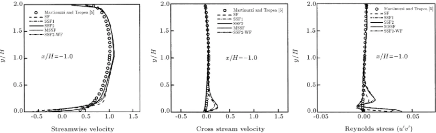
calculations are as follows: The inlet boundary con-dition was selected as a fully developed turbulent velocity distribution (one-seventh power law). It is noteworthy that this inlet boundary condition does not exactly correspond to that of the experiments. However, comparison of velocity prole and Reynolds stress at the upstream of the cube (x=H = 1:0)

shows negligible discrepancies with experiments for the SSF2 model, as observed in Figure 4. In other words, the dierence between the experimental inlet velocity prole and the one used in the present computations of the SSF2 model, diminishes upstream of the cube. The outlet boundary condition is of a convective type withU

c equal to the mean velocity, as follows: @u1

@t

+U c

@u1 @x1

= 0: (12)

Obviously, such a convective boundary condition is capable of predicting unsteady ow behavior at the exit with good accuracy. The spanwise boundary condition was selected as periodic. The minimum grid spacing used in the present computations is 0.03 in all three dimensions adjacent to the cube surface with a grid expansion ratio of 1.05. Using a no-slip boundary condition with such a grid resolution near the wall may raise the question of accuracy. To answer this question, the computations were performed with a wall function calculation [22]. The results showed a negligible dierence in predicted velocity components near the wall. The number of grid points used in the present computation was 11351100 in the x-, y- and z-direction, respectively. This was based

on the computations of Krajnovic and Davidson [10]. They used three dierent grid point distributions: 825066, 1626698 and 21066114 and

compared the mean reattachment lengths upstream

and downstream of the cube,X F and

X

R, respectively,

with the experiment. The percentage of error in 825066 grid points was 6.73 for X

F and 14.28

for X

R, which reduced to 5.77 and 9.75, respectively,

for 21066114 grid points. Such a decrease in error is

not economical when there is an increase of more than a million grid points, which increases computational time drastically. They also reported that very small dierences between the mean velocity proles were observed using the medium and ne grid. As both SF models and the one-equation model of Krajnovic and Davidson [10] are based on the spectral kinetic energy of turbulence, it seems that the same reasoning could be used for the present computations. The CFL (Courant-Friedrichs-Lewy) number is less than one for all computations with the maximum value of 0.95. The average time in the simulation was 200H=Umean, where H is the cube height andUmeanis the bulk velocity at

the inlet.

RESULTS

Results are presented in the form of time-averaged quantities, including streamline plots, velocity compo-nents, Reynolds stress and turbulent kinetic energy. The present computations were done for Re=40000, for which the experiments are available, namely, ow visualization studies and the detailed LDA measure-ments of Martinuzzi and Tropea [5]. They obtained the ow pictures given in Figures 2a and 3a, which show clearly the very complex nature of the ow in spite of its simple geometry. Figures 2 and 3 show the streamlines in the near channel oor and plane of symmetry, respectively, for dierent models used in the present calculations. All of them show a horseshoe vortex around the cube and the separation regions on the roof, lateral sides and behind the cube. The main point about horseshoe vortex is its converging-diverging behavior in the experimental measurement.

This phenomenon has not been observed in most of the previous computations (see Figures 2b, 2c and 2d), especially for Re = 40000 [9,10]. In the present work, such behavior was not predicted for most of the subgrid-scale models used except for the SSF2 model (see Figure 2h). Such behavior could be observed at a lower Reynolds number. Our computation for Re=3200 shows clearly this converging-diverging behavior of the horseshoe vortex (see Figure 2j).

The size and shape of the horseshoe vortex is clearly shown in Figure 2. As discussed by Martinuzzi and Tropea [5] (Figure 2a), two recirculation regions exist upstream of the cube. All calculations predicted the primary recirculation with its center located atX

R.

No author has detected the secondary recirculation zone, which is very small and close to the front side of cube, through numerical computation. In the lateral side of the cube, there are two saddle points, observed in the experiment (Figure 2a, points S1 and S2) and

separated by a distance. While most computations detected the pointS1, a limited number of them could

predict the point S2 (Figure 2c). In the present

computations, pointS2could be detected by the SSF2

model shown in Figure 2h. Computations obtained with other models in the present study could not show clearly the location of these points.

Figure 3 shows dierent recirculation zones at plane z = 0. Three recirculation zones are observed

clearly, both in the experiment and in the present com-putations. The most accurate results, concerning the downstream recirculation zone, are related to the SSF2 model computation that is observed in Figure 3e. The size and central location of the downstream recircula-tion zone obtained from SF, SSF1 and MSSF models have some dierences with the experiment. This may be due to the coarse grid resolution used in the present computations. Table 1 compares various lengths of sep-aration regions dened in Figure 1. It is observed that none of the models used can predict both upstream and

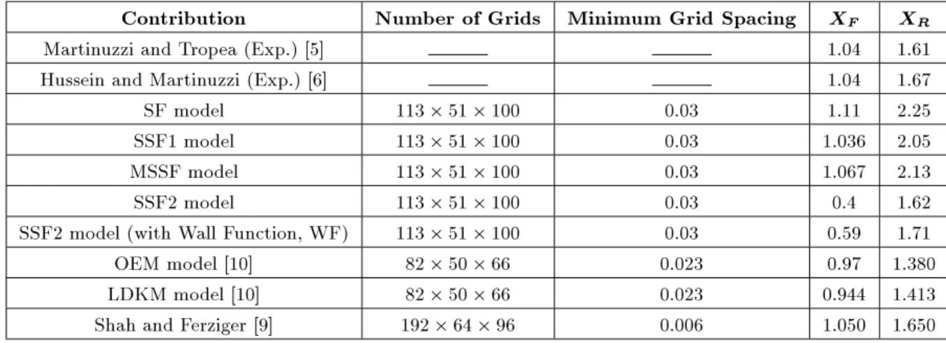
Table 1.

Reattachment lengths,X R and

X

F (Figure 1), obtained from models and experiment.

Contribution

Number of Grids Minimum Grid Spacing

XF XR

Martinuzzi and Tropea (Exp.) [5] 1.04 1.61

Hussein and Martinuzzi (Exp.) [6] 1.04 1.67

SF model 11351100 0.03 1.11 2.25

SSF1 model 11351100 0.03 1.036 2.05

MSSF model 11351100 0.03 1.067 2.13

SSF2 model 11351100 0.03 0.4 1.62

SSF2 model (with Wall Function, WF) 11351100 0.03 0.59 1.71

OEM model [10] 825066 0.023 0.97 1.380

LDKM model [10] 825066 0.023 0.944 1.413

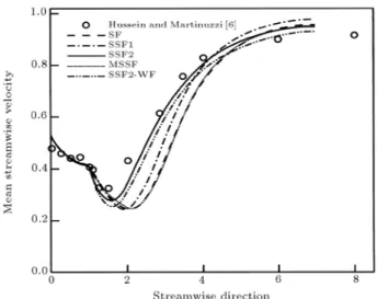
Figure 5.

Variation of time-averaged mean streamwise velocity at planez= 0.

downstream recirculation lengths correctly. The SSF2 model predicts downstream reattachment length in rea-sonable agreement with experimental data, except for the location of its center, but, its value, obtained for the upstream recirculation length, is too short. It should be mentioned that computations performed by SSF2 with a wall function could improve upstream recirculation length slightly. Other models predict the upstream recirculation length close to the experimental one, but, poor correspondence with experimental results were observed for the downstream recirculation length.

Mean streamwise velocity, integrated in a y

-direction at the plane z = 0, is plotted in Figure 5

for the various models used and compared with ex-perimental data. All computations follow the trend of experimental data. Among various models used in the present computations, SSF2 shows better agreement with the experiment, especially in the downstream recirculation region (1:5 < x < 4:0). The eect

of inserting a wall function in the SSF2 computation is observed in this gure, which shows a negligible decrease in mean streamwise velocity as compared to the SSF2 model.

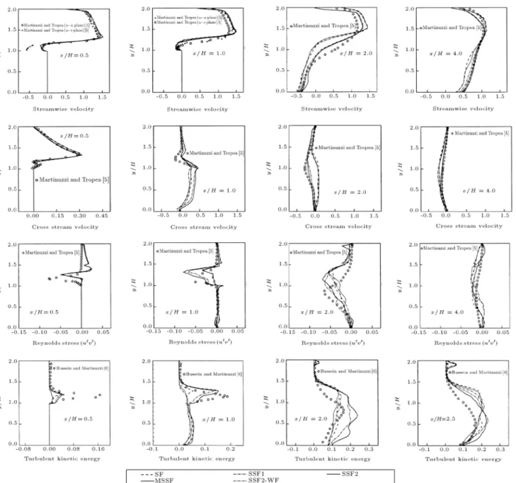
A series of time-averaged resolved velocities and turbulent stresses are computed and compared with the experiments in Figure 6. The locations are selected fromx=H= 0:5 to 4.0 atz= 0:0. Results obtained for

locations upstream of the cube were not shown, because no signicant ow feature exists in that region except for a small recirculation region. The computed mean velocity for this region showed good correspondence with the experiment, in spite of the dierences that exist in the upstream recirculation length computed, as mentioned in the preceding discussion. While streamwise velocity distribution near the top surface of the cube at x=H = 0:5 shows discrepancies with

the experimental data of u w plane measurements,

recirculation region above the cube, which, in turn, could be a result of low grid resolution and the QUICK scheme used for the discretization of convective terms. Among the four turbulence models used in the present computations, again, SSF2 shows better agreement with experimental data at x=H = 2:0. Figure 6, also,

shows the cross-stream velocity distribution. Shah and Ferziger [9] explained that the quality of computational results deteriorate for a vertical velocity component, as compared to the experimental data. Computations of Krajnovic and Davidson [10] showed considerable discrepancies in the vertical velocity component as compared to the experiment. As observed in Fig-ure 6, the authors' computations for a cross-stream velocity component show good correspondence with the experimental data, especially those obtained from the SSF2 model. Another parameter of interest in this ow is the Reynolds stresses. Prediction of the

u 0

v

0 prole reveals that all models predict the trend of

experimental results with some discrepancies, except at x=H = 1:0 for the SSF2 model. Displacement

of the predicted minimum value of u 0

v

0, as compared

to the experiment, is due to the dierent ow elds obtained, as mentioned before. As grid resolution and the discretization scheme is the same for all models, the question may arise as to why there are dierences in the predicted results. The reason for such behavior is the type of switching-o of the eddy viscosity in the three SSF models. As there is a continuous energy cascade from large to small eddies, the subgrid-scale model used should reveal this behavior. The MSSF and SSF1 mod-els, which use a cut-o function for removing turbulent eddy viscosity, produce acceptable results when a ne grid resolution is used. As a coarse-grid resolution was used in the present calculations, it is expected that these two models would not be able to produce acceptable results. The SSF2 model uses a continuous type of function for switching-o the turbulent eddy viscosity (see Equation 9) and, therefore, could perform better in a coarse grid resolution. So, results obtained from SSF2 are more reliable than those from SSF1 and MSSF.

Deciency in the predicted turbulent kinetic en-ergy variation over the cube is observed in Figure 6. Discrepancies reduce when moving toward the end point of the upper side of the cube. This is because of a smaller and thinner separation region as compared to the experiment, which implies that excessively large turbulent diusion should be created in this region. The prole of the computed turbulent kinetic energy forx=H = 2:0 and 2.5 follows the trend of the

exper-Figure 6.

Time-averaged streamwise, cross-stream, Reynolds stress and turbulent kinetic energy proles compared with experimental data at Re = 40000.

iment, with their values higher than the experimental ones. It is expected that less discrepancies occur between the present computation and the experiment for x=H > 2:5, but, no experimental data were

available for x=H > 2:5. Here, it is observed that

the SSF2 model is able to predict results closer to the experiment than other models, especially at the leading edge of the cube.

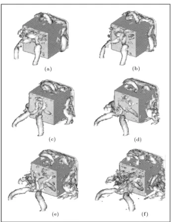
One of the complex phenomena in the ow over a cube in a channel is the formation of vortices and their subsequent stretching. Using vorticity isosurfaces for such phenomena is not suitable, as this method does not clearly distinguish the vortex near the cube. In order to identify the ow structures more clearly,

the technique of 5[23] was used in the present work. In this method, the vortex cores are obtained from instantaneous velocity elds. The vortex cores are iden-tied with a region of negative2, which is the second

largest eigenvalue of the tensor,S ik

S

k j + ikk j. The

denitions ofS

ijand ij, which are the symmetric and

anti-symmetric parts of the velocity gradient tensor (u

i;j= @u

i

@xj), are as follows: S

ij = ( u

i;j+ u

j;i)

=2; (13)

ij= ( u

i;j u

j;i)

=2: (14)

The isosurfaces of the second largest eigenvalue (2)

Figure 7.

Instantaneous isosurfaces of second invariant of the velocity gradientQ= 2500 with the time dierence between the two pictures oftUmean=H= 0:2 (view of the back face of the body (SSF2 model)).

the formation of a vortex in the top, side and back faces of the cube surface, along with its stretching and breakdown into small eddies.

CONCLUSION

Flow around a wall-mounted cube in a channel was computed using a Structure Function and three slightly varying versions of Selective Structure Function models at Re = 40000. A relatively coarse grid resolution with a minimum grid spacing of 0.03H was used in the present calculations. It was observed that, in general, the results obtained from Selective Structure Function modeling followed the trend of the experimental data better than those of the Structure Function. Among the three versions of the Selective Structure Function models used, the one with a smoothly varying func-tion (SSF2) was able to reproduce results in better agreement with the experiment than the others. This is due to the continuous type of the function used in switching-o the turbulent eddy viscosity, which performs better in a coarse grid resolution as compared with SSF1 and MSSF models. Modied Selective Structure Function modeling [20] could not predict better results than those of the SSF1 model for this geometry in such a coarse grid. Using a type of wall

C

k Kolmogorov constant E(K) kinetic energy spectrum G

x( x

i) lter function H cube height K

c cut-o wavenumber

P pressure

Re Reynolds number based on the height of the cube,UmeanH=

t time step

u

velocity vector

U

c convective mean velocity u

i instantaneous velocity components Umean average velocity at the entrance

x

position vector

x

i Cartesian coordinate,

x1;x2;x3

angle

kinematic viscosity v

SF

t turbulent eddy-viscosity obtained from

SF

minimum grid spacing

ij subgrid scale (SGS) stress tensor

x

i grid spacing

20 indicating function, Equation 8

REFERENCES

1. Castro, I.P. and Robins, A.G. \The ow around surface-mounted cube in uniform and turbulent streams",J. of Fluid Mech.,

79

(2), pp 307-335 (1977). 2. Castro, I.P.J. \Measurements in shear layers separat-ing from surface-mounted blu bodies", J. of Wind Eng. and Ind. Aerodynamics,

7

, pp 253-272 (1981). 3. Schoeld, W. and Logan, E. \Turbulent shear ow over

surface-mounted obstacles", ASME J. of Fluids Eng.,

112

, pp 376-385 (1990).

4. Larousse, A., Martinuzzi, R. and Tropea, C. \Flow around surface-mounted, three-dimensional obsta-cles",9th Int. Sym. on Turbulent Shear Flow, Springer-Verlag, pp 127-139 (1991).

5. Martinuzzi, R. and Tropea, C. \The ow around surface-mounted prismatic obstacles placed in a fully developed channel ow",ASME J. of Fluids Eng.,

115

, pp 85-92 (1993).

6. Hussein, H.J. and Martinuzzi, R.J. \Energy balance for turbulent ow around a surface mounted cube placed in a channel",Phys. of Fluids,

8

, pp 764-780 (1996).

7. Rodi, W., Ferziger, J.H., Breuer, M. and Pourquie, M. \Workshop on LES of ows past blu bodies", Rotach-Egern, Germany (June 1995).

8. Schmidt, S. and Thiele, F. \Comparison of numerical methods applied to the ow over wall-mounted cube",

Int. J. of Heat and Fluid Flows,

23

, pp 330-339 (2002). 9. Shah, K.B. and Ferziger, J.H. \A uid mechanicals view of wind engineering: Large eddy simulation of ow past a cubic obstacle",J. of Wind Eng. and Ind. Aerodynamics,

67

&

68

, pp 211-224 (1997).

10. Krajnovic, S. and Davidson, L. \Large eddy simulation of the ow around a blu body",AIAA Journal,

40

(5), pp 927-936 (2002).

11. Iaccarino, G., Ooi, A., Durbin, P.A. and Behnia, M. \Reynolds averaged simulation of unsteady separated ow",Int. J. Heat Fluid Flow,

24

, pp 147-156 (2003). 12. Rodi, W. \Comparison of LES and RANS calculations of the ow around blu bodies",J. of Wind Eng. and Ind. Aerodynamics,

69

, pp 55-75 (1997).

13. Krajnovic, S. and Davidson, L. \A mixed one-equation subgrid model for large-eddy simulation",Int. J. Heat Fluid Flow,

23

, pp 413-425 (2002).

14. Davidson, L. \Large eddy simulation: A dynamic one-equation subgrid model for three-dimensional Recircu-lating ow",11th Int. Symp. on Turbulent Shear Flow,

3

, pp 26.1-26.6 (1997).

15. Murakami, S. \Overview of turbulent models applied in CWE-1997",J. of Wind Eng. and Ind. Aerodynam-ics,

74-76

, pp 55-75 (1998).

16. Metais, O. and Lesieur, M. \Spectral large eddy sim-ulations of isotropic and stably-startied turbulence",

J. of Fluid Mech.,

239

, pp 157-194 (1992).

17. Lesieur, M. and Metais, O. \New trends in LES of turbulence",Ann. Rev. of Fluid Mech.,

28

, pp 45-82 (1996).

18. Suksangpanomrung, A., Djilali, N. and Moinat, P. \Large eddy simulation of separated ow over a blu rectangular plate",Int. J. of Heat and Fluid Flow,

21

, pp 655-663 (2000).

19. Rahnama, M. and Farhadi, M. \Large eddy simulation of ow over a wall-mounted cube", Proc. of 12th An-nual Conf. of Computational Fluid Dynamics, Ottawa, Canada, pp 708-714 (2004).

20. Ackermann, C. and Metais, O. \A modied selective structure function subgrid-scale model",J. of Turbu-lence,

2

, pp 011 (2001).

21. Suksangpanomrung, A. \Investigation of unsteady sep-arated ow and heat transfer using direct and large-eddy simulations", PhD Thesis, Department of Mech. Eng. University of Victoria, Victoria, USA (1999). 22. Mason, P.J. and Callen, N.S. \On the magnitude of the

subgrid-scale eddy coecient in large eddy simulations of turbulent channel ow",J. of Fluid Mech.,

162

, pp 439-462 (1986).

23. Jeong, J. and Hussein, F. \On the identication of a vortex",J. of Fluid. Mech.,

285

, pp 69-94 (1995).