Sharif University of Technology
Scientia IranicaTransactions A: Civil Engineering www.scientiairanica.com
A time varying optimal algorithm for active structural
response control
R. Mirzaei
a;and O. Bahar
ba. Department of Civil Engineering, Science and Research Branch, Islamic Azad University (IAU), Tehran, P.O. Box 14515-775, Iran.
b. Department of Structural Dynamics, International Institute of Earthquake Engineering and Seismology (IIEES), Tehran, P.O. Box 19395-3913, Iran.
Received 13 August 2013; received in revised form 7 December 2013; accepted 10 March 2014
KEYWORDS Time varying LQR; -method;
Time varying weighting matrix; Power consumption; Riccati equation.
Abstract.In this paper, a time varying optimal control algorithm (-method) is proposed to control building responses against environmental earthquake excitations. The proposed method is presented through dening a rational relation between the state variables of a structure with active and passive control systems with identical mechanisms. This procedure results in a time varying gain matrix with adaptable ability to external excitation, in order to decrease the extra need for maximum and/or total control force. Performance of the proposed method is examined by applying it to an eight-story shear type building subjected to various ground accelerations. Numerical results indicate that the proposed algorithm in some cases reduces the power consumption demand signicantly, without any reduction in control system performance, in comparison with the classical closed loop optimal control method, and, in the worst case, acts in a similar way.
© 2014 Sharif University of Technology. All rights reserved.
1. Introduction
Construction of tall buildings with enough strength against extraordinary loads, such as strong earthquakes and severe typhoons, besides their ability to deal with the resultant large deformations, has been the main concern of civil engineers for many years. Such struc-tures inherently have high exibility and low damping, so, it is important to suppress their responses not only for safety, but also for serviceability. Intensive research eorts have been devoted to balance these two eects, via the possibility of employing new protective systems in civil engineering. These include passive, semi-active, active, and hybrid control systems. Among them, ac-tive control systems are more attracac-tive than the others because of their ability to apply instant control forces, *. Corresponding author. Tel.: +98 411 6689251
E-mail addresses: [email protected] (R. Mirzaei); [email protected] (O. Bahar)
depending on the extent of the external disturbances and/or the state of the structural responses during vibrations. Active control has been studied extensively in engineering. Orlando and Goncalves [1] showed that the geometric nonlinearity of a pendulum absorber on the response of a tower can cause dynamic jumps and instability. In order to improve the eectiveness of the device, they implemented an active system based on position and velocity feedback. Mahato and Maiti [2] employed displacement and velocity feedback controllers to reduce the response of the composite laminate under hygrothermal conditions. Shisheie et al. [3] proposed a LQR approach to optimally tune the gains of a PI controller of rst order, plus time-delay systems. Sandoval et al. [4] evaluated the eectiveness of various alternative control devices (active, passive and semi-active) implemented as the link between two coupled buildings. Fitzgerald et al. [5] implemented active tuned mass dampers for the mitigation of in-plane vibrations in rotating wind turbine blades.
Venanzi et al. [6] proposed a method based on the genetic algorithm for optimized control of tall buildings with active mass dampers subjected to wind-induced vibrations.
Any active control system is included in an al-gorithm, which analyzes inputs and computes appro-priate control forces for imposition on the building. Until now, many active structural control algorithms have been proposed, each including many advantages and a few disadvantages. They are included as linear quadratic algorithms, pole placement, instantaneous optimal control, independent modal space control, and so on. The Linear Quadratic Regulator (LQR) is the most famous, which has been widely implemented in all elds of science, because of its simple procedure and ease of implementation on actual large scale systems. Among its three dierent branches: closed loop, open loop or closed-open loop algorithms, the classical closed loop control is the only feasible algorithm in structural control applications [7]. However, diculty in solving the Riccati matrix equation backward in time causes the excitation term to be ignored in order to acquire the desired control gains. Therefore, the classical closed loop control is approximately optimal and does not satisfy the optimality conditions entirely. To overcome this shortcoming, dierent algorithms have been pro-posed. Bahar et al. [8] proposed a new instantaneous control algorithm using the Wilson- method. Despite a suitable performance, however, the proposed algo-rithm, like other algorithms in this class, is sensitive to changes in time increment. Basu and Nagarajaiah [9] proposed a wavelet-based adaptive linear quadratic regulator formulation for the optimal control problem. Although no prior information on the excitation is required, stability criteria are not considered at all. Basu and Nagarajaiah [10] presented a method for the control of time varying systems based on wavelet transformation. By performing numerical examples, they showed that in cases where the conventional LQR failed to control the vibration response, the proposed controller eectively suppresses the instabilities in the linear time varying systems.
Changa et al. [11] proposed an active vibra-tion control technique for building structures using a learning-based lattice pattern controller under earth-quake excitations. Bagheri and Amini [12] proposed a procedure based on the pattern search method and the capability of wavelet analysis on uniform hazard earthquake accelerograms to acquire a more ecient control scheme than the LQR.
In this paper, a time varying closed-loop algo-rithm, based on the optimal theory, is proposed. It is assumed that the responses of active structures are a quotient of similar passively controlled structures, at any control time instant. This assumption results in a time-varying gain matrix. Since determined control
force may not always guarantee the stability of the building, the stability of the system is achieved by means of the Lyapunov stability criteria, which tends to a proper weighting matrix. By selecting an eight-story shear type building subjected to dierent ground accelerations, numerical examples are conducted to investigate and evaluate the eciency of the proposed procedure. The classical closed loop algorithm is used as a testimonial algorithm. Results show that the proposed method, in some cases, reduces signicantly the need for maximum and/or total control force consumption with a negligible drop in control system performance, and, in the worst case, acts in a similar manner.
2. Classical optimal linear quadratic closed loop regulator (CLLQR)
Consider a building equipped with an active control system excited by strong ground motion. The govern-ing dynamic equation of motion may be written in the following matrix form:
M x + C _x + Kx = MExg+ Du(t); (1)
where x is the n-dimensional displacement vector, and the dots state the derivative of x with respect to time, as the velocity and acceleration vectors; M, C and K are the n n mass, damping and stiness matrices of the structure, respectively; E is the n 1 inuence vector of the ground acceleration on the building masses; D is the n m location matrix of the control forces aecting the structure; and u(t) is the m 1 control force vector applied by the m actuators. With some manipulation, the equation of motion may be rewritten in terms of the state-space variables, Z, as follows:
_Z = AZ(t) + Bu(t) + Hf(t); Z(t0) = Z0; (2)
in which t0is the initial time instant, Z(t) is the vector
of state variables and A depicts the system matrix, respectively. Vector Z(t) and matrix A are dened as follows:
Z(t) = [x(t); _x(t)]T;
A =
0 I
M 1K M 1C
: (3)
In addition, matrix B and vector H are given as: B =
0 M 1D
; and H =
0
E
: (4)
In classical linear optimal control, a performance index, J(t), is dened in order to minimize building responses
and control forces to achieve the best structural per-formance, which is dened by:
J = Z tf
0
ZT(t)QZ(t) + uT(t)Ru(t)dt; (5)
where Q is a 2n 2n positive semi denite weighting matrix related to structural response, R is an r r positive denite weighting matrix related to active control force, and tf indicates the terminal time that
should be longer than the earthquake duration. To minimize the performance index, J, subjected to the constraint given by Eq. (2), the necessary conditions are as follows:
_ = AT(t) 2QZ(t); (6)
u(t) = 12R 1BT(t); (7)
in which, (t) is a 2n vector representing the Lagrange multiplier. The optimal control force vector, u(t), the Lagrange vector, (t), and the state vector, Z(t), can be solved using Eqs. (2)-(6) and Eq. (7). Notice that the control vector, u(t), in Eq. (7), is directly related to the Lagrange vector, (t). If the control force is assumed to be proportional to the state vector, Z(t), the LQR control is named an optimal closed-loop (CCLQR) control. In this case, one has:
(t) = P (t)Z(t); (8)
where P (t) is called the Riccati matrix and is achieved by solving the following nonlinear matrix equation:
_P(t)+P(t)A 12P (t)BR 1BTP (t)+ATP (T )+2QZ(t)
+ P (t)Hf(t) = 0; P (tf) = 0: (9)
There are two assumptions for Eq. (9) to be solved. First, the external disturbance, f(t), is equal to zero or is a white noise stochastic process. Second, the Riccati matrix is constant over the time [7]. Although, the second assumption is almost satised, the rst assumption is not fullled in almost all situations. In any case, Eq. (9) reduces to the following equation:
P A 12P BR 1BTP + ATP + 2Q = 0: (10)
By selecting appropriate Q and R weighting matrices, this equation is simply solved and, according to Eq. (7), the instant active control force is determined by the following relation:
u(t) = 12R 1BTP Z(t); (11)
in which, the constant control gain matrix is as follows:
G = 12R 1BTP: (12)
This procedure is simple, straightforward and strong. But, it seems that responses are not truly optimal because external disturbances are neglected in solving the matrix Riccati equation.
3. Time varying linear quadratic regulator-closed loop (-method)
Consider a structure enhanced by a passive control system in order to decrease its oor responses, due to environmental strong excitations such as typhoons or strong ground earthquakes. For such a structure, the governing equation of motion in terms of the state variables is as follows:
_Z(t) = A Z(t) + Hf(t); (13)
in which Z(t) denotes the state variables of the struc-ture equipped with passive control systems. Moreover, suppose this passive system is upgraded by installing an actuator to apply active control forces to obtain further reduction in responses. In this case, suppose, as a policy, the responses of the actively controlled structure, Z(t), are directly related to the responses of the passively controlled system, Z(t), as follows:
Z(t) = N(t)Z(t);
_Z(t) = _N(t)Z(t) + N(t) _Z(t); (14) where, N(t) is a proper transform matrix. It should be noticed that the transform matrix, N(t), is a magnier matrix, which relates the responses of the actively controlled system to the similar passively controlled system. Combining Eqs. (2)-(13) and Eq. (14) gives the following relation:
(AN N_ NA)Z(t) NBu(t)+(I N)Hf(t)=0: (15) Now, with regard to the constraint introduced in Eq. (15), and the quadratic performance index, J(t), i.e. Eq. (5), the corresponding Lagrangian, L, of the active optimal control problem can be written as follows:
L = Z tf
0
ZT(t)QZ(t) + uT(t)Ru(t)
+T(t)(AN _N NA)Z(t) NBu(t)+(I N)H
f(t)
dt:
(16) Consequently, the necessary conditions for optimal control become:
2ZT(t)Q + T(AN N_ NA) = 0;
2uT(t)R TNB = 0;
u(t) = 12R 1BTNT(t): (18)
Combining two last equations gives:
u(t) = R 1BTNT(AN N_ NA) TQZ(t): (19)
Selection of a proper transform matrix, N, at any mo-ment is a cumbersome and time consuming procedure. Therefore, after extensive analysis, a scalar matrix is proposed as an admissible N matrix by the following denition:
N(t) = (t)1 I; N(t) =_ 2_(t)(t)I; (20) where (t) is an admissible scalar function and I is the identity matrix with proper dimensions. Notice that, based on Eq. (14), the scalar function, (t), should be less than or equal to one, such that the condition of Z(t) Z(t) is satised. By inserting Eq. (20) into Eq. (19), the following expression for the control force is obtained:
u(t) = R 1(t)BTQZ(t); R(t) = _(t)
(t) !
:R: (21) It is seen that this trend directly aects the control force weighting matrix and, in turn, control forces are applied to the structure, in each time instant. Because of the appearance of (t) in the control force expression, the suggested control scheme is called the -method.
4. Stability criteria
In structural control, stability is an important issue, which must be carefully attended to. For linear time-invariant systems, the stability of a control system may be ensured by considering the location of the roots (eigenvalues) of the closed loop characteristic equation of the system matrix. These characteristic values are aected directly by the properties of the selected weighting matrices, as well as other properties of the building, such as mass, stiness and damping char-acteristics. Since, in the -method, the R weighting matrix is time dependent, selection of a proper stable Q weighting matrix needs more attention. In such situations, a convenient way to get a sucient stability margin and obtain proper performance is utilizing the second law of the Lyapunov stability theorem. Based on this theorem, a system is stable if a scalar Lyapunov function, V (Z) > 0 for Z 6= 0, V (Z) = 0 for Z = 0, and V (Z) ! 1 as Z ! 1, exists, such that its rst derivative, with respect to time, is negative denite for
all Z, i.e. _V < 0. To get a proper stability margin, we may consider a positive denite matrix, Q(t), such that the following denition is also a positive denite function:
V (t) = Z(t)TQ(t)Z(t) > 0; (22)
in which V (t) is a possible Lyapunov function. By taking the rst derivative of the Lyapunov function and considering Eqs. (2) and (21), the following expression is obtained:
_V =Z(t)T_Q(t) + Q(t)A + ATQ(t)
Q(t)BR(t) 1BTQ(t)Z(t): (23)
Based on the Lyapunov stability theorem, the weight-ing matrix, Q(t), will be a stable weightweight-ing matrix if the bracket in Eq. (23), which is very similar to a Riccati matrix equation, is a negative denite matrix. As a sucient condition, we may assume that the sum of all terms of the bracket in Eq. (23) is equal to a negative denite matrix, say -I0, where I0 is an
arbitrary positive denite matrix. Using this denition, we get:
_Q(t) + Q(t)A + ATQ(t) Q(t)BR(t) 1BTQ(t)
+ I0= 0: (24)
Now, if Eq. (24) is solved, for a dened I0 matrix and
a proper selected R(t) weighting matrix, the stable Q weighting matrix will be achieved. Extensive eorts show that the exact solution of Eq. (24) is computation-ally expensive, because it takes a long time to solve the equation in each time step. To overcome this diculty, by ignoring the derivative term of the Q weighting matrix, the approximate solution of Eq. (24) is here proposed. Performing such simplication, Eq. (24) becomes as follows:
Q(t)A + ATQ(t) Q(t)BR(t) 1BTQ(t) + I
0= 0:
(25) This simplication assumption will be examined in the following sections.
5. Evaluation criteria
To assess the eciency of the control algorithms, researchers have employed various indices, such as maximum displacement, velocity, acceleration of the stories, drift ratios of the adjacent oors and maximum base shear of the structures. Mirzaei and Bahar [13] have shown that, in general, performances of the family of optimal algorithms are so similar that their
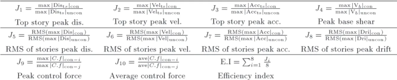
Table 1. Performance indices.
J1=max jDismax jDiststsjunconjcon J2=max jVelmax jVeltstsjunconjcon J3= max jAccmax jAcctstsjunconjcon J4=max jVmax jVbbjunconjcon
Top story peak dis. Top story peak vel. Top story peak acc. Peak base shear J5=RMS(max jDisjRMS(max jDisjunconcon)) J6=RMS(max jVeljRMS(max jVeljunconcon)) J7=RMS(max jAccjRMS(max jAccjunconcon)) J8=RMS(max jDrijRMS(max jDrijunconcon))
RMS of stories peak dis. RMS of stories peak vel. RMS of stories peak acc. RMS of stories peak drift J9= max jC:fjmax jC:fjcon jcon i J10= avejC:fjavejC:fjcon icon j E.I =P8i=1J8i
Peak control force Average control force Eciency index
Table 2. Characteristics of the strong ground motion acceleration records. Predominant
period (sec) PGA (g)
Strong ground motion duration
(sec)
Duration (sec) Earthquake
0.56 0.34 24.42 54 El-centro
0.34 0.82 0.36 48 Hyogo ken-Nanbu (Kobe)
0.36 0.171 31.90 50 Landers
0.38 0.357 4.47 30 Parkeld
dierences are negligible. Hence, in this paper, in order to have proper evaluation criteria for comparing the eciency of the control algorithms, other parameters are introduced. In this regard, two categories of criteria are tabulated in Table 1: (1) indices, J1 to J8, and,
also, E:I: index, which are related to the normalized reduction occurred in the structural responses, and (2) normalized indices, J9and J10, which are related to the
amount of the control force consumptions of dierent control systems.
Indices, J1 through J3, represent the criteria for
the maximum displacement, velocity, and acceleration responses of the top story, which are normalized to their corresponding uncontrolled values, i.e. the structure without any active or passive control systems. The performance index, J4, represents the normalized
maxi-mum base shear of the controlled building, with respect to the uncontrolled case. Indices, J5 though J8, show
the Root Mean Square (RMS) of the maximum story responses, such as displacement, velocity, acceleration and story drifts, with respect to the corresponding response quantity in the uncontrolled case. Finally, indices, J9 and J10, represent the maximum and
average amount of required control forces, with respect to the reference algorithm, which is a classical closed-loop optimal control algorithm. Meanwhile, an addi-tional parameter, called the eciency index (E:I:), is dened as the average of indices J1 thought J8. All
these indices help to give an overall insight into the performances of the various control systems.
6. Numerical example
A numerical example is carried out to evaluate the performance of the proposed method. Both
conven-tional LQR (CCLQR) and the proposed -method are used, separately, to control the extra seismic responses of an eight-story shear type building during dierent earthquake excitations. The properties of the building structure are as follows: mass, stiness and damping parameter of the oors are identical and their values are, respectively, equal to 345.5 tons, 3:404 105 kN/m, and 2937 tons-sec/m. The active control system includes an Active Mass Damper/Driver (AMD) system, which is installed on the roof. Its characteristics include a mass of about 29.63 tons, with a tuned frequency of about 98% of the rst vibration frequency of the building, and the damping about 25 tons-sec/m. In addition, the passive control system includes a Tuned Mass Damper (TMD) with similar dynamic specications on the roof of the building. Dynamics of the control systems are included in the dynamic equation of motion of the whole building. Hence, the interaction eects of the building and the control systems are considered.
The performance of the active controlled build-ing is considered durbuild-ing four dierent strong ground motions, which include the El Centro earthquake, the Hyogo ken-Nanbu (Kobe) earthquake, the Landers earthquake, and the Parkeld earthquake. Specica-tions of the acceleration records of these earthquakes are briey tabulated in Table 2.
6.1. Selection of proper scalar function (t) Mathematically, no restriction governs the selection of (t), unless its absolute value should be less than or equal to one, such that the condition of Z(t) Z(t) is satised. An exponential function can be a good candidate for this criterion, therefore, the general form is proposed as follows:
(t) = e g(t); (26)
in which the g(t) will be determined considering other requirements. In this regard, the term, _, in Eq. (21), is equal to _g(t). This term, multiplied by R, constructs R(t), which directly aects the magnitude of control forces. Since control forces applied during strong ground excitations are a function of earthquake time history, a suitable option for _g(t) may be as follows:
_g(t) = 1 + ea + e f(t)f(t); f(t) = Z t
0
xg
g
dtn; (27) where f(t) is an ascending function in the time do-main. With such selection, R(t) varies approximately uniform between two extent values, R
a and a+12R, during
the control time interval. For distinct values of a, analysis shows that the mentioned form does not tend to high eciency, the reason being that earthquake acceleration varies randomly and a uniform variation cannot account for this phenomenon. To eliminate this shortcoming, the terma 1
n _f(t)
is added to the dominator as the coecient of e f(t). Then, (t)
becomes: (t) = e
Rt
0
(
1+e f(t) a+(a (1n)f(t)_ )e f(t)
) dt
; f(t) =
Z t 0
xg
g
dtn; a 2 R+: (28)
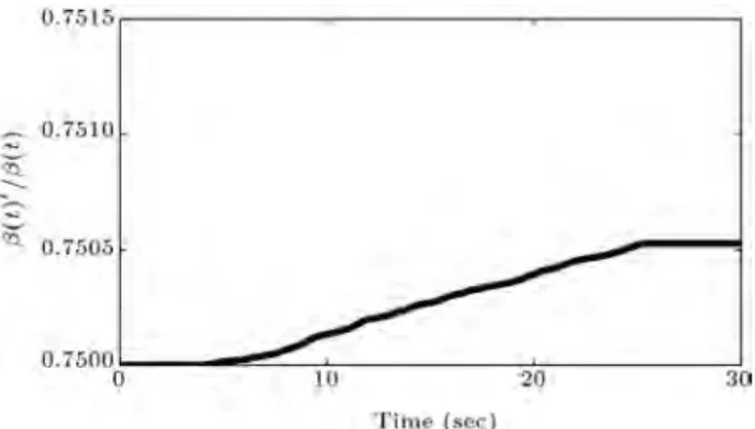
Using the El Centro earthquake excitation and imple-menting a trial and error procedure, appropriate values for variables a and n, in Eq. (28), are assigned equal to 8 and 1.5, respectively. The values were computed such that the responses of the controlled structures would decrease to the greatest possible extent. Using these values, variations of ( _=), which directly aect the instant values of control forces through Eq. (21), have been drawn during dierent ground accelerations in Figures 1-4.
In Figures 1 and 2, it is interesting that about 28 and 12 seconds after the starting control action,
Figure 1. Variation of ( _=) for El Centro ground excitation.
the need for inserting a control force is signicantly decreased, while, for instance, in Figure 4, by increasing control time duration, the need for active control forces is slightly increased. Generally, it is seen that using xed values for a and n, which are tuned for the best performance during the El Centro earthquake, leads to a proper performance during the other earthquakes. Also, variations of ( _=) are always less than unit value, meaning that the need for control forces during control time duration decreases.
6.2. Weighting matrices
In the control literature, a variety of Q and R weighting matrices, which are, respectively, pertinent to the state variables and control force, has been suggested.
Figure 2. Variation of ( _=) for Hyogo ken-Nanbu ground excitation.
Figure 3. Variation of ( _=) for Landers ground excitation.
Figure 4. Variation of ( _=) for Parleld ground excitation.
Commonly, Q and R matrices are determined in an oine manner, based on structural properties and known probable ground earthquakes. This perhaps causes a deciency in the control system during other unpredicted ground earthquakes. The proposed method is approximately exible, because only the I0
matrix should be chosen. Although the R matrix is also a predened value, its magnitude is continuously modied via the (t) function during each control time instant. In addition, since the Q matrix depends on I0 and R(t) matrices, it is not necessary to be
known beforehand. Hence, in the proposed method, the Q matrix is determined using the online solving of Eq. (24) or Eq. (25).
Mirzaei and Bahar [13] have shown that the sta-bility of the structures employing any optimal control method is guaranteed; in these structures, by using a positive semi denite weighting matrix, the matrix Riccati equation is solved.
In this study, the following arrangement of the Q weighting matrix, which is known as a proper matrix for the classical optimal algorithm, is also used for the positive denite matrix, I0:
Q = I0= 104
K 0
0 M
; (29)
where K and M are the matrices, with dimensionless numerical values corresponding to the stiness and mass matrices of the controlled building, omitting the stiness and mass values of the active mass damper/driver. The weighting matrix related to the control force, R, is assigned equal to 1.00 for all algorithms. Notice that matrix R is a scalar quantity, because only one AMD is installed at roof level.
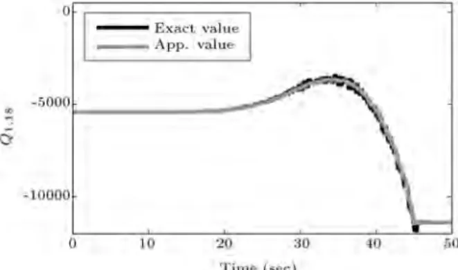
The proposed -method has great potential for use as an online procedure during the occurrence of earthquake excitations. Hence, in order to accelerate determination of the instantaneous Q matrix in each time instant, changes of some elements of Q(t) acquired from exact solution, Eq. (24), and from approximate solution, Eq. (25), are compared together in Fig-ures 5-8, during El Centro and Landers earthquakes. Results show that, although the elements of the Q matrix are rapidly changed with time, its estimation is good enough, especially its determination, which is much faster than the exact solution. The Figures obviously show that the approximate solution can accurately determine the values of the Q matrix. So, the major contribution of the approximate solution is acquired, which will be ease of implementation of the proposed time varying scheme, while accuracy is preserved. Naturally, this encourages one to take advantage of these benets, and, therefore, the ap-proximate solution will be utilized in the numerical investigations.
Figure 5. Variation of Q1;1 element for exact and
approximate solutions; El Centro earthquake.
Figure 6. Variation of Q1;18 element for exact and
approximate solutions; El Centro earthquake.
Figure 7. Variation of Q1;1 element for exact and
approximate solutions; Landers earthquake.
Figure 8. Variation of Q1;18 element for exact and
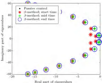
Figure 9. Stability diagram of the controlled building during El Centro earthquake.
Figure 10. Stability diagram of the controlled building during Hyogo ken-Nanbu earthquake.
6.3. Investigation of stability
Satisfaction of the stability criteria is the most im-portant problem in active structural control problems. Since the new proposed method results in a time-varying gain matrix, the stability diagram of the whole controlled building may be changed during each time instant. To prevent the occurrence of instability of the structure, stability diagrams of the building during dierent ground earthquakes are presented in Figures 9-12. The results are compared with the stability diagram of the building when it is passively controlled.
Stability diagrams show that the controlled build-ing is stable in all cases. But, the stability margin of the controlled building during the control time for dierent earthquakes may signicantly alter (Figures 9-12). For instance, by increasing control time, the stability margin of the controlled building during El
Figure 11. Stability diagram of the controlled building during Landers earthquake.
Figure 12. Stability diagram of the controlled building during Parleld earthquake.
Centro and Hyogo ken-Nanbu (Kobe) earthquakes has a tendency towards the stability margin of the passive control system. It means that the active control system, after passing the strong part of the earthquake, performs like an equivalent passive system. This may signicantly decrease required control forces. On the other hand, during Landers or Parkeld earthquakes, the performance of the control system does not change. In other words, the control system actively works all the time, expecting no reduction observed in the control forces.
6.4. Results and discussion
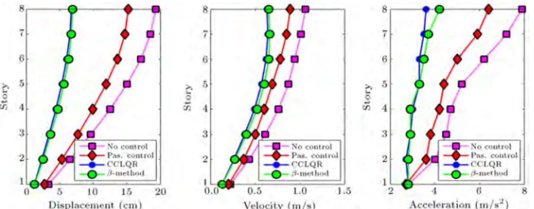
Responses of a controlled building using the new -method under four dierent earthquakes, El Centro, Hyogo ken-Nanbu (Kobe), Landers and Parkeld, are determined and depicted in Figures 13-16. Results include the maximum displacement, velocity, and
ac-Figure 13. The maximum responses of the building oors due to El Centro earthquake.
Figure 14. The maximum responses of the building oors due to Hyogo ken-Nanbu earthquake.
Figure 15. The maximum responses of the building oors due to Landers earthquake.
Table 3. Performance indices for building, subjected to El Centro, Hyogo ken-Nanbu (Kobe), Landers and Parkeld earthquakes.
El Cento Kobe Landers Parkeld
Index P
assiv
e
con
trol
CCLQR
-metho
d
P
assiv
e
con
trol
CCLQR
-metho
d
P
assiv
e
con
trol
CCLQR
-metho
d
P
assiv
e
con
trol
CCLQR
-metho
d
J1 0.79 0.35 0.36 0.94 0.50 0.53 0.78 0.34 0.35 0.89 0.35 0.38
J2 0.84 0.59 0.61 0.96 0.60 0.63 0.78 0.44 0.45 0.95 0.60 0.62
J3 0.81 0.46 0.53 0.96 0.55 0.63 0.97 0.65 0.74 0.93 0.50 0.55
J4 0.83 0.37 0.38 0.94 0.51 0.55 0.74 0.34 0.35 0.85 0.47 0.48
J5 0.79 0.35 0.37 0.94 0.51 0.54 0.77 0.33 0.35 0.88 0.40 0.41
J6 0.83 0.63 0.66 0.96 0.61 0.64 0.85 0.51 0.52 0.92 0.62 0.62
J7 0.84 0.57 0.59 0.95 0.73 0.76 0.89 0.66 0.68 0.95 0.64 0.66
J8 0.80 0.37 0.38 0.94 0.54 0.56 0.78 0.37 0.38 0.89 0.48 0.49
E.I - 0.46 0.49 - 0.57 0.61 - 0.45 0.48 - 0.51 0.53
J9 - 1 0.93 - 1 1.03 - 1 0.92 - 1 0.90
J10 - 1 0.72 - 1 0.62 - 1 0.99 - 1 1.06
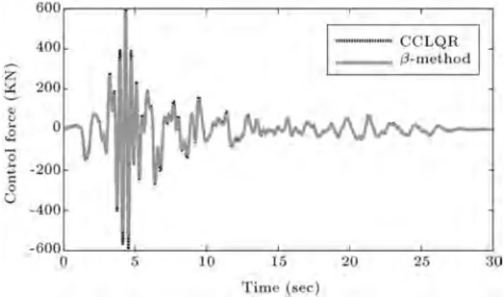
Figure 17. Active control force during El Centro earthquake.
celeration responses of the oors obtained from three cases: without control action, and with passive and active control systems. For the active control system, two algorithms are also used that are the conventional LQR (CCLQR) and the proposed time varying scheme, -method.
The corresponding control force time histories for all cases are compared in Figures 17-20 for all earthquakes. Moreover, in order to provide more realistic insight into the performance of both methods, calculated indices are tabulated in Table 3.
Comparing results apparently show that all the controlled responses obtained by the use of two dif-ferent control algorithms are very similar during var-ious earthquake excitations. There is only a small dierence between the acceleration responses of the above oors. For instance, the maximum dierence at roof level during the El Centro earthquake is about 7% in which the -method presents slightly greater values, with respect to CCLQR. It is interesting that
Figure 18. Active control force during Hyogo ken-Nanbu (Kobe) earthquake.
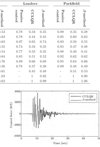
Figure 19. Active control force during Landers earthquake.
based on the results tabulated in Table 3, the need for peak and average control force requirements for this case are reduced by 7% and 28%, respectively (Figure 17). This indicates that the total energy demands for the proposed new control scheme are
Figure 20. Active control force during Parleld earthquake.
signicantly decreased. Considering the results for the Hyogo ken-Nanbu (Kobe) earthquake, it shows that, although the peak control force is increased about 3%, the reduction in the average control force is almost 38% (Figure 18). For the two other earthquakes, i.e. Landers and Parkeld, the required maximum control forces are decreased about 10%, while the other results are almost similar.
It is mentioned that in some cases, like Hyogoken-Nanbu (Kobe) or Parkeld earthquakes, it seems that the passive control system is not working correctly to alleviate the extra responses of the building. This is because the passive control system is not designed separately, but the same mechanism of the designed active control system, without inserting control force to the building, is used as a passive system. It is clear that by better tuning the characteristics of the passive system against these mentioned earthquakes, better results will be obtained.
Briey, the results show that the proposed time varying controller has the inherent capability and exi-bility to account for the variaexi-bility in the nature of the response, using a predened scalar function related to the variations of ground acceleration. The performance of the proposed controller is better, in terms of reducing the need for energy power, in some cases, compared to the classical LQR controller. And, in the worst case, it approximately needs a similar amount of energy, as in the case of an LQR controller. Moreover, the proposed method, in some cases, may alleviate the need for maximum control force consumption, with a negligible drop in reduced controlled responses, in comparison with the CCLQR scheme.
7. Conclusions
In this paper, a new active control method, named the -method, through dening a rational relation between the state variables of a structure with two active and passive control systems with identical mechanisms, is proposed. Using a scalar function, which is dened
as an external excitation dependent function, the -method presents a time varying adaptive control gain. Using the Lyaponuv stability criteria, proper weighting matrices for ensuring the entire stability of the whole building are guaranteed. Using the new proposed method, the performance of an actively controlled eight-story shear type building, in comparison to the classical optimal control method, shows that: (1) the performance of the new method with negligible dierences is very similar to that of the classical method, and (2) in some cases, without decreasing performance, maximum and/or average control forces are much decreased. Overall, in spite of signicant power saving, in some cases, a slight drop occurs in performance, which may be observed as the inherent exibility of the proposed method to reduce energy demand. This makes it an attractive time varying control method for seismic vibration control of struc-tures.
References
1. Orlando, D. and Goncalves, P.B. \Hybrid nonlinear control of a tall tower with a pendulum absorber", Struct. Eng. Mech., 46(2), pp. 153-177 (2013). 2. Mahato, P.K. and Maiti, D.K. \Active vibration
con-trol of smart composite structures in hygrothermal environment", Struct. Eng. Mech., 44(2), pp. 127-138 (2012).
3. Shisheie, R., Shaeenejad, I., Moallemi, N. and Nov-inzadeh, A.B. \Linear quadratic regulator time-delay controller for hydraulic actuator", J. Basic. Appl. Sci. Res., 2(3), pp. 2607-2618 (2012).
4. Sandoval, M.E., Ugarte, L.B. and Spencer, B.F. \Study of structural control in coupled buildings", Proceeding of the15th World Conference on Earthquake Engineering, Lisbon, Portugal, September (2012). 5. Fitzgerald, B., Basu, B. and Nielsen, S.R.K. \Active
tuned mass dampers for control of in-plane vibrations of wind turbine blades", Struct. Contr. Health Monit., 20(12), pp. 1377-1396 (2013).
6. Venanzi, I., Ubertini, F. and Materazzi, A.L. \Optimal design of an array of active tuned mass dampers for wind-exposed high-rise buildings", Struct. Contr. Health Monit., 20(6), pp. 903-917 (2013).
7. Soong, T.T., Active Structural Control: Theory and Practice, John Wiley & Sons, Inc., New York, N.Y. 10158 (1990).
8. Bahar, O., Banan, M.R., Mahzoon, M. and Kitagawa, Y. \Instantaneous optimal wilson- control method", Eng. Mech- ASCE, 129(11), pp. 1268-1276 (2003). 9. Basu, B. and Nagarajaiah, S. \A wavelet-based
time-varying adaptive LQR algorithm for structural con-trol", Eng. Struct., 30(9), pp. 2470-2477 (2008). 10. Basu, B. and Nagarajaiah, S. \Multi scale
wavelet-LQR controller for linear lime varying systems", J. Eng. Mech., 136(9), pp. 1143-1151 (2010).
11. Changa, S., Kimb, D., Kimc, D.H. and Kangd, K.W. \Earthquake response reduction of building structures using learning-based lattice pattern active controller", J. Earthquake. Eng., 16(3), pp. 317-328 (2012). 12. Bagheri, A. and Amini, F. \Control of structures
un-der uniform hazard earthquake excitation via wavelet analysis and pattern search method", Struct. Contr. Health Monit., 20(5), pp. 671-685 (2013).
13. Mirzaei, R. and Bahar, O. \A new view on optimal control algorithms", JSEE, 13(3), pp. 177-129 (2011).
Biographies
Rahman Mirzaei received his BS degree from Tabriz University, Iran, and his MS degree in Structural Engi-neering from Iran University of Science and Technology,
Iran, in 2004 and 2006, respectively. He is currently a PhD degree candidate in Structural Engineering at the Science and Research Branch of the Islamic Azad University, Tehran, Iran. His professional interests focus on structural dynamics, especially structural response control.
Omid Bahar earned his PhD degree in Structural Engineering from Shiraz University, Shiraz, Iran. He spent a short time as visiting scholar in Professor Kita-gawa's Laboratory at Hiroshima University, Japan, during his PhD research, working on the performance of active structural control during strong ground mo-tion. He is currently faculty member of the Interna-tional Institute of Earthquake Engineering and Seis-mology (IIEES), Tehran, Iran. Dr. Bahar's research interests include innovations in structural control and new methods in system identication and structural damage detection.