ISSN: 2322-1666 print/2251-8436 online
REPRODUCING KERNEL METHOD FOR SOLVING WIENER-HOPF EQUATIONS OF THE SECOND KIND
A. ALVANDI, T. LOTFI AND M. PARIPOUR
Abstract. This paper proposed a reproducing kernel method for solving Wiener-Hopf equations of the second kind. In order to elim-inate the singularity of the equation, a transform is used. The advantage of this numerical method is the representation of exact solution in reproducing kernel Hilbert space and accuracy in numer-ical computation is higher. On the other hand, by improving the traditional reproducing kernel method and the definition of the op-erator of W Hilbert space, the solutions of Wiener-Hopf equation of the second kind are obtained. The approximate solution converges uniformly and rapidly to the exact solution. Numerical examples indicate that this method is efficient for solving these equations. The validity of the method is illustrated with two examples.
Key Words: Reproducing kernel method, Wiener-Hopf equation, Singular integral equa-tion..
2010 Mathematics Subject Classification:13A15, 13F30, 13G05.
1. Introduction
In recent years, numerical methods for solving singular integral equa-tions have attracted a lot of attention. These equaequa-tions have many ap-plications in mathematics and engineering, see for instance Hunter [1], Paget [2], Lu [3], Krenk [4], Pedas [5]. Recently, the reproducing ker-nel method for solving singular integral equations in reproducing kerker-nel space is developed. The advantage of this method is that it converges Received: 25 January 2016, Accepted: 23 May 2016. Communicated by Mohammad Zareb-nia;
∗Address correspondence to Mahmoud Paripour; E-mail: [email protected] c
⃝2016 University of Mohaghegh Ardabili. 56
uniformly and rapidly to the exact solution. See Jin [6], Du [7], Chen [8], Shen [9]. The Wiener-Hopf equation of the second kind is of the form
(1.1) y(t) +
∫ ∞
0
k(t−s)y(s)ds=g(t), 0≤t <∞,
wherek(t)∈L1(R) andg(t)∈Lp[0,∞)(1≤p <∞) are given functions.
Many authors considered methods for solving equation (1.1) includ-ing the Clenshaw-Curtis quadrature method, Clenshaw-Curtis-Rational method and so on [10,11,12,13,14]. In this study, a new method of solv-ing solution is proposed in a reproducsolv-ing kernel Hilbert space(RKHS). It is called reproducing kernel method. The rest of the paper is orga-nized as follows. In section next, the reproducing kernel Hilbert space for solving (1.1) is introduced. In section 3, we discuss reproducing kernel method for (1.1). We transform (1.1) into integral equation of finite interval by substituting the variables t and sby t = α(11+−ττ), and s= α(11+−zz) respectively:
Y(t) + 2α
∫ 1
−1
K(τ, z)
(z+ 1)2 Y(z)dz =G(τ), −1< τ <1.
We will show thatK(τ, z) has singularities alongτ =z when τ tend to -1, to eliminate the singularities, we introduce a new function X(z) ≜
Y(z)
(z+ 1)2. We then proof the numerical method is stable and conver-gent. Section 4 illustrates two numerical examples. It is shown that the reproducing kernel method proposed in this paper is efficient. Finally, concluding remarks are given in Section 5.
2. Preliminaries
2.1. A reproducing kernel Hilbert spaceWm[−1,1]. In the section, a RKHS Wm[−1,1] is introduced for solving Eq. (1.1). The representa-tion of reproducing kernel becomes simple by improving the definirepresenta-tion of traditional inner product see [15,16,17,18,19], inWm[−1,1].
Definition 1.2.1. Wm[−1,1] ={u(x)|u(m−1)(x) is an absolutely con-tinuous real value function,u(m)(x)∈L2[−1,1]}.The inner product and norm in Wm[−1,1] are given respectively by
(2.1) ⟨u, v⟩=
m∑−1
i=0
u(i)(−1)v(i)(−1) +
∫ 1
−1
and
(2.2) ∥u∥m=
√
⟨u, u⟩m, u, v∈Wm[−1,1].
Wm[−1,1] is a reproducing kernel space and its reproducing kernelRx(y)
can be obtained. Now let us find out the expression form of the repro-ducing kernel functionRx(y) in W2[−1,1].
⟨u(y), Rx(y)⟩=u(−1)Rx(−1) +u′(−1)R′x(−1) + ∫ 1
−1
u′′(x)R′′x(y)dy
=u(−1)Rx(−1) +u′(−1)Rx′(−1) +u′(y)R′′x(y)|1−1−
u(y)R′′′x(y)|1−1+
∫ 1
−1
u(y)R(4)x (y)dy.
Not that the definition of the reproducing kernel u(x) = ⟨u(y), Rx(y)⟩
inWm[−1,1], the following equalities are necessary.
(2.3) Rx(4)(y) =δ(y−x)
(2.4) Rx(−1) +R′′′(−1)= 0, (2.5) R′x(−1)−R′′x(−1) = 0, (2.6) R′′′x(1) = 0, R′′x(1) = 0.
From (2.3), it has R(4)x (y) = 0 as y ̸= x. λ4 = 0 is its characteristic
equation. Then the representation of the reproducing kernel is assumed by
(2.7) Rx(y) =
{∑4
i=1ciyi−1, y≤x,
∑4
i=1diyi−1, y > x,
where coefficientsci, di,{i= 1,2,3,4},could be obtained by solving the
(2.8)
Rx(m)(x+ 0) =Rx(m)(x−0), (m= 0,1,2),
Rx′′′(x+ 0)−R′′′x(x−0) = 1, Rx(−1) +R′′′x(−1) = 0,
Rx′(−1)−R′′x(−1) = 0, Rx′′′(1) = 0,
Rx′′(1) = 0.
3. Solving Eq. (1.1) in the Reproducing Kernel Space
3.1. An identical transformation of equation (1.1).
In this section, we proposed an identical transformation of equation (1.1):
y(t) +
∫ ∞
0
k(t−s)y(s)ds=g(t), 0≤t <∞.
We assume that k(t) ∈L1(R) is semi-smooth, i.e., k(t)∈Cr(0,∞) and k(t) ∈ Cr(−∞,0) for certain positive integer r and y(t) ∈ Cr(0,∞) satisfying
(3.1) |y(t)| ≤ c
t2
for certainc > 0 for larget. Substituting the variables t and sin (1.1)
α(1−τ) 1+τ ,and
α(1−z)
1+z respectively, we get the following integral equation
(3.2) Y(τ) + 2α
∫ 1
−1
K(τ, z)
(z+ 1)2 Y(z)dz=G(τ), −1< τ ≤1, where
K(τ, z) =k
(
α(1−τ) 1 +τ −
α(1−z) 1 +z
)
, Y(τ) =y
(
α(1−τ) 1 +τ
)
,(3.3) G(τ) =g
( α(1−z)
1+z )
.
We notice that the kernel function of (3.2) has singularities alongz=τ asτ tend to−1 since the denominatorsτ+ 1, z+ 1 and (z+ 1)2 tend to infinity. On the other hand, under the assumption (3.1), the integral of (3.2) satisfies
|K(τ, z)
(z+ 1)2Y(z)|=|
K(τ, z) (z+ 1)2y(
α(1−z) z+ 1 )| ≤ |
K(τ, z) (z+ 1)2c(
α(1−z) (z+ 1) )
=|αcK2(1(−τ,zz))2|,
i.e., |K(z+1)(τ,z2)Y(z)|is bounded. Now we proposed a way to eliminate the
singularities. Since the factor 1
(z+ 1)2 in the kernel function of (3.2) is independent ofτ, we define a new function X(z) ≜ Y(z)
(z+ 1)2 and then subtract the singularities by reformulating (3.2) as
(3.4)
(τ+ 1)2X(τ) + 2α
∫ 1
−1
K(τ, z)X(τ)dz+ 2α
∫ 1
−1
K(τ, z)(X(z)−X(τ))dz =G(τ).
3.2. Representation of Exact Solution for Wiener-Hopf Equa-tions of the Second Kind.
In this section, exact solution of Eq. (1.1) is obtained by defining op-eratorL:W2[−1,1]−→L2[−1,1],then Equation (3.4) can be converted into the form as follows :
(3.5) (Lu)(τ) =G(τ), −1< τ ≤1,
(3.6)
(Lu)(τ) = ((τ+ 1)2+ 2α
∫ 1
−1
K(τ, z)dz)u(τ) + 2α
∫ 1
−1
K(τ, z)(u(z)−u(τ))dz,
it is easy to prove L is a bounded linear operator, and let L∗ is the conjugate operator of L. In order to obtain the representation of the exact solution of Eq. (1.1), let
φi(x) =Rxi(x), ψi(x) =L∗φi(x) = [LyRx(y)](xi), (i= 1,2, . . .), where{xi}∞i=1 is dense in the interval [−1,1].Hence, one gets
(3.7) ψi(x) = ((xi+ 1)2+ 2α ∫ 1
−1
K(xi, y)dy)R(xi, x)
+2α∫−11K(xi, y)(R(x, y)−R(xi, y)dy.
Theorem 3.1.If{xi}∞i=1 is dense in [−1,1],then{ψi(x)}∞i=1 is complete inW2[−1,1].
Proof. If for any u(x) ∈ W2[−1,1], it has ⟨u(x), ψi(x)⟩ = 0 i =
namely
⟨u(x), ψi(x)⟩=⟨u(x),(LyRx(y)(xi)⟩
=Ly⟨u(x), Rx(y)⟩(xi)
= [Lyu(y)](xi) = 0.
(3.8)
Note that {xi}∞i=1 is a dense set. It follows that Lyu(x)≡0.From the existence and uniqueness of the solution of Eq. (1.1), it follows that u(x)≡0. So {ψi(x)}i∞=1 is complete in W2[−1,1]. □
By Gram-Schmidt process, we obtain an orthogonal basis {ψ¯i(x)}∞i=1 of W2[−1,1],such that
(3.9) ψ¯i(x) =
i ∑ k=1
βikψk(x),
whereβik are orthogonal coefficients. In order to obtain βik, let
ψi(x) = i ∑ k=1
Bikψ¯k(x).
⟨ψi(x),ψ¯i(x)⟩= i−1
∑ k=1
Bik2 +B2ii,
Bii= v u u
t⟨ψi(x), ψi(x)⟩ −∑i−1 k=1
B2ik.
βii=
1
√
⟨ψi(x), ψi(x)⟩ − ∑i−1
k=1Bik2
.
(3.10) βij =βii
−∑i−1
k=j
Bikβkj .
Theorem 3.2. Ifu(x) is the solution of Eq. (1.1), then
(3.11) u(x) =
∞
∑ i=1
i ∑ k=1
Proof. u(x) can be expanded to Fourier series in term of normal orthog-onal basis ¯ψi(x) in W2[−1,1],
u(x) =
∞
∑ i=1
⟨u(x),ψ¯i(x)⟩ψ¯i(x) =
∞ ∑ i=1 i ∑ k=1
βik⟨u(x), ψk(x)⟩ψ¯i(x)
= ∞ ∑ i=1 i ∑ k=1
βik⟨u(x),L∗φk(x)⟩ψ¯i(x) =
∞ ∑ i=1 i ∑ k=1
βik⟨Lu(x), φk(x)⟩ψ¯i(x)
= ∞ ∑ i=1 i ∑ k=1
βik⟨G(x), φk(x)⟩ψ¯i(x) =
∞ ∑ i=1 i ∑ k=1
βikG(xk) ¯ψi(x).
(3.12)
The proof is complete.□
By truncating the series of the left-hand side of (3.11), we obtain the approximate solution of Eq. (1.1)
(3.13) un(x) =
n ∑ i=1 i ∑ k=1
βikG(xk) ¯ψi(x).
un(x) in (3.13) is the n-term intercept of u(x) in (3.11), so un(x) −→
u(x) in W2[−1,1] asn−→ ∞.
Theorem 3.3. Suppose the following conditions are satisfied (i)∥un(x)∥W2 is bounded;
(ii){xi}∞i=1 is dense in [−1,1].Thenn-term approximate solutionun(x)
converges to the exact solutionu(x) of Eq. (1.1) and the exact solution is expressed as
(3.14) u(x) =
∞
∑ i=1
Biψ¯i(x),
whereBi = ∑i
k=1βikG(xk).
Proof. (i) The convergence of un(x) will be proved. From (3.13), one
gets
(3.15) un(x) =un−1(x) +Bnψ¯n(x).
From the orthogonality of{ψ¯i(x)}∞i=1,it follows that ∥un(x)∥2W2 =∥un−1(x)∥2W2 +∥Bn∥2.
The sequence ∥un(x)∥W2 is monotone increasing. Due to ∥un(x)∥W2
there exists a constant csuch that (3.16)
∞
∑ i=1
Bi2 =c.
letm > n, in view of (um−um−1)⊥(um−1−um−2)⊥ · · · ⊥(un+1−un),
it follows that
∥(um−un)∥2W2 =∥um−um−1+um−1−um−2+· · ·+un+1−un∥2W2
=∥um−um−1∥2W2 +∥um−1−um−2∥2W2 +. . .
(3.17)
+∥un+1−un∥2W2 = m ∑ i=n+1
(Bi)2 −→0,(n−→ ∞).
Considering the completeness ofW2[−1,1], it has un(x)
∥.∥W2
−→ u(x), n−→ ∞. (ii) It is proved thatu(x) is the solution of Eq. (3.5). From (3.14), it follows
(Lu)(xj) =
∞
∑ i=1
Bi⟨Lψ¯i(x), φj(x)⟩
=
∞
∑ i=1
Bi⟨ψ¯i(x),L∗φj(x)⟩
=
∞
∑ i=1
Bi⟨ψ¯i(x), ψj(x)⟩,
it follows that
n ∑
i=1
βnj(Lu)(xj) =
∞
∑ i=1
Bi ⟨¯
ψi(x), n ∑ j=1
βnjψj(x) ⟩
W2
=
∞
∑ i=1
Bi⟨ψ¯i(x),ψ¯n(x)⟩W2 =Bn.
Ifn= 1, then (Lu)(x1) =G(x1). Ifn= 2 thenβ21(Lu)(x1)+β22(Lu)(x2) = β21G(x1) +β22G(x2). It is clear that (Lu)(x2) = G(x2). Moreover,
it is easy to see by induction that (Lu)(xj) = G(xj). Since {xi}∞i=1 is dense on [−1,1],for anyx∈[−1,1]
(3.18) (Lu)(x) =G(x).
That is,u(x) is the solution of Equation (3.5) and
(3.19) u(x) =
∞
∑ i=1
Biψ¯i(x).
The proof is complete. □
3.3. The Stability of the Solution on the Eq. (3.5).
Letu(x) be a solution of (3.5). It is called that the approximate method on solutionu(x) from un(x) with the right-hand side Gn(x) is stable in
W2[−1,1],if limn→∞∥G−Gn∥W2 = 0, then limn→∞∥u−un∥W2 = 0.
Let (Lun)(x) =Gn(x) and G(x) =Gn(x) +ϵn(x),
where ϵn(x) is a perturbation and ϵn(x) → 0(n → ∞). See [20, 21].
From the form (3.11), note that
u(x) =
∞
∑ i=1
i ∑ k=1
βikG(xk) ¯ψi(x),
and
un(x) =
∞
∑ i=1
i ∑ k=1
βikGn(xk) ¯ψi(x),
it follows
u(x)−un(x) =
∞
∑ i=1
i ∑ k=1
βikϵn(xk) ¯ψi(x) =L−1ϵn(x).
From the continuity ofL−1 and ϵn(x)→0(n→ ∞),it follows
lim
n→∞∥u(x)−un(x)∥=∥L
−1∥ lim
n→∞|ϵn(x)|= 0.
Then, the method is stable.
4. Numerical examples
Example 4.1. Consider u(t) +∫0∞ 1
1 + (t−s)2 u(s)ds=g(t), 0≤t <∞, where
g(t) = 1 1 +t2 +
1
4 +t2(π+arctan(t)) +
ln(1 +t2) t(4 +t2) .
The exact solution of the equation isu(t) = 1
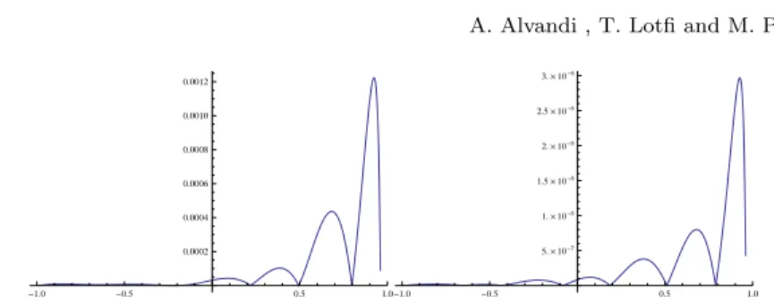
(1 +t2).Using the method presented in section 3, taking n= 11 and n= 20. The absolute errors u11−u and u20−u are given in Table 1 and Figure1.
Table 1
Numerical results of Example 4.1 Node |u11−u| |u20−u|
-0.9 8.77083E-6 1.54070E-8
-0.7 5.11982E-6 9.70029E-9
-0.5 6.89540E-6 1.41000E-8
-0.3 2.08658E-6 5.96931E-8
-0.1 9.13911E-6 1.90117E-8
0.1 4.23227E-5 1.11963E-7
0.3 6.43560E-5 2.80711E-7
0.5 1.41120E-5 5.64622E-8
0.7 4.27360E-4 7.76620E-7
0.9 1.09958E-3 2.58520E-6
Example 4.2. Consider
u(t) +∫0∞k(t−s)u(s)ds= (2 +t+t 2 2 +
t3 3)e
−t, 0≤t <∞,
wherek(t) = (1 +|t|+t2)e−|t|.The exact solution of the above equation is u(t) = e−t. Using the method presented in section 3, taking n= 11 and n= 20. The absolute errorsu11−uand u20−u are given in Table 2 and Figure2.
Table 2
Numerical results of Example 4.2 Node |u11−u| |u20−u|
-0.95 1.53861E-12 1.77174E-14
-0.75 2.72086E-6 1.16039E-9
-0.55 6.00161E-7 2.46969E-9
-0.35 6.74903E-6 5.62538E-9
-0.15 1.78160E-4 1.30169E-8
0.05 5.95211E-4 3.02134E-8
0.25 3.62010E-4 7.02237E-8
0.45 1.54430E-3 1.64547E-7
0.65 2.09719E-3 4.16000E-7
-1.0 -0.5 0.5 1.0 0.0002
0.0004 0.0006 0.0008 0.0010 0.0012
-1.0 -0.5 0.5 1.0
5.´10-7
1.´10-6
1.5´10-6
2.´10-6
2.5´10-6
3.´10-6
Figure 1. The absolute errors for n=11 and n=20, respectively.
-1.0 -0.5 0.5 1.0 0.01
0.02 0.03 0.04 0.05
-1.0 -0.5 0.5 1.0
1.´10-7
2.´10-7
3.´10-7
4.´10-7
5.´10-7
6.´10-7
7.´10-7
Figure 2. The absolute errors for n=11 and n=20, respectively.
5. Conclusion
In this paper, we use a new constructive method to find the approxi-mate solution for Wiener-Hopf equations of the second kind in the repro-ducing kernel space. Using this method, we obtain the sequence which is proved to converge to the exact solution uniformly. The results from the numerical examples show that the present method is accurate and reliable for solving these equations.
References
[1] D.B. Hunter,Some Gauss-type formulae for the evaluation of Cauchy principle values of integrals, Numer. Math.19(1972), 419–424.
[2] D.F. Paget, D. Elliott, An algorithm for the numerical evaluation of certain Cauchy principle values of integrals, Numer. Math.19(1972), 373–385. [3] C. K. Lu,The approximate of Cauchy type integral by some kinds of interpolatory
splines, J. Approx. Theory.36(1982), 197–212.
[4] S. Krenk, Numerical quadrature of periodic singular integral equations, J. Inst. Math. Appl.21(1978), 181–187.
[5] A. Pedas, E. Tamme,Discrete Galerkin method for Fredholm integro-differential equations with weakly singular kernels, J. Comput. Appl. Math.213(2008), 111– 126.
[6] X. Jin, L. M. Keer, Q. Wang,A practical method for singular integral equations of the second kind, Eng. Fracture Mech.206(2007), 189–195.
[7] J. Du, On the numerical solution for singular integral equations with Hilbert kernel, Chin. J. Numer. Math. Appl.11 (2)(1989), 9–27.
[8] Z. Chen, Y.F. Zhou, A new method for solving Hilbert type singular integral equations, Appl. Math. Comput.218(2011), 406–412.
[9] H. Du, J.H. Shen,Reproducing kernel method of solving singular integral equation with cosecant kernel, J. Math. Anal. Appl.348(2008), 308–314.
[10] S. Y. Kang, I. Koltracht, G. Rawitscher,Nystrom-Clenshaw-Curtis quadrature for integral equations with discontinuous kernels, Math. Comput.72 (242)(2003), 729–756.
[11] Yan Xuan, Fu-Rong Lin, Numerical methods based on rational variable substi-tution for Wiener-Hopf equation of the second kind, Appl. Math. Comput.236
(2012), 3528–3539.
[12] G.A. Chandler, I.G. Graham,The convergence of Nystrom methods for Wiener-Hopf equations, Numer. Math.2 (52)(1988), 345–364.
[13] I.G. Graham, W.R. Mendes,Nystrom-product integration for Wiener-Hopf equa-tions with applicaequa-tions to radiative transfer, IMA J. Numer. Anal. 9 (1989), 261–284.
[14] G. Mastroianni, G. Monegato,Nystrom interpolants based on zeros of Laguerre polynomials for some Wiener-Hopf equations, IMA J. Numer. Anal.17(1997), 621–642.
[15] M. G. Cui, Y. Z. Lin,Nonlinear Numerical Analysis in the Reproducing Kernel Space, Nova Science PubInc. Hauppauge, (2009).
[16] F. Z. Geng, M. G. Cui, Solving a nonlinear system of second order boundary value problems, J. Math. Appl.327(2007), 1167–1181.
[17] X.Y. Li, B.Y. Wu,A continuous method for nonlocal functional differential equa-tions with delayed or advenced arguments, Mathematical Analysis and Applica-tions,409(2014), 485–493.
[18] X.Y. Li, B.Y. Wu, Error estimation for the reproducing kernel method to solve linear boundary value problems, Computational and Applied Mathematics,243
(2013), 10–15.
[19] F.Z. Geng, S.P. Qian, S. Li,A numerical method for singularly perturbed turning point problems with an interior layer,255(2014), 97–105.
[20] Hong Du, Minggen Cui, Representation of the exact solution and a stability analysis on the Fredholm integral equation of the first kind in reproducing kernel space, Appl. Math. Comput.182 (2)(2006), 1608–1614.
[21] M. Cui, Y. Lin,Nonlinear Numerical Analysis in the Reproducing Kernel Space, Nova Science, (2008).
Azizallah Alvandi
Department of Mathematics, Hamedan Branch, Islamic Azad University , Iran.
Taher Lotfi
Department of Mathematics, Hamedan Branch, Islamic Azad University , Iran.
Email: [email protected] M. Paripour
Department of Mathematics, Hamedan University of Technology, Hamedan, 65156-579, Iran.