ISSN: 2252-8938 119
The Cheapest Shop Seeker: A New Algorithm For Optimization
Problem in a Continous Space
P. B. Shola
Department of Computer Science , University of Ilorin, Ilorin, Nigeria.
Article Info ABSTRACT
Article history: Received Jun 7, 2016 Revised Aug 10, 2016 Accepted August 26, 2016
In this paper a population-based meta-heuristic algorithm for optimization problems in a continous space is presented.The algorithm,here called cheapest shop seeker is modeled after a group of shoppers seeking to identify the cheapest shop (among many available) for shopping. The algorithm was tested on many benchmark functions with the result compared with those from some other methods. The algorithm appears to have a better success rate of hitting the global optimum point of a function and of the rate of convergence (in terms of the number of iterations required to reach the optimum value) for some functions in spite of its simplicity.
Keyword: Continous Metaheuristic Optimization Population
Copyright © 2016 Institute of Advanced Engineering and Science. All rights reserved.
Corresponding Author: P. B. Shola,
Department of Computer Science, University of Ilorin, Ilorin, Nigeria. Email: [email protected]
1. INTRODUCTION
Many optimization methods have been developed for solving optimization problems. Among these are exact methods such as dynamic programming, branch and bound but these are not suitable for large scale problems as they have exponential running time. The traditional numerical methods such as (conjugate) gradient method and its likes not only require some conditions (for instance differentiability) that may violate their applicability to some problems but usually get trapped in local optimums when applied to optimization problems with multi-modal objective functions. The heuristic-based methods are limited in application to those problems for which the heuristics are devised. The general purpose heuristics such as greedy method, hill climbing, and nearest neighbour usually produce near-optimum solutions. Indeed finding a method that could produce solution to all optimization problems is practically impossible[1]. The only available approach or option we are left with, is then that of developing methods that are able to solve some classes of the problem but unable to solve others: each optimization method each with its own area of strength and weakness.
This paper presents a population-based, meta-heuristic method for solving optimization problem in a continous domain based on a model that mimics the behavior of a group of shoppers collaborating together to identify the cheapest shop to buy some items in a specified area or region. In general a heuristic-based method uses a kind of measure or rule to guide the search process within the search space hopefully towards the solution. A good heuristic for a given problem enables the search procedure to avoid unprofitable path or dead-end (avoiding excessive backtracking) thereby hastening the search process towards reaching a solution to the problem in a reasonable amount of time.
Of a general utility is the meta-heuristic which can be applied to many optimization problems even though they could only guarantee near optimum solution (and not optimum) in many cases. A meta-heuristic is a high-level procedure or meta-heuristic designed to find, generate or select a meta-heuristic (partial search
algorithm) that may provide a sufficiently good solution to an optimization problem especially with incomplete or imperfect information or limited computation capacity [2]. In deed meta-heuristic seems yet to have a serious rival (with respect to computational time) when it comes to solving large scale optimization problem. These other methods
1.1. Cheapest Shop Seeker: The model and the proposed Algorithm
The cheapestShopSeekers here proposed is modeled after a group of shoppers cooperatively seeking for the cheapest shop for shopping. Consequently the method is a population-based type. A population based technique engages a collection of agents to cooperatively explore the search space for a solution to a given optimization problem. Unlike a single solution search-based approach that modifies and improves on a single candidate solution at each iteration step, the population-based maintains and improves on multiple candidate solutions at each step of its iteration. The success of the method hinges on the
a. ability of the individual in the group to remember past experiences (i.e the best position attained so far)
b. cooperation (of group members in terms of experience sharing in pursuant of the common goal). c. competition (of group members working to survive or be relevant in the group ). Intent to look for
position that could improve on the current best global position (in pursuant of the common goal). d. Independence and self –improvement of each member of the group: the ability of the individual
agent to independently determine its own movement and its intent to improve on its current position.
Based on these premises the following assumptions are made to produce the algorithm
a. The search space is densely packed with shops available for shopping [ each shop is a candidate solution or a position to be tested for optimality]
b. There is a specified number of shoppers (i.e buyers looking for cheapest shop for shopping) visiting these shops, all with the common goal : working cooperatively to identify the cheapest shop among the shops.
c. The shoppers communicate with each other ( sharing their experience or adventure – sharing the cheapest shops they have attained so far).
d. Each shopper uses this information received from other shoppers and his past experience to determine the next shop to visit.
e. A shopper at or near the current cheapest shop may sometimes ignore his experience or information available and so launch out to explore other positions in an attempt to find a point better than the current global optimum point: intent to improve on the current global best (in pursuant or furtherance of the common goal of seeking the cheapest shop).
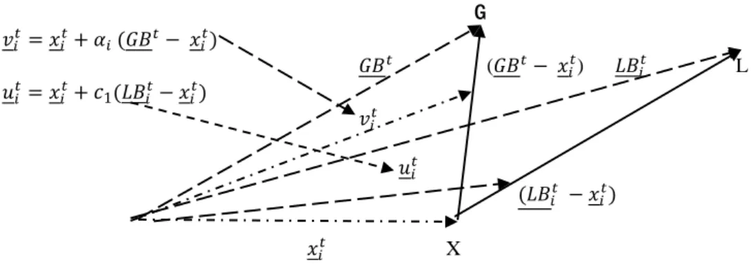
In making decision about its next position , the ith seeker (for i=1,2,.. populationSize) considers adjusting its current position to (i.e moving to a neighbouring shop) and then moving along the direction ( ) to select the point,
( ) ( )
where is a diagonal matrix for some diagonal entries. This is obtained by noting that can be written as for some diagonal matrix . The addition of (which can be random or otherwise) provides way of enhancing diversification or explorative process. Since I+D’ is still arbitrary due to arbitrariness of D’ we could equal write the above as
( )
for a diagonal matrix D. This position is now compared with the position
obtained by moving in the direction from its current position . The better of the position in terms of the fitness value is then selected:
{ ( ) ( )
However if the position selected is too close to the current global optimum, the seeker, (driven by the desire to be relevant, compete, or improve on the current point ) may launch out to explore other points in the space ( generating its position randomly) other than those in the directions ,( ).
By this act the explorative process of the algorithm is enhanced.
G
( ) L
X
Figure 1. A show of directions of movement of a particle for the case with =0
Based on the model the following algorithm results. The Algorithm
With the following parameters as defined,
: positive constants probably in the range [2,4]. In this experiment, , = 3.5 are used.
dim : the dimension of the problem.
rand() : a random number generator that returns a random number in the range [0,1] : a vector denoting the position of particle i at time k (i.e at kth iteration)
: a vector denoting the global best position (among all the particles) ever attained up to time k .
: a vector denoting the best position up to time k ever attained by particle i
: the geometric distance of position from
minx =( minx1, minx1, ….., minxdim , maxx =( maxx1, maxx1, ….., maxxdim )
where minxj, maxxj (for j=1,2..,dim) are respectively the lower and upper bound for value of component j of
fitValue( z ): the fitness value of position z.
: the bound on the distance of the particle from the current global position below which particles generate
their position randomly The value =10-10 is used in this experiment.
The algorithm is thereby stated as follows, Initialization step:
a. INITIALIZE randomly the positions of all the particles in the population:
, for i=1,2…,noOfParticles
b. COMPUTE the fitness value, fi =fitValue( ), of each particle’s position (for i=01,2,…noOfParticles).
Iterative step:
for k=1,2,……….noOfIterations do the following looping for ( i=1 ,….., noOfParticles ) do the following
{ (i)UPDATE xik to obtain xik+1 :
a.
b. ( )
( with any component of or out of interval bound generated randomly as in step (a) of initialization step)
c. If (fitValue(v) >fitValue(u)) then set else set ;
d. if ( distance( , ) < ) then (ii) UPDATE global best position GB to obtain and the fitness value of :
if ( fitValue( ) < fitValue( )) then set = else =
1.2. Output
The current global best position, , and its fitness value, fitValue( ).
2. RESULTS of TEST EXPERIMENT and DISCUSION
The proposed algorithm was implemented in Java using Netbeans 5.0 and tested on many existing benchmark functions devised for optimization search algorithms. The benchmark functions may be grouped according to whether they are unimodal (U) having one global optimum point , multimodal (M) have many local optimum points and separable(S) being expressible as a sum of functions each of which is a function of one variable. Having this in mind the following benchmark functions were considered for presentation with results obtained placed on the Tables. The minimization problem is turned into optimization problem by negating the objective function (i.e min{F(x)} is turned into max{-F(x)} ).
F0: Rosenbrock’s(UN): ∑ [ ]. Global Min: 0 at =1 in [-3,3] d.
F1: De Jong’s ∑ . Global Min:0 at (0,0,…..,0) in [-10,10] d.
F2: Schwefel (UN) ∑ (∑ ) . Global Min:0 at (0,0,..,0) in [-10,10] d.
F3: Eggerate : . Global Min:0 at (0,0,..,0) in [-2π, 2π]2
.
F4: Ackley’s (MN) ( √ ∑ ) ∑
Global Min:0 at point (0,0,…..,0) in [-10,10] d.
F5: Griewank (MN): ∑
∏ √ . Global Min :0 at (0,0,…,0) in [-10,10] d.
F6:
∑
∏ √
F7 Rastrigin (MS): ∑ .Global Min:0 at (1,1,..,1)
in [-10,10] d.
F8 Schwefel(MS): – ∑ √ . Global Min:0 at
=420.9867 in [-500,500] d.
F9 Styblinski-Tang(): ∑ .Optimum. value:39.165999*d at =-2.903534
F10 Dixon-Price (MS): ∑ .Global Min:0, in [-10,10]d
F11 Zakharov(MS): ∑ ∑ ∑ . Global Min:0 at =0 in [-5,10] d.
F12 Trial 6 (MS): ∑ ∑ . Global Min:-50 for d=6,-200 for d=10, in [-d2,d2]d.
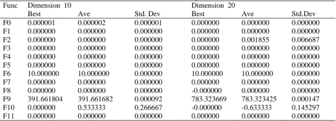
Tables 1, 2 present the results obtained from the method on the these functions but with the dimension 10,20,30,40 and population size 20. The average best ( ave. Best), average (Ave) and the standard deviation (Std. Dev) of fitness values were computed over 20 runs of the algorithm with each run comprising of 50,000 iterations over the particle population.The parameter values D=[ ] (with = 2.4 here for all i) , , = 3.5 , = 10-10 were used in the test.
The algorithm attains the global optimum for all the functions except on F10 for dimension above 20 to which the algorithm converges to 0.666667 instead of the optimum 0. Although for dimension 40 the algorithm fails to reach the optimum for function F2 for population size 20 and 50 000 iterations it does reach it when the population and the number of iterations were increased to 70 and 500 000 respectively (see Table 3).
Table 1. Result comparing the algorithm with PSO for Dimension = 10 population = 20 with 50 000 iterations per run
Func Dimension 10 Dimension 20
Best Ave Std. Dev Best Ave Std.Dev
F0 0.000001 0.000002 0.000001 0.000000 0.000000 0.000000
F1 0.000000 0.000000 0.000000 0.000000 0.000000 0.000000
F2 0.000000 0.000000 0.000000 0.000000 0.001855 0.006687
F3 0.000000 0.000000 0.000000 0.000000 0.000000 0.000000
F4 0.000000 0.000000 0.000000 0.000000 0.000000 0.000000
F5 0.000000 0.000000 0.000000 0.000000 0.000000 0.000000
F6 10.000000 10.000000 0.000000 10.000000 10.000000 0.000000
F7 0.000000 0.000000 0.000000 0.000000 0.000000 0.000000
F8 0.000000 0.000000 0.000000 -0.000000 0.000000 0.000000
F9 391.661804 391.661682 0.000092 783.323669 783.323425 0.000147
F10 0.000000 0.533333 0.266667 -0.000000 -0.633333 0.145297
F11 0.000000 0.000000 0.000000 0.000000 0.000000 0.000000
Table 2. Result for Dimension=30, 40 population = 20 with 50 000 iterations per run
Fuc Dimension:30 Dimension: 40
Best Ave Std.Dev Best Ave Std.Dev
F0 0.000237 6.837006 8.143482 0.037839 17.211248 9.353196
F1 0.000000 0.000000 0.000000 -0.000000 -0.000000 0.000000
F2 0.000000 2229.653809 1231.072388 1628.177368 4119.499023 1432.933960
F3 0.000000 0.000000 0.000000 0.000000 0.000000 0.000000
F4 0.000000 0.000000 0.000000 0.000000 0.000000 0.000000
F5 0.000000 0.000000 0.000000 0.000000 0.000000 0.000000
F6 10.000000 10.000000 0.000000 10.000000 10.000000 0.000000
F7 0.000000 0.000000 0.000000 0.000000 0.000000 0.000000
F8 0.003906 0.003906 0.000000 0.009766 0.009766 0.000000
F9 1174.98571 1174.985596 0.000281 1566.648315 1566.647705 0.000391
F10 0.666667 0.666667 0.000000 0.666667 3.235879 9.577686
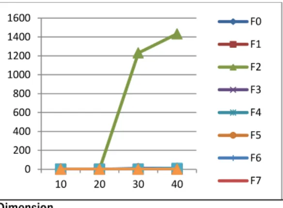
Figure 2 presents a graph showing the performance of the algorithm with respect to the increase in the dimension of the functions with the population size and number of iterations fixed at 20 and 50 000 respectively. It is a plot of the standard deviation of the fitness values against the functions’ dimension. Except on F2, the graph shows that the performance of the algorithm on these other functions is not much affected with this increase in the function’s dimension. But For F2, the number of iterations had to be increased to improve performance as the dimension increases beyond 20.
Dimension
Figure 2. A graph of standard deviation of fitness values of the functions against the dimension of the functions population:20, number of iterations:50000
The graph in Figure 3 (that contains a plot of standard deviation against the number of iterations) shows the effect of increase in the number of iterations on the algorithm with dimension fixed at 10. The graph appears to lend credence to this view that an improvement in the result may sometimes be attained with more iterations.
No of iterations
Figure 3. A graph of standard deviation of fitness values of the functions against the number of iterations for dimension 10, population 20
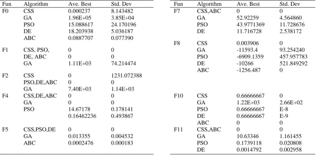
The graph also shows that about 5000 iterations are needed to get reasonable result for these functions.Table 4 below presents the result from the popular algorithms genetic algorithm (GA),Differential evolution(DE), artificial bee colony (ABC) as recorded in [19,20] for population size 50 and 500 000 iterations on some benchmark functions. Also presented on the table is the result of the cheapeastShopSeekers (CSS) (but for population 20, and 50 000 iterations) for comparison. Those algorithms with the best results for those functions are written in bold.
0 200 400 600 800 1000 1200 1400 1600
10 20 30 40
F0 F1 F2 F3 F4 F5 F6 F7
0 50 100 150 200 250 300
500 1000 2000 5000
100
00
200
00
300
00
400
00
500
00
F0 F1 F2 F3 F4 F5 F6 F7
Table 4. comparing results of the algorithm with those of other popular algorithms CSS (population:20, iterations:50 000), GA,PSO,DE,ABC (population:50 iterations: 500 000) Dimension:30
Fun Algorithm Ave. Best Std. Dev Fun Algorithm Ave. Best Std. Dev
F0 CSS
GA PSO DE ABC 0.000237 1.96E+05 15.088617 18.203938 0.0887707 8.143482 3.85E+04 24.170196 5.036187 0.077390
F7 CSS,ABC
GA PSO DE 0 52.92259 43.9771369 11.716728 0 4.564860 11.728676 2.538172
F8 CSS
GA PSO DE ABC 0.003906 -11593.4 -6909.1359 -10266 -1256.487 0 93.254240 457.957783 521.849292 0
F1 CSS, PSO, DE, ABC GA 0 0 1.11E+03 0 0 74.214474
F2 CSS
PSO,DE,ABC GA 0 0 7.40E+03 1231.072388 0 1.14E+03 F4 CSS,DE,ABC
GA PSO 0 0 14.67178 0.16462236 0 0 0.178141 0.493867
F10 CSS
GA PSO DE ABC 0.66666667 1.22E+03 0.66666667 0.66666667 0 0 2.66E+02 E-8 E-9 0 F5 CSS,PSO,DE
GA ABC 0 0.013355 0.0002476 0 0.004532 0.000183
F11 CSS,ABC GA PSO DE 0 10.63346 0.1739118 0.0014792 0 1.161455 0.020808 0.002958
The algorithm is able to match these algorithms (in terms of results) even with population size 20 and 50 000 iterations (being among the best for these functions even for that population size and the number of iterations) except for function F10 where the algorithm fails to reach the optimum (rather hanging at 0.666667) for dimension greater than 20.
3. CONCLUSION
In this paper a population based meta-heuristic algorithm for optimization problems is presented. The algorithm, called cheapest shop seeker, is modeled to mimic a group of shoppers cooperatively seeking for the cheapest shop for shopping.The algorithm is tested over some benchmark functions with dimension 10,20.30, 40 and some of the results are presented on the table above. The graphs depicting its tolerance to dimension increase (at least up to 40) and its sensitivity to the number of iterations required to attain optimum are also presented. A comparison of the results the algorithm produced on these functions and those recorded in [19,20] for genetic algorithm(GA), particle swarm optimization (PSO), Differential evolution (DE) and artificial bee colony(ABC) was also made and presented.The algorithm appears to have a better success rate of reaching the global optimum point and with fewer number of iterations required to attain it.The simplicity of the algorithm compared with some of these algorithms is another feature of the algorithm.
REFERENCES
[1] Wolpert D. H, Macready W. G(1997), “No free lunch theorem for optimization”; IEEE Trans. Evol. Comput. 1997:1:67-82.
[2] Bianchi,Leonora, M Dorigo and others (2009) “A survey on metaheuristic for stochastic combinational optimization” Natural computing: an international Journal 8 (2):239-289
[3] R.S.Parpinelli And H.S. Lopes (2011), New inspirations in swarm intelligence: A survey, International Journal of Bio-inspired computation Vol 3. No. 1 2011 pp1-15
[4] Kennedy J. and Eberhart J. (1995) Particle swarm optimization. In Proc. IEEE International Conference Neural Networks , Piscataway, NJ, vol 4, 1995, pp 1942-1948.
[5] Reynolds C.W(1987).Flocks, herbs and schools: A distributed behavioral model, Proceedings on computer Graphics-ACM SIGGRAPH ’87, vol 21 No 4 pp25-34
[6] Rashedi E. and others (2009) GSA: a gravitational search algorithm . Information sciences 179(13):( 2232-
2248.2009)
[7] Albert Y.S. Lam and Victor O.K.Li(2009) Chemical-Reaction-Inspired Metaheuristic for optimization, Technical Report TR-2009-003, Dept of Electrical & Electronic Engineering, The University of Hong Kong.
[8] Y.Tan and Y. Zhu (2010) “Fireworks algorithm for optimization”, Advances in Swarm Intelligence. LNCS, vol. 6145, pp. 355-364
[9] S.Zheng, J.A., and Y.Tan,(2013) “Enhanced fireworks algorithm”, in Proc. Of the 20134 IEEE Congress on Evolutionary Computation (CEC 2013), pp.2069-2077
[10]Cheng M & Prayogo D. (2014) Symbiotic Organisms search: A new metaheuristic optimization algorithm, Computers and Structures 139 pp 98-112
[11]Iztok Fister Jr and others (2013) A Brief Review of Nature-inspired Algorithms for optimization, ELEKTROTEHNISKI VESTNIK 80 (3) (2013) English edition.
[12]Veenu Mangat(2010) Swarm Intelligence Based Technique for Rule mining in Medical Domain,International Journal of Computer application (0975-8887) vol 4 N0 1, July 2010
[13]Tiago Sousa and others (2004) Particle Swarm based Data Mining Algorithms for classification tasks, Parallel Computing 30 (2004) 767-783
[14]Sadollah A., Bahreininejad A., Eskandar H., Hamdi M. (2013) Mine blast algorithm: A new population based
algorithm for solving constrained engineering optimization problems , Applied soft computing 13 pp 2592-2612
[15]Yang X.S., Deb S (2010) Engineering optimization by Cuckoo search, Int. J. Mathematical Modelling and Numerical optimization, 1(4): 330-343.
[16]Cupic M, Golub M. , Jakobovic D(2009) Exam Timetabling using Genetic algorithm, Proceeding of ITI 2009 31 Int. Conf, on Information Technology interfaces June 22-25, 2009 Cavtat, Croatia. [17]Hybrid Genetic Algorithm and TABU Search Algorithm to solve class Time Table Scheduling
Problem, International of Research studies in Computer Science and Engineering (IJRSCSE) volume 1, issue 4, August 2014 pp19-26
[18]Edmund K. Burke and others(2008) A hybrid heuristic ordering and variable neighbourhood search for the nurse rostering problem, European Journal of Operation research 188(2008) 330-341
[19]Dervis Karaboga, Bahriye Akay(2009), Comparative study of Artificial Bee Colony Algorithm, Applied Mathematics . and computation 214 (2009) 108-132],
[20]Dervis Karaboga & Bahriye Basturk(2007) A powerful and efficient algorithm for numerical function optimatization: artificial bee colony (ABC) algorithm, J. Glob optim 39:459-471 Dol 10.1007/s10898-007-9149-X.