Sharif University of Technology
Scientia IranicaTransactions E: Industrial Engineering www.scientiairanica.com
A two-stage stochastic programming model for
value-based supply chain network design
H. Badri
a, S.M.T. Fatemi Ghomi
a;and T.H. Hejazi
ba. Department of Industrial Engineering, Amirkabir University of Technology, 424 Hafez Avenue, Tehran, P.O. Box 1591634311, Iran.
b. Young Researchers and Elite Club, Qazvin Branch, Islamic Azad University, Qazvin, Iran. Received 6 May 2014; received in revised form 18 November 2014; accepted 10 March 2014
KEYWORDS Supply chain network design;
Value-based management; Two-stage stochastic programming; Correlated parameters.
Abstract.Nowadays, Value-based Supply Chain Management (VbSCM) is considered a resource of competitive advantages, and companies with long term strategic plans nd the VbSCM an eective factor in sustainability. In this context, supply chain network design has a signicant impact on all value drivers (i.e. sales, supply chain costs, xed assets and working capital). This paper proposes a stochastic mixed integer linear programming model for a value-based supply chain network design in which decisions on physical ow (raw materials and nished products) and nancial ow are integrated. The proposed model is designed for a four-echelon, multi-commodity, multi-period supply chain, and it maximizes the value of the company, based on the economic value-added concept, by making some strategic and tactical decisions aecting the value drivers. Furthermore, a scenario-based two-stage stochastic programming model is developed with a scenario generation method based on Nataf transformation. Also, a computational analysis is undertaken to illustrate the performance of the proposed approach.
© 2016 Sharif University of Technology. All rights reserved.
1. Introduction
In the past decade, the concept of Value-based Man-agement (VbM), whose core objective is to increase the value of a rm, has been applied to supply chain management and is known as Value-based Supply Chain Management (VbSCM) [1-4]. In this approach, the value of a company is calculated by its ability to create future cash ow, which, in turn, is driven by protability, capital eciency and cost of capital [5,6]. Furthermore, protability, capital eciency and cost of capital are aected by management decisions of operations, investment and nancing [1,7].
In Supply Chain Network Design (SCND), con-guration of a supply chain requires dierent strate-gic and tactical decisions, such as facility location,
*. Corresponding author. Tel.: +98 21 64545381;
E-mail address: [email protected] (S.M.T. Fatemi Ghomi)
technology selection and production, and distribution planning. These decisions have a long-lasting eect on the survivability of a rm. Furthermore, most of these strategic and tactical decisions are highly correlated with nancial ow in the supply chain.
In classical supply chain network design, it is usually assumed that the value of a company is aected only by its sales or costs [8-10]. Based on this assump-tion, other important value drivers, such as working capital and xed assets, are ignored in the design and planning process. But, based on the VbSCM approach, all value drivers are taken into consideration. From this point of view, supply chain management inuences company value via four nancial drivers, including sales, cost, working capital and xed assets. All decisions made by the management system in nancing, investing and operating aect the value drivers.
Table 1. Structure of the stochastic models in supply chain network design.
Paper SCM
level
Location level
Production stage Time period Final products Objective function Single Multiple Single Multiple Single Multiple
Aghezzaf [8] 2 1 X X X TCa
Ambrosino and Scutell
[9]
3 3 X X X TC
Chan et al.
[18] 1 1 X X X TC
Melkote and
Daskin [19] 2 1 X X X TC
Guillen
et al. [16] 2 2 X X X MO
Hwang [20] 2 1 X X X TC
Lieckens and
Vandaele [21] 2 1 X X X TNP
b
Lowe
et al. [22] 1 1 X X X TC
Miranda and
Garrido [23] 2 1 X X X TC
Miranda and
Garrido [24] 2 1 X X X TC
Pishvaee and
Torabi [10] 3 3 X X X TC
Sabri and
Beamon [17] 3 2 X X X MO
c
Shen and
Qi [25] 1 1 X X X TC
Snyder
et al. [26] 1 1 X X X TC
Ommeren
et al. [27] 2 1 X X X TC
This paper 3 2 X X X EVA
aTC: Total Cost;bTNP: Total Net Prot;cMO: Multiple Objective.
been proposed for VbSCM in which some elements, such as revenue growth, operating costs or operat-ing capital, are considered value drivers [11-14]. In comparison to these conceptual models for VbSCM, a limited number of endeavours have been undertaken concentrating on quantitative models [1,3,15].
In the literature of SCND, there are several stochastic models developed to help managers in con-guration of their supply chain. Most of the proposed stochastic models for SCND are categorized as static models in which decisions are made for a single period. In contrast, there are few multiple period models developed for SCND [8-10]. Production in all reviewed papers is supposed to be done in a single stage. Most of the reviewed papers have considered a single product, but a few have considered multiple products. When it comes to the objective function, total cost is
the most prevalent objective function in the reviewed papers [16,17]. Also, some papers considered multiple objectives in their proposed model. Table 1 shows the structure of the reviewed stochastic models in the eld of SCND.
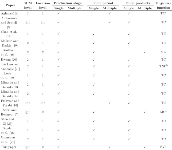
Production planning, inventory management and capacity planning are the most prevalent decisions in the stochastic models of SCND. Also, routing has been considered in a few papers [9,18,20]. From four value drivers proposed by Rappaport [7], supply chain costs have been considered in all reviewed models; but none of the reviewed papers have considered three remaining value drivers, i.e. sales growth, working capital and xed assets. Table 2 illustrates decisions in the reviewed models in the eld of SCND.
This paper proposes a two-stage programming model for value-based supply chain network design.
Table 2. Decisions in the stochastic models in supply chain network design.
Paper Decisions
Procurement Production planning
Inventory management
Capacity planning
Finance, asset management,
and pricing
Routing
Aghezzaf [8] X X
Ambrosino and
Scutell [9] X X
Chan et al. [18] X
Melkote and
Daskin [19] X
Guillen et al. [16] X X X
Hwang [20] X
Lieckens and
Vandaele [21] X X
Lowe
et al. [22] X X
Miranda and
Garrido [23] X
Miranda and
Garrido [24] X
Pishvaee and
Torabi [10] X
Sabri and
Beamon [17] X
Shen and
Qi [25] X
Snyder
et al. [26] X
Ommeren
et al. [27] X X
This paper X X X X X
The proposed model considers both strategic and tactical decisions in the supply chain. The objective of the proposed model is to maximize the value of the company during the planning horizon. For this purpose, four value drivers are considered: supply chain costs, sales growth, working capital, and xed assets. The proposed model covers decisions in operations, nancing and debt management.
Furthermore, in the proposed model, a four-echelon supply chain is considered, including suppliers, production facilities, distribution centers and customer zones. All products are manufactured in a single stage. Also, two kinds of warehouse are considered, a warehouse inside the production facilities for storing raw materials, and a warehouse in distribution centers for the nished products. In this network, nished products should be shipped to the customer zones from the distribution centers, and they cannot be transported directly from the production facilities to the customer zones. Figure 1 illustrates the structure
Figure 1. Structure of the considered supply chain.
of the supply chain considered in the proposed model. It is easily seen in this network that the company owns all production facilities and distribution centers.
The most important assumptions in the proposed model are as follows:
- Customer demand and associated prices are stochas-tic parameters with correlated behavior;
- The total number of distributed products in a market
cannot violate the predicted demand for that time period;
- Short term debt is considered the main source of
nancing;
- An opened facility cannot be closed during the
planning period;
- The capacity of manufacturing facilities is
deter-mined by the amount of installed manufacturing equipment;
- Transfers are not permitted between warehouses;
- All manufactured products are distributed through
distribution centers;
- Depreciation is only considered for the
manufactur-ing equipment;
- Safety stock is required for both raw materials and
nished products;
- Raw materials are stored in manufacturing facilities, and nished products are stored in distribution centers.
Some of the most important decisions in the proposed model are as follows:
- Location and establishment time of facilities
(pro-duction plant, warehouse);
- Amount of manufacturing equipment to be installed
in each facility in each period;
- Total amount of each type of raw material to be
supplied by each potential supplier;
- Total number of each product to be produced in each
manufacturing facility;
- Total number of each nished product transported
from each manufacturing facility to each distribution center;
- Financing decisions.
The remaining part of the paper is organized as follows: The next section includes the proposed mathematical programming model. Section 3 presents the two-stage stochastic programming approach. Com-putational analysis is presented in Section 4, and nally, conclusions are drawn is Section 5.
2. Mathematical programming model
This section proposes a Mixed Integer Linear Program-ming (MILP) model for the VbSCND in a multiple ech-elon, multiple commodity, and multiple period supply chain.
Notations Sets
T (tT , t = t0; :::; T ) ( T ) Set of time periods;
S(sS) Set of suppliers;
I(iI) Set of production plants and
distribution centers; M(M i) Set of production plants;
W(W i) Set of distribution centers;
C(cC) Set of customers;
P (pP ) Set of products (raw material and
nished products); Pr(Pr P ) Set of raw materials;
Pf(Pf P ) Set of nished products.
Parameters
iwacc Weighted average cost of capital;
itr Tax rate;
id Interest rate for short term debts;
BM A very large number;
Dt
p;c Demand of nished product p in
customer zone c;
COPt
p Cost price;
bvt Net book value at the end of lifetime
period t;
sv Salvage value of technical equipment;
PV Cp;i Production variable cost in facility i;
SVMp;i Storage variable cost for raw materials
in production facilities;
SVWp;i Storage variable cost for nished
products in distribution centers;
CAP Capacity of each unit of manufacturing
equipment; Cot
i Fixed cost for opening facility i in
period t;
CUi Fixed cost of operating facility i;
Bp;r Quantity of raw material, r, necessary
to produce a unit of product p (bill of materials);
ICAPi Capacity for storage at production
facility/distribution center;
ISp Space occupied by unit raw material or
nished product;
MSTD Maximum available short term debts
in each period; PRt
p;c Price of a unit of nished product p;
PSt
p Price of a unit of raw material p;
TCp;s;i Transportation variable cost for raw
material p to be transported from supplier s to production facility i;
TCp;i;i0 Transportation variable cost for
nished product p to be transported from production facility i to distribution center i0;
TCp;i;c Transportation variable cost for
nished product p to be transported from distribution center i to customer zone c;
Ai;j Number of deliveries from node i to
node j in one period;
ICASH Position of cash at period t0;
Ihp Position of inventory at period t0;
p Coecient for safety stock of raw
material p;
p Coecient for safety stock of nished
product p;
SHt Stockholder share.
Decision variables
EVA Economic Value Added;
NOPAT Net Operating Prot After Tax;
NOA Net Operating Assets;
TCMt Total Contribution Margin in period t;
DEPt Depreciation and capital loss of
disinvestments in period t;
FA Fixed Assets;
MEQt;i Stock of manufacturing equipment
at location i at the end of period t acquired in period ;
hmt
Pr;i Inventory of raw material Pr in
manufacturing facility i at the end of period t;
hwt
Pf;j Inventory of product Pf in distribution
center j at the end of period t;
ARt Account Receivable;
APt Account Payable;
CASHt Cash in period t;
CFOt Cash Flow from Operations;
CFIt Cash Flow from open Items;
CFSt Cash Flow from Short term nancial
investment;
CFAt Cash Flow from xed Assets;
CFDt Cash Flow from Debt management;
CAt Current net Assets at the end of
period t; ft
Pr;s;i Flow of raw material from supplier
s to manufacturing facility i at the beginning of period t;
ft
Pf;i;j Flow of raw material from
manufacturing facility i to distribution center j at the beginning of period t; ft
Pf;j;c Flow of raw material from distribution
center j to customer c at the beginning of period t;
xt
i Binary variable, 1, if a facility
(production facility/ distribution center) is open in location i in period t, otherwise, 0.
Objective function
Shareholder value is created when earnings exceed total costs of invested capital [7]. Among dierent metrics, Economic Value Added (EVA) is the most prevalent metric of value-based performance [1,3,15]. Therefore, the objective function in the proposed model is to max-imize the EVA over the time periods computed by Net Operating Prot After Tax (NOPAT) in period t minus total costs of invested capital in Net Operating Assets (NOA) at the end of the previous period, adjusted by the weighted average cost of capital (iwacc) [28]. Eq. (1)
shows the objective function in which economic value added is maximized:
Maximize EVA =XT
t=t0
(TCMt DEPt):(1 itr)
T
X
t=t0
fat 1+X
i2M =t 1X
=t0
MEQt;i :(bvt 1 +sv)
+ CAt 1
!
:iwacc: (1)
Constraints
Eqs. (2)-(6) dene elements of the objective function. In Eq. (2), depreciation of the manufacturing equip-ment is calculated and invested capital in xed assets is calculated in Eq. (3). Eq. (4) is related to current assets, including inventories, accounts receivable and cash, minus accounts payable. In Eq. (5), the total con-tribution margin is calculated by subtracting total costs from total sales. Cost elements in this equation are xed cost of operating facilities, supply variable cost, production variable cost, storage variable cost for raw materials, storage variable cost for nished products, and transportation variable cost between supplier and production facilities, between production facilities and distribution centers and between distribution centers and customer zones.
DEPt=X
i2M t 1
X
=t0
FAt= X 8i2M[W
Cot
i:xti 8tT ; (3)
CAt= X
p2Pf
X
i2W
COPt
p:htp;i+ ARt APt+ CASHt
8tT ; (4)
TCMt= X
p2Pf X i2W X c2C PRt p;c:fp;i;ct
X
i2M[W
CUi:xti
X p2Pr X s2S X i2M PSt p:fp;s;it
X
p2Pf
X
i2M
X
i02W
PVCp;i:fp;i;it 0
X
p2Pf
X
i2W
SVMp;i: hwp;jt +
X
i02M
1 2Ai0;i:f
t p;i0;i
!
X
p2Pr
X
i2M
SVWp;i: hmtp;i+
X
s2S
1 2As;i:f
t p;s;i ! X p2Pr X s2S X i2M
TCp;s;i:fp;s;it
X
p2Pf
X
i2M
X
i02W
TCp;i;i0:fp;i;it 0
X p2Pf X i2W X c2C
TCp;i;c:fp;i;ct
+ X
p2Pr
X
i2M
PSt
p:(hmtp;i hmt 1p;i )
+ X
p2Pf
X
i2W
PRt
p;c:(hwp;it hwp;it 1)
8tT : (5)
Eqs. (6) and (7) dene the position of accounts receiv-able and accounts payreceiv-able in each period, respectively:
X p2Pf X i2W X c2C PRt
p;c:fp;i;ct ARt= 0
8tT ; (6)
X p2Pf X i2W X c2C COPt
p:fp;i;ct APt= 0
8tT : (7)
Eq. (8) is to ensure the equilibrium of nancial ow in
the supply chain in each period:
CASHt=CASHt 1 CFOt SHt+ CFIt
+ CFSt+ CFAt+ CFDt
8tft0+ 1; ; T g: (8)
In Eq. (9), operating cash ow in each period is calculated:
CFOt= X
i2M[W
CUi:xti+
X p2Pr X s2S X i2M PSt p:fp;s;it
+ X
p2Pf
X
i2M
X
i02W
PVCp;i:fp;i;it 0
+ X
p2Pf
X
i2W
SVMp;i: hwp;it +
X
i02M
1 2Ai0;i:f
t p;i0;i
!
+ X
p2Pr
X
i2M
SVWp;i: hmtp;i+
X
s2S
1 2As;i:f
t p;s;i ! + X p2Pr X s2S X i2M
TCp;s;i:fp;s;it
+ X
p2Pf
X
i2M
X
i02W
TCp;i;i0:fp;i;it 0
+ X
p2Pf
X
i02W
X
c2C
TCp;i0;c:fp;it 0;c
+ t 1X
=t0
X
i2M
X
i02M
RLCi;i0:RLt;i;i0 = 0 8tT : (9)
Eq. (10) denes cash ow from open items, which is the amount of accounts receivable minus the amount of accounts payable in the previous period:
CFIt= ARt 1 APt 1
8tft0+ 1; ; T g: (10)
Cash ow from nancing, based on short term debt, is calculated in Eq. (11). In Eq. (12) the amount of short term debt borrowed in each period is restricted to the maximum debts available:
CFSt= STDt 1:(1 + id) STDt
8tft0+ 1; ; T g; (11)
STDt MSTD 8tT : (12)
CFAt= X i2M
MEQt;ti :(bv0+ sv)
X
i2M[W
Cot
i:(xti xt 1i )
8tft0+ 1; ; T g: (13)
Constraints (14)-(16) are related to the equilibrium of ows of raw materials and nished products in production facilities and distribution centers, respec-tively. The quantity of nished product stored at the beginning of the current period, plus the total quantity of the same product delivered to the distribution center during the current period, should be equal to the quantity of that product transported to customer zones plus the quantity stored at the beginning of the next period. Also, the quantity of raw material stored at the beginning of the current period, plus the total quantity of the same raw material delivered to a production facility during the current period, should be equal to the quantity of that raw material used to manufacture products during the current period plus the quantity stored at the beginning of the next period.
hwt 1 p;i0 +
X i2M ft p;i;i0 X c2C ft
p;i0;c hwtp;i0 = 0
8i02 W; 8p 2 P
f; 8tft0+ 1; ; T g; (14)
ht 1 p;i + X s2S ft p;s;i X p2Pf X
i02W
BPf;p:fp;i;it 0 htp;i= 0
8i 2 M; 8p 2 Pr; 8tft0+ 1; ; T g; (15)
ht p;i
X
s2S
ft
p;s;i= 0 8i 2 M; 8p 2 Pr; 8t = t0:
(16) Constraints (17) and (18) are related to the storage capacity of raw material in the production facilities, as well as nished product in the distribution centers. Maximum production capacity, based on the number of installed manufacturing equipment, is calculated by Eq. (19). Also, the maximum amount of installable manufacturing equipment in each production facility is determined in Constraint (20):
X
p2Pf
ISp: hwp;it 0+
X
i2M
1 Ai;i0:f
t p;i;i0
!
ICAPi0:xti0
8i02 W; 8tT ; (17)
X
p2Pr
ISp: hmtp;i+
X
s2S
1 As;i:f
t p;s;i
!
ICAPi:xti
8i 2 M; 8tT ; (18)
X
p2Pf
X
i02W
W Lp;i:fp;i;it 0
t 1
X
=t0
CAP:MEQt;i
8i 2 M; 8tft0+ 1; ; T g; (19)
t
X
=t0
MEQt;i MEQMAX
i 8i 2 M; 8tT : (20)
The safety stock of raw material and nished products are calculated by Constraints (21) and (22), respec-tively:
hmt 1 p;i p:
X
p2Pf
X
i02W
Bp;Pr:fp;i;it 0
8i 2 M; 8p 2 Pr; 8tft0+ 1; ; T g; (21)
hwt 1 p;i p:
X
c2C
ft p;i;c
8i 2 W; 8p 2 Pf; 8tft0+ 1; ; T g: (22)
Constraints (23)-(25) guarantee that only opened facil-ities receive or send products:
X
p2Pf
X
i02W
ft
p;i;i0 BM:xt 1i
8i 2 M; 8tft0+ 1; ; T g; (23)
X
p2Pf
X
i2M
ft
p;i;i0 BM:xt 1i0
8i02 W; 8tft
0+ 1; ; T g; (24)
X
p2Pf
X
c2C
ft
p;i;c BM:xt 1i
8i 2 W; 8tft0+ 1; ; T g: (25)
Based on Constraint (26), the total number of nished products sent to a customer zone in each period is limited to the demand of that market:
X
i02W
ft
p;i0;c Dtp;c 8c 2 C; 8p 2 Pf; 8tT : (26)
Constraint (27) ensures that the established facility will remain open till the end of the planning horizon:
xt 1
i xti 0 8i 2 M [ W; 8tft0+ 1; ; T g:
(27) Constraints (28) and (29) determine the initial value
of cash, as well as the inventory of raw material in the rst period, respectively:
CASHt ICASH = 0 8t = t0; (28)
X
8i2W
hwt
p;i Ihp= 0 8p 2 Pf; 8t = t0: (29)
Constraint (30) requires that xt
i be a binary
vari-able. Constraints (31)-(34) restrict some variables from taking negative values. Constraint (35) attributes customer demand and the selling price of nished products to joint stochastic space:
xt
if0; 1g 8i 2 M [ W; 8tT ; (30)
FAt;DEPt; ARt; APt; CASHt; CFOt; TCMt;
STDt; CAt 0 8tT ; (31)
MEQt;i 0 8i 2 M; 8t; T ; (32)
ft
p;s;i; fp;i;it 0; fp;it 0;c 0
8s 2 S; 8i 2 M; 8i02 W; 8c 2 C; 8tT ; (33)
ht
Pr;i; htPf;i0 0 8i 2 M; 8i02 W; 8tT ; (34)
(Dt
p;c; PRtp;c): (35)
3. Stochastic programming approach
This paper applies an approach based on stochastic programming to consider the underlying uncertainty of the proposed model. Stochastic programming is a well-grounded approach to make proper decisions in a stochastic environment. Stochastic problems have some stochastic parameters with known or empiri-cal distributions. One way to handle this problem is to work with some scenarios obtained from the population of stochastic parameters. The stochastic factors usually appear at some stage or time-period
in the decision process. Accordingly, the optimal
decision should be made at each stage, depending on all scenarios occurred before the current stage. To reach this, a negative correlation coecient has been considered between the price of nished products and the associated demand [29]. The following variables are considered to be scenario dependent:
- Inventory of product Pf in distribution center j at
the end of period t: hwPt;#f;j;
- Flow of raw material from distribution center j to
customer c at the beginning of period t: fPt;#f;j;c;
- Total contribution margin in period t: TCMt;#;
- Cash in period t: CASHt;#;
- Cash ow from operations: CFOt;#
- Current net assets at the end of period t: CAt;#.
where # is the scenario index. Accordingly,
con-straints (4)-(9), (14), (17), (22), (26), (28), and (29) are written for each scenario, as well.
If stochastic factors can be represented by some random variables with known or estimable probabil-ity functions, scenario-based stochastic programming requires samples from their parametric or empirical distribution functions. Several theorems have been presented to analyze multivariate distributions. How-ever, most of them consider an identical distribution function for the multiple correlated variables [30,31]. In some cases, there are several coupled random variables with non-identical probability patterns and generating random samples for them might be of interest. Copula theory and Nataf transformation are two powerful methods introduced for this purpose [32,33].
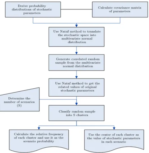
3.1. Scenario generation method
Stochastic programming requires some samples from stochastic parameters that are combined into the sce-narios. Next, each scenario is applied to develop the nal stochastic programming model. In this paper, a method, based on the Nataf transformation, is proposed to generate correlated continuous random variables. The basics of the Nataf method are given below.
Let X = (x1; ; xn) be random variables with
marginal probability distribution functions, f(xi), i =
1; 2; ; n, and correlation matrix, 0. This vector of
random variables can be transformed to a vector of multivariate normal distribution, Y = (y1; ; yn)0
Nn(0; ) by the following equations:
(yi) = F (xi) 8i = 1; 2; ; n; (36)
where (:) denotes cumulative normal probability func-tion and F (:) is the cumulative distribufunc-tion funcfunc-tion of random variables. The elements of are obtained by the following equations:
0 ij=
1
Z
1 1
Z
1
xi i
i
xj j
j
fxixj(xi; xj)dxidxj
=
1
Z
1 1
Z
1
F 1
i ((yi)) i
i
F 1
j ((yj)) j
j
!
'(yi; yj; ij)dyidyj;
8i = 1; 2; ; n; 8j = i; i + 1; ; n: (37)
distribu-Figure 2. Method of scenario generation.
tion can be considered for sample generation. After-wards, the normal variables are again converted to the original variables (X). Figure 2 shows the proposed method of the scenario generation method proposed in this paper.
The main steps of the proposed scenario genera-tion method can be described as follows:
Step 1. Derive marginal distribution functions for original stochastic variables and calculate their covariance matrix. This can be done by gathering historical data from each variable and conducting some non-parametric statis-tical hypothesis tests on goodness of t that can evaluate and select a proper probability distribution function. Chi-square, Anderson-Darling, and Kolmogorov-Smirnov tests are the main methods in attaining this goal [34];
Step 2. Apply marginal distributions and the co-variance matrix in the Nataf transformation algorithm to construct a multivariate normal distribution;
Step 3. Generate samples from the correlated nor-mal distribution; methods such as Cholesky and eigenvector decomposition could be
ap-plied [34]. Such methods are available in most statistical software packages such as Minitab and SAS;
Step 4. Invert the generated normal variables to the original values using Nataf transformation equations.
4. Computational analysis
This section conducts some computational experiments to evaluate the performance of the proposed solution approach. Dierent test problems were designed in three classes, with ve test problems (S1-S5) in the
small class (S), three test problems (M1-M5) in the
medium class (M), and six test problems (L1and L6) in
the large class (L). In the small and medium classes of the test problem, ve instances, and, in the large class of the test problems, six test problems with a dierent number of scenarios (5-30), are generated. Table 3 illustrates the structure of the test problems. For all generated instances, the planning horizon was xed to ve periods, and the number of customers was xed to 10. Demand and price were assumed to be uniformly distributed with known correlation, which could be
Table 3. Structure of the test problems.
Instances Suppliers Manufacturers Warehouses Row material Scenarios Class ID
Small
S1 2 2 1 10 5
S2 2 2 1 10 15
S3 2 2 1 10 20
S4 2 2 1 10 25
S5 2 2 1 10 30
Medium
M1 5 5 5 20 5
M2 5 5 5 20 15
M3 5 5 5 20 20
M4 5 5 5 20 25
M5 5 5 5 20 30
Large
L1 10 10 10 30 5
L2 10 10 10 30 10
L3 10 10 10 30 15
L4 10 10 10 30 20
L5 10 10 10 30 25
L6 10 10 10 30 30
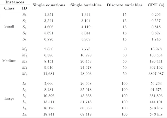
Table 4. Computational results. Instances
Single equations Single variables Discrete variables CPU (s) Class ID
Small
S1 1,351 1,344 15 0.206
S2 3,521 3,194 15 0.557
S3 4,606 4,119 15 0.818
S4 5,691 5,044 15 0.697
S5 6,776 5,969 15 1.746
Medium
M1 2,856 7,778 50 13.978
M2 6,386 16,228 50 103.534
M3 8,151 20,453 50 186.441
M4 9,916 24,678 50 302.192
M5 11,681 28,903 50 3897.987
Large
L1 5,666 26,668 100 56.263
L2 8,281 35,018 100 91.675
L3 10,896 43,368 100 581.896
L4 13,511 51,718 100 444.101
L5 16,126 60,068 100 > 3 hrs
L6 18,741 68,418 100 > 3 hrs
obtained even from the slope of linear relationships (details are provided in the appendix).
These instances were solved using the CPLEX MIP solver. The CPLEX MIP solver was run on a Dual core 2.26 GHz processor with 2 GHz of RAM.
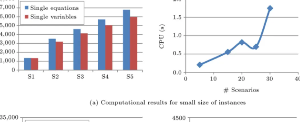
Computational results are shown in Table 4. From the results, we observe that in the small class of instances, the total number of extended equations varies from 1,351 to 6,776, while the total number of variables falls between 1,344 and 5,969. For all instances in this
Figure 3. Computational results for dierent classes of instances.
class, the total number of discrete variables is 15. The CPU time for these instances varies from 0.2 s to 1.7 s, indicating a good performance for this class of problem (see Figure 3(a)).
In the medium class of instances, the total number of equations starts from 2,856 (M1) and reaches 11,681 (M2). Also, the number of single variables for this class of test problem varies from 7,778 to 28,903. Furthermore, the total number of discrete variables for all generated instances in this class is 50. In this class of problems, the increasing trend in the CPU time is signicant, varying from 13.9 s to 3897 s (see Figure 3(b)).
In the large class of instances, the total number of single equations exceeds 18,000. Also, while the minimum number of discrete variables is 26,668 in instance L1, it reaches 68,418 in instance L6. The total number of discrete variables in this class of problem is 100. The CPU time is 56 s for the smallest test problem
in this class (L1), 91 s for L2, 581 s for L3, and 444 for
L4. But, the CPU time in instances L5and L6exceeds
3 h (see Figure 3(c)).
Based on computational results, the adopted ap-proach is ecient for all test problems in the small size class, all test problems in the medium size, and some test problems in the large size. But, for the large size problems with more than 40 nodes (suppliers, manufac-turing facilities, distribution centers, and customers) and more than 25 scenarios, the current approach cannot nd the optimum solution in a reasonable amount of time (3 h).
5. Conclusion
This paper proposes a new stochastic mixed integer linear programming model for the supply chain network problem from a value based approach. To illustrate the position of this approach in the literature and
investigate to what extent the researchers have taken the value based concepts into consideration, an ex-tensive review was conducted on papers in the eld of supply chain network design. Based on the value-based approach, Supply Chain (SC) conguration and planning is undertaken in such a way that the value of SC is maximized. Also, SC costs, sales growth, working capital, and xed assets are supposed to be the main value drivers. Furthermore, it is assumed that customer demand and the selling price of the nished products are stochastic parameters with correlated behavior.
Also a scenario-based two-stage programming ap-proach is developed to consider the underlying uncer-tainty of the proposed model. Within the scenario generation process, Nataf transformation was applied to generate correlated continuous random variables. To evaluate the performance of the developed solution approach, some numerical instances are generated and solved. The results indicate that the developed solution procedure could nd a robust solution in a reasonable amount of time.
References
1. Brandenburg, M., Quantitative Models for Value-Based Supply Chain Management, Springer-Verlag Berlin Heidelberg (2013).
2. Christopher, M. and Ryals, L. \Supply chain strategy: Its impact on shareholder value", International Jour-nal of Logistics Management, 10, pp. 1-10 (1999).
3. Hahn, G.J. and Kuhn, H. \Simultaneous investment, operations, and nancial planning in supply chains: A value-based optimization approach", Intern. Journal of Production Economics, 140(2), pp. 559-69 (2012).
4. Shapiro, J., Modeling the Supply Chain, Second Ed., Thompson (2007).
5. Damodaran, A., The Little Book of Valuation - How to Value a Company, Pick a Stock, and Prot, Wiley (2011).
6. Damodaran, A., Applied Corporate Finance, 3rd Ed., Wiley (2011).
7. Rappaport, A., Creating Shareholder Value: A Guide for Managers and Investors, Second Ed., New York, Free Press (1998).
8. Aghezzaf, E. \Capacity planning and warehouse lo-cation in supply chains with uncertain demands", Journal of the Operational Research Society, 56, pp. 453-62 (2005).
9. Ambrosino, D. and Scutell, M.G. \Distribution net-work design : New problems and related models", European Journal of Operational Research, 165, pp. 610-24 (2005).
10. Pishvaee, M.S. and Torabi, S.A. \A possibilistic programming approach for closed-loop supply chain
network design under uncertainty", Fuzzy Sets and Systems, 161(20), pp. 2668-83 (2010).
11. Christopher, M. and Ryals, L. \Supply chain strategy: Its impact on shareholder value", International Jour-nal of Logistics Management, 10(1), pp. 1-10 (1999).
12. Walters, D. \The implications of shareholder value planning and management for logistics decision mak-ing", International Journal of Physical Distribution and Logistics Management, 29(4), pp. 240-58 (1999).
13. Lambert, D. and Pohlen, T. \Supply chain metrics", International Journal of Logistics Management, 12(1), pp. 1-19 (2001).
14. Otto, A. and Obermaier, R. \How can supply networks increase rm value? A causal framework to structure the answer", Logistics Research, 1, pp. 131-48 (2009).
15. Hahn, G.J. and Kuhn, H. \Value-based performance and risk management in supply chains: A robust optimization approach", International Journal of Pro-duction Economics, 139(1), pp. 135-44 (2012).
16. Guillen, G., Mele, F.D., Bagajewicz, M.J., Espu~na, A. and Puigjaner, L. \Multiobjective supply chain design under uncertainty", Chemical Engineering Science, 60, pp. 1535-53 (2005).
17. Sabri, E.H. and Beamon, B.M. \A multi-objective approach to simultaneous strategic and operational planning in supply chain design", Omega, 28, pp. 581-98 (2000).
18. Chan, Y., Carter, W.B. and Burnes, M.D. \A multiple-depot, multiple-vehicle, location-routing problem with stochastically processed demands", Computers & Op-erations Research, 28, pp. 803-26 (2001).
19. Melkote, S. and Daskin, M.S. \Capacitated facility location/network design problems", European Journal of Operational Research, 129, pp. 481-95 (2001).
20. Hwang, H.-S. \Design of supply-chain logistics system considering service level", Computers & Industrial Engineering, 43, pp. 283-97 (2002).
21. Lieckens, K. and Vandaele, N. \Reverse logistics net-work design with stochastic lead times", Computers & Operations Research, 34, pp. 395-416 (2007).
22. Lowe, T.J., Wendell, R.E. and Hu, G. \Screening loca-tion strategies to reduce exchange rate risk", European Journal of Operational Research, 136, pp. 573-590 (2002).
23. Miranda, P.A. and Garrido, R.A. \Incorporating in-ventory control decisions into a strategic distribution network design model with stochastic demand", Trans-portation Research Part E, 40, pp. 183-207 (2004).
24. Miranda, P.A. and Garrido, R.A. \Valid inequalities for Lagrangian relaxation in an inventory location problem with stochastic capacity", Transportation Re-search Part E, 44, pp. 47-65 (2008).
25. Shen, Z.M. and Qi, L. \Incorporating inventory and routing costs in strategic location models", European
Journal of Operational Research, 179, pp. 372-89 (2007).
26. Snyder, L.V., Daskin, M.S. and Teo, C.-P. \The stochastic location model with risk pooling", European Journal of Operational Research, 179, pp. 1221-38 (2007).
27. Ommeren, J.C.W.V., Bumb, A.F. and Sleptchenko, A.V. \Locating repair shops in a stochastic environ-ment", Computers & Operations Research, 33, pp. 1575-94 (2006).
28. Kaplan, R.S. and Atkinson, A.A., Advanced Manage-ment Accounting, 3rd Ed., Prentice-Hal (1998).
29. Simchi-Levi, D., Kaminsky, P. and Simchi-Levi, E., Designing and Managing the Supply Chain: Concepts, Strategies & Case Studies, McGraw-Hill (2009).
30. Johnson, N.L., Kotz, S. and Balakrishnan, N., Discrete Multivariate Distributions, Wiley New York (1997).
31. Kotz, S., Balakrishnan, N. and Johnson, N.L., Contin-uous Multivariate Distributions, Models And Applica-tions, London: John Wiley & Sons (2004).
32. Liu, P.-L. and Der Kiureghian, A. \Multivariate dis-tribution models with prescribed marginals and covari-ances", Probabilistic Engineering Mechanics, 1(2), pp. 105-12 (1986).
33. Nelsen, R.B., An Introduction to Copulas, New York, Springer (1999).
34. Golub, G.H. and Van Loan, C.F., Matrix Computa-tions, 4th Ed., Baltimore, Johns Hopkins University Press (2012).
Appendix: A procedure for Nataf transformation
Parameters PR = [pr]: Prices; D = [d]: Demands;
(:): Cumulative distribution function of the normal variable.
Inputs
Fpr(pr) = Upr Lpr Lprpr: Cumulative distribution function
of the uniform variable for the price;
Fd(d) = Ud Ld Ldd: Cumulative distribution function of
the uniform variable for the demand;
P0: Correlation matrix between PR and D.
Nataf transformations
Find new normally distributed variables, so that;
1. M = 0; vector of means;
2. P = g(P0); correlation matrix, where g(:) is the
function mentioned before by Eq. (37).
Generate random samples from the multivariate nor-mal distribution; Z N(M; P ).
Convert the generated samples to original vari-ables using Eq. (36).
Biographies
Hossein Badri is a PhD degree candidate in the Department of Industrial Engineering at Amirkabir University of Technology, Tehran, Iran. His research interests are in supply chain network design, multiple criteria decision making, and combinatorial optimiza-tion methods. He is author and co-author of more than 20 technical papers in these elds.
Seyyed Mohammad Taghi Fatemi Ghomi was born in Ghom, Iran, on March 11th, 1952. He received his BS degree in Industrial Engineering from Sharif University of Technology, Tehran, Iran, in 1973, and a PhD degree in the same subject from the University of Bradford, England in 1980. He worked as planning and control expert in construction and cement industries, and the Organization of National Industries of Iran from 1980-1983, where he founded the Department of Industrial Training in 1981. He is currently Professor in the Department of Industrial Engineering at Amirkabir University of Technology, Tehran, Iran, where he was recognized as one of the best researchers of years 2004 and 2006, and best professor at the university in 2014. He was also recognized by the Ministry of Science and Technology as one of the best Professors
of Iran for 2010. He is author and co-author of
more than 350 technical papers and six books in the area of Industrial Engineering, and has supervised 133 MSc and 19 PhD theses. His research and teaching interests are in stochastic activity networks, produc-tion planning, scheduling, queueing theory, statistical quality control, and time series analysis and forecast-ing.
Taha-Hossein Hejazi received his PhD, MS and BS degrees in Industrial Engineering from Amirkabir University of Technology, Shahed University of Tehran, and Sadjad University of Technology, Iran, respec-tively. His primary research areas include quality and reliability engineering, simulation, and multiple criteria analysis. He has also written four books in areas of industrial engineering, such as discrete and continuous system simulation, quality and reliability engineering, and multiple criteria decision making.
![Table 2. Decisions in the stochastic models in supply chain network design. Paper Decisions Procurement Production planning Inventory management Capacityplanning Finance, assetmanagement, and pricing Routing Aghezzaf [8] X X Ambrosino and Scutell [9] X X C](https://thumb-us.123doks.com/thumbv2/123dok_us/8382465.2227087/3.892.83.792.175.930/decisions-stochastic-decisions-procurement-production-inventory-capacityplanning-assetmanagement.webp)