Subcellular processes in morphogen gradient formation studied with 3D-tracking fluorescence microscopy

(1)

Subcellular processes in morphogen

gradient formation studied with

3D-tracking fluorescence microscopy

(2)

(3)

Subcellular processes in morphogen

gradient formation studied with

3D-tracking fluorescence microscopy

Proefschrift

ter verkrijging van

de graad van Doctor aan de Universiteit Leiden, op gezag van Rector Magnificus prof.mr. P.F. van der Heijden,

volgens besluit van het College voor Promoties te verdedigen op dinsdag 8 december 2009

klokke 13.45 uur

door

Laurentius Henricus Franciscus Maria Holtzer

(4)

Promotiecommissie:

Promotor: Prof. dr. T. Schmidt

Referent: Prof. dr. M. González-Gaitán (Université de Genève, Zwitserland) Overige Leden: Prof. dr. P.-R. ten Wolde (AMOLF, Amsterdam)

Prof. dr. N. H. Dekker (Technische Universiteit Delft) Prof. dr. H. P. Spaink

Prof. dr. M. Orrit Prof. dr. T. J. Aartsma Dr. ir. S. J. T. van Noort Prof. dr. J. M. van Ruitenbeek

ISBN 978-90-8593-064-8

Casimir PhD Series, Delft-Leiden 2009-19

(5)

Chapter 1 Introduction

One of the most fundamental questions in life is how an organism grows and develops from a single cell into a fully grown adult. A major step forward in solving this question was the discovery of the molecule that contains all the information needed by an organism: DNA. It was further found that every cell in an organism contains an exact copy of this DNA. This immediately posed another question: how do cells, while having the exact same DNA, know where they are located in the organism and what functions they should perform. How does a cell know whether it is a kidney cell and not a heart or brain cell, and even more, how does it know where it is located within the kidney?

(8)

2 Introduction

1.1 The morphogen gradient

1.1.1 Morphogens

Almost 60 years ago Turing proposed that morphogens are providing the po-sitional information for cells in developing organisms in which they are ex-pressed in all the cells in the tissue [1]. Wolpert in turn proposed that mor-phogens are actually produced by spatially localized special cells. By spread-ing throughout the tissue morphogens form a gradient in the neighborspread-ing cells, the receiving tissue [2]. There the morphogen is detected by receptors on the cell surface. Depending on the morphogen concentration cells will adapt their gene expression pattern. Figure 1.1 shows a schematic drawing of a morphogen gradient.

Most of the models describing morphogen gradients assume, and experi-ments have proven, that the system is in a steady state. The formation of mor-phogen gradients occurs in a much shorter period than the time needed for patterning tissue [3]. In general two models exist that describe a steady mor-phogen gradient in tissue. When degradation takes place at a discrete loca-tion a linear gradient forms [3], while if degradaloca-tion occurs in all the receiving cells, the morphogen gradient will have an exponential shape [4]. Experimen-tally the latter was found to be the case in the wing imaginal disc of the fruit flyDrosophila melanogasterin which the morphogens Decapentaplegic (Dpp) and Wingless (Wg) play an essential role during development of the wing of the fly [5].

1.1.2 Dpp

(9)

1.1 The morphogen gradient 3

[Morphogen]

C1

C2

Gene 1

Gene 2

(10)

4 Introduction

Dpp is a member of the TGF-βsuperfamily and is homologous to the verte-brate Bone Morphogenetic Protein (BMP). Dpp takes part in a major develop-mental signaling pathway. The receptor for Dpp was found to be composed of Thickveins (Tkv) [7] and Punt [8]. After formation of the Dpp-receptor com-plex the intracellular protein Mad (Mothers against dpp) is phosphorylated. Subsequently pMad controls activation of transcription of its target genes opto-motor-blind(omb) andspalt(sal) in a Dpp concentration-dependent manner [9]. Optomotor-blind is a requirement for the development of the wing [10], Spalt plays a role in the formation and positioning of specific veins in the wing [11]. Besides playing a role in the Dpp signaling pathway, the Dpp receptor is also required for Dpp-receptor internalization. This process plays a major role in Dpp spreading and degradation [12–15].

In the wing imaginal disc Dpp is produced at the anterior-posterior com-partment boundary [16] from which it is secreted to the neighboring receiving cells. Dpp forms a steady-state single-exponential gradient which can fully be described by three parameters: the production rate, the diffusion constant and the degradation rate [4].

1.1.3 Morphogen spreading

The spreading of Dpp in the receiving cells has been a subject of study for many years. In most of those studies (confocal) microscopy supplemented with dynamic techniques like fluorescence recovery after photobleaching (FRAP) were combined with sophisticated genetic technologies in order to describe the morphogen gradient and its spreading in terms of a coarse-grained con-centration profile in the tissue. Those experiments suggest that Dpp is spread by three different mechanisms:

1. Diffusion in the extracellular matrix [17]; 2. Receptor-mediated transport [18];

(11)

1.2 Particle tracking in cells and tissue 5

The extracellular diffusion and receptor-mediated transport are governing short-range spreading, while intracellular transport is essential for long-range spreading [20]. Theoretical calculations have estimated that one cycle of intra-cellular transport has a duration between 50 and 150 s [19, 21].

In the current thesis we strive to extend the settled coarse-grained mod-els of intracellular Dpp transport to a more molecular model that involves endosome-mediated Dpp transport. We studied endosome transport by 3D fluorescence microscopy. The experimental approach will be outlined in the next section.

1.2 Particle tracking in cells and tissue

1

For long microscopy has been one of the primary techniques in biological in-vestigation. In particular light microscopy which allows one to directly ob-serve biological processes in vivois used on an every-day’s basis in biology laboratories. One of the characteristics of a systemin vivo- or a live system - is the constant movement of all its components. The mobility of ions, small molecules like ligands, proteins whether membrane-bound [22–29] or located in the cytosol [30–32], and larger assemblies like vesicles [33, 34], the nucleus [35] or viruses [36], is finally determining the way how the system evolves and self-regulates. Hence, in a strive to understand living systems on a microscopic mechanistic basis one wants to characterize the mobility of its components and combine this knowledge to the functional state of the system.

The two main classes of mobility, i.e. unrestrictive diffusion and linear di-rected motion, are rather the exception in the context of the complex envi-ronment of the cell and tissue [37, 38]. Proteins, for example, might for some time diffuse freely through the cytosol. However, due to binding events or restriction in their diffusional space, their mobility may become slowed on longer time and length scales. Likewise a vesicle, which is immobile for an

1_{This section is based on: L. Holtzer and T. Schmidt, Single-Molecule Tracking in Cells}

(12)

6 Introduction

initial phase of observation, could be actively transported at a later phase due to molecular motors which follow a microtubular track [39–42]. Recording and classification of such complex mobility behavior in a statistically signifi-cant manner asks for a signifisignifi-cant and careful effort in technology development and automated analysis tools to render successful.

In what follows we describe the foundations for the technology developed by us and others in order to permit tracking of individual molecules and small molecular assemblies. We will mainly focus on applications in biomembranes, in cells and in tissue, and illustrate by selected examples how biological infor-mation is extracted by a detailed analysis of molecular mobility.

1.2.1 Single-molecule and single-particle localization

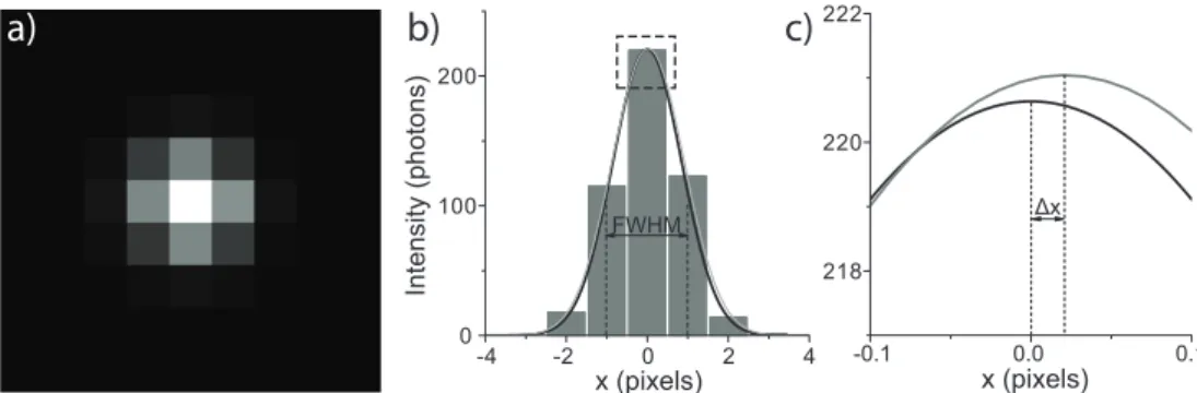
The use of wide-field fluorescence microscopy allows for parallel, hence fast data acquisition. It is therefore the most appropriate technology for track-ing movtrack-ing molecules and objects. In wide-field fluorescence microscopy an isotropic emitter smaller than the diffraction limit will appear as a diffraction limited spot in the image plane [43]. Its image is characterized by a sym-metrical signal distribution around the center with the maximum intensity at the center of the spot. The intensity distribution I(x,y)of such an object on a highly-sensitive CCD camera used in the experiments described, is de-termined by the point spread function (PSF). A good approximation of the PSF is given by a two-dimensional Gaussian with full-width-at-half-maximum (FWHM) equal tow = 1.03λ/NA, withλthe wavelenght of the emitted light and NA the numerical aperture of the microscope objective [22, 44, 45]:

I(x,y) =N4 ln 2

πw2 exp[−4 ln 2((

x−µx)2

w2 +

(y−µy)2

w2 )] (1.1) whereµxandµyare thexandycoordinates of the object, andNthe total

(13)

Identification of individual molecules is complicated by unavoidable back-ground signals in living cells due to out-of-focus objects and autofluorescent particles. Therefore image pre-processing and reliable background removal is necessary. It turned out that background signals are satisfactorily removed by applying a spatial low-pass filter to the image with a cut-off frequency of 5/w, frequencies which are far below the frequencies generated by the objects of interest. Subtraction of the filtered image from the original image reliably yields an image with a zero background. Likewise static objects are faithfully removed using a temporal low-pass filter on the movie stack and subsequently subtracted from the original image. The latter method needs to be applied carefully in order not to remove slowly moving or static objects of interest.

After appropriate background subtraction automatic object identification and position analysis is performed. An easy and fast way to determine the position of the object in the object plane is calculating the center of mass, or centroid, of its image for each axis

µx = My

∑

i=1

Mx

∑

j=1

(xi⋅Ii j)/ My

∑

i=1

Mx

∑

j=1

Ii j (1.2)

whereIi j is the signal at a pixel(i,j)[47, 48]. It is important that the

fluores-cence intensity of the image has no offset, as this will bias the position of the particle towards the center. Advantage of this method is that it does not use any prior knowledge about the shape of the intensity profile and can therefore be applied to objects even in case of imaging errors or to objects which are larger than the diffraction limit [49].

(14)

ac-8 Introduction

a) b) c)

-4 -2 0 2 4 0

100 200

In

te

n

si

ty

(p

h

o

to

n

s)

x (pixels)

FWHM

-0.1 0.0 0.1

218 220 222

x (pixels)

Δx

Figure 1.2:a)Simulated image of a diffraction limited spot approximated by a 2D Gaus-sian intensity profile. Poisson noise was added to account for the stochastic nature of photon emission (w=2 pixels,N=1000).b)Intensity of the image along a horizontal line through the center. In black a 1D Gaussian is shown calculated directly from the input parameters. A fit to the data is shown in gray. c)A closer look at the part of (b) indicated by the square. It can be clearly seen that the Gaussian fit determines the position of the particle with high accuracy (∆x=0.02 pixels).

curacy of<30 nm is achieved at video rate (e.g. a frame rate of 25 Hz) [27, 51].

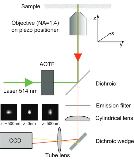
Positional determination as described so far solely allows to extract infor-mation on the lateral positon of an object. In recent years several methods to determine also the axial position have been described [52–60]. A straightfor-ward and cost-effective method to determine thez-position of a single particle is by introducing a slight astigmatism into the detection beampath [50, 61]. A schematic drawing of the experimental setup is shown in fig. 1.3. This method will be extensively described in chapter 2 of this thesis. The axial accuracy which is obtained by using this method is about 2.5 times that of the lateral positional accuracy. Typically<75 nm is achieved in live cell experiments.

(15)

Objective (NA=1.4) on piezo positioner

Dichroic

Emission filter Laser 514 nm

Tube lens

Cylindrical lens AOTF

Sample

z

x

y

z=−500nm z=0nm z=500nm

Dichroic wedge CCD

(16)

10 Introduction

developed in which multiple cameras were used each focusing on a different plane in the sample [64, 65]. While the latter method has the advantage that a larger volume can be imaged at a faster rate, it is very costly and more complex software is needed to synchronize all the elements in the setup.

In cases where image rates are less important different planes can be im-aged consecutively by moving a piezo-mounted objective in axial direction. The ideal distance between the planes is given by the axial range of the astig-matism method of∼1 µm. Care has to be taken that these stacks of images are taken faster than the typical movement of the particle of interest to avoid movement of the particle during imaging. If this is not possible the difference in time needs to be taken into account in the data analysis. While it is still pos-sible to fit 2D Gaussian profiles to each image in a stack, a better alternative is fitting of all images in a stack in a global fitting approach. For this the 2D Gaussian needs to be extended to 3D. While the total intensity of the Gaus-sian in each plane is constant, it turned out that one should allow for a varying offset per image within the stack to cope with possible differences in spurious background signal. In focal planes far from the position of the particle, the in-tensity will be rather spread. This effectively increases the background signal and a variable offset can compensate for this effect.

Experimental conditions in single-molecule fluorescence experiments are usually chosen such that the concentration of fluorescent molecules is low and that only a few molecules are visible in an image of typical size (10×10

µm2_{). For low densities, the distance between each molecule is large enough} (> 3w) that their intensity profiles are independent. If such low densities are not achievable a recursive fitting approach needs to be applied: after the first initial round of fitting, all-but-one fitted molecules are subtracted from the im-age. The one molecule that is left is subsequently refitted without the influence of the others. Several of these recursive runs are needed to obtain the correct position and intensity of all individual molecules. In this way densities of up to 1 molecule/µm2_{are reliably handled. A similar method was published recently} [66].

(17)

colors or polarizations. A dichroic-wedge in the emission beam path is used to generate two separate images on the CCD coding for two colors, and/or a Wollaston prism is placed in the infinity beam path to generate two images of perpendicular polarization [67]. Such techniques are able to image two dif-ferent types of particles at the same time by labeling each of the objects with different fluorescent dyes whose emission spectra are well separated. It should be noted that aberrations introduced by placing the dichroic wedge or a Wol-laston prism are very small compared to the positional accuracy of the system.

1.2.2 Positional accuracy

Emission of photons is a statistical process. Hence the more photons are de-tected, the more accurate the position of the particle can be determined. The positional accuracy of an experimental setup depends on many factors, i.e. the camera noise, the amount of photons emitted per particle, the localiza-tion method used and the magnificalocaliza-tion of the setup. A general method to calculate the error in position measurement applied to single molecule imag-ing shows that the lateral positional accuracy in typical experiments is equal to 30 nm [46, 51].

A fundamental approach to specify the achievable position accuracy is cal-culated from the amount of information which is contained in a given dataset. This measure is called the Cramer-Rao bound (CRB) specified by the inverse of the Fisher information matrixI[68, 69]. WithXthe observed data andθthe unknown parametersI(θ) = E{[_∂θ∂ lnf(X;θ)]2∣θ}. The CRB yields a lower bound to the variance for any unbiased estimator, i.e. in the case of imaging the precision by which the position of a single particle is determined.

As discussed before the PSF is approximated by a 2D Gaussian intensity profile (eq. (1.1)). If we assume that camera-pixelation and camera read-out-noise is negligible, the lower limit for the positional error for the experimental setup described in chapter 2 is

σµx =

wr/є

√

8Nln 2 ; σµy =

wrє

√

(18)

12 Introduction

in lateral direction, and

σµz = 1

√ N (

√

5z2

r 4(z±γ)+

√

5

4 (z±γ)) є≶1 (1.4) in vertical direction, withzrthe Rayleigh-range. Whereasσµx y is independent on the lateral position of the object,σµzvaries withzand is lowest in focus. For an experimental setup without cylindrical lensє=1 and thereforeσµx andσµy are equal andσµz is undefined around the focus.

In order to calculate the limit of the positional accuracy in an actual ex-periment one has to take into account all sources which influence the image formed on the CCD [68]. This will include camera pixelation, the position of the object relative to the center of a camera pixel, camera noise, the magnifi-cation of the setup and any other noise sources present. Furthermore, an Airy function should be used to describe the image formed by the object of inter-est in place of the simple Gaussian in eq. (1.1). While such extended analytical calculations of the CRB have been performed for some cases [68, 69] we have tested our strategies by means of extensive simulations in which all aspects mentioned were taken into account. The results showed an excellent overlap with the simplified approximation given in eqs. (1.3) and (1.4), see chapter 2.

The high accuracy by which individual molecules are localized has recently been utilized to greatly increase the resolution of light microscopy. In meth-ods, now coined PALM [70], FPALM [71], STORM [72, 73] and STED [74] the positions of individual molecules are determined, to be subsequently used for generation of an image in which each molecule contributes with a PSF accord-ing to eq. (1.1) but with a width given by the positional accuracyw/√(8Nln 2) in place ofw. In this way the ‘Abbe-limit’ describing the optical resolution of the microscope has been broken by an order of magnitude. It has been realized recently that in principal there is no limit to the resolution in a microscope as the resolution is solely set by the signal which can be obtained from an indi-vidual object:

R=1.22 λ

2NA 1

√

(19)

1.2.3 Tracking

Obtaining trajectories of sparsely distributed and relatively immobile objects is straightforward [75, 76]. However, larger particle densities per frame and higher mobility of the particles renders the connection of particles in consec-utive images increasingly complex [47]. The computational effort for solving such connectivity maps is equivalent to the well-known ‘traveling-salesman’ problem in operations research. Our tracking algorithms are based on a nu-merical approximation developed by Vogel for the field of operations research [77]. First a translational matrix pi(j,k)is built up that describes the

proba-bilities that particlejin imagei(containingLobjects) at position⃗rj,i moves to

particlek in imagei+_{1 (containing}M_{objects) at position}⃗r_k_,_i₊₁ _{by diffusion}

in ad-dimensional system characterized by a diffusion constantD:

pi(j,k) =exp{−(⃗

rj,i−⃗rk,i+1)2

2dDt } (1.6)

The translational matrix further allows particles to disappear from the ob-served area by diffusion or photobleaching, p(j,k > L) = pbleach, and par-ticles are allowed to move into the observed area or get reactivated, p(j > M,k) = pactivation. Probabilities to account for particles that are accidentally not detected in an image are also included. Taken together this leads to a probability matrixpof size{(L+M)×(L+M)}. Trajectories are constructed

by optimizing the total probability of all connections between two images,

max(log(P) = ∑_j_,_klog(p(j,k))). Even in the case of a sizable amount of

molecules per image, the Vogel algorithm enhances the number of faithfully reconstructed trajectories. More elaborate algorithms have been developed for more complex systems with e.g. high particle density, particle motion hetero-geneity or particle splitting or merging [78–82].

(20)

sys-14 Introduction

tems since all movements should average to zero and any deviation from zero directly measures the correction needed. In case that not sufficient continu-ous trajectories are available, significantly more molecular positions have to be averaged in order to reduce drift correction below the positional accuracy. For an image of sizeXthe number of objects in that case must be larger than

(X/σµx y)2. In order to achieve a resolution ofσµx y =10 nm in a full-view image ofX=10 µm, 106_{positions must be averaged.}

1.2.4 Trajectory analysis

A multitude of information is extracted from trajectories of individual objects, ranging from the diffusion constant to the presence of multiple fractions of a certain type [83, 84]. A straightforward method to obtain information about the mobility of an object is to calculate its mean squared-displacement (MSD) versus time between two observations. The MSD is the average movement of an object in a certain amount of time and is calculated for each object using

MSD= ⟨(∆rt)2⟩ = ∑

T−t

i=1 (ri −ri+t)2

T−t (1.7)

in whichTis the total length of the trajectory. The type of motion of the object is subsequently extracted from the MSD versus time plot. For free diffusion the MSD has a linear dependence on time

MSD=2dDtlag+2dσd2 (1.8)

in whichd is the dimension of the movement andσd the positional accuracy

ind dimensions. When a particle is transported, for example by molecular motors inside a cell [36], the MSD shows a supralinear dependence on time:

MSD=2dDtlag+(vtlag)2+2dσd2 (1.9)

in whichvis the velocity of the particle. A particle which is diffusing in a 2D confined area of side lengthLwill have an associated MSD which levels off for largetlag:

MSD= L 2

3 ⋅ [1−exp(

−12D₀t_lag

L2 )]+4σ

2

(21)

in whichD0denotes the initial diffusion constant [29].

Hence the MSD versus time behavior provides a global characterization of the type of motion. Often however this behavior is of transient nature, espe-cially for e.g. the transport of particles like vesicles [24, 37, 85] or the motion of receptors in the cell membrane. A standard MSD-analysis will therefore fail to detect short periods of a certain type of motion within a trajectory [84]. The difficulty comes from the fact that the accuracy of a mean value for a complex motion scales inversely proportional to the square root of number of indepen-dent observations, in this particular case the number of indepenindepen-dent motion steps within a short part of a trajectory [86]. With a rigorous method, intro-duced by Huet et al. [87], different types of transient motion can be detected and distinguished within a single trajectory at a probability level prior set. For each type of motion a specific parameter is calculated along the trajectory us-ing a rollus-ing analysis window whose width is variable.

For a stalled particle the diffusion coefficientDwill be close to the detection limit of the setup. This limit can be experimentally determined using eq. (1.8) by measuring the diffusion coefficientDimfor immobilized beads on a cover-slip at a signal-to-noise ratio similar to the experiment. Particles which diffuse with a diffusion constantDwhich is 10 timesDminare classified as mobile with high confidence. If howeverDfor a particle, calculated from a rolling window analysis, drops belowDminfor a prior set period, it is classified as being stalled during this period. To reliably obtainDit is desired to calculate the MSD from as many data points as possible, i.e. to use a large rolling window size. A lin-ear fit to the firstNdiffpoints of the MSD plot then gives a reliable D[86, 88]. On the other hand to detect short periods of immobilization the number of data points needs to be small. As a compromise the minimum number of time pointsWstall

(22)

16 Introduction

initial value is a robust parameter which indicates confined diffusion:

Con f = 1

NConf

n=NConf

∑

n=1

⟨r2(_n_∆_t)⟩₋⟨_r2(_n_∆_t)⟩ diff

⟨r2(_n_∆_t)⟩ diff

(1.11)

ForConf <0 confined mobility is likely, whereas forConf >0 it is unlikely. To obtain a reliable value forConf we setNConf/Ndiff = 10. Since the error in the MSD becomes increasingly large for high values oftlag the number of points from the MSD curve used for calculatingConf should not exceed the first 2N/3 points of this curve.

While it is possible to detect directed motion directly from an MSD curve, it is more efficient to look at the shape of a trajectory, as directed motion will lead to a highly asymmetric trajectory. For this the radius of gyration tensor of a trajectory,Rg, is calculated:

Rg(i,j) = ⟨rirj⟩−⟨ri⟩⟨rj⟩ (1.12)

whereri andrj are the three axes and the averages are defined over allNAsym steps of the analyzed rolling window. Typically NAsym = Ndiff. The radii of gyration for each direction are the square roots of the eigenvaluesRg. From

those, the asymmetry parameter is calculated:

Asym=−_log(₁−(R

2

1−R22)2+(R21 −R23)2+(R22−R32)2 2(R2

1 +R22+R32)2

) (1.13)

ForAsym>1 directed motion is likely, whereas forAsym<1 directed motion is unlikely.

To reliably detect different types of motion there is an obvious tradeoff be-tween statistical significance and window size. These values depend on the system under study and thus several typical trajectories are used to optimize the values for a particular sample. In the case of Huet et al. and in our own studies the minimum window sizeWconf

min =75 consecutive time points for con-fined motion, andWdir

(23)

time points) the displacements of all particles in adjacent frames are analyzed. For the 2D case, the cumulative distribution function (cdf) for the squared displacementsr2_{is [22]}

P(r2_,_t

lag) =1−exp(−

r2

MSD(tlag))

(1.14)

P(r2_,_t

lag)describes the probability that a particle starting at the origin will be found in a circle of radiusrafter a timetlag. Thecdf is very useful for a system where there are two fractions of a certain particle, which are experimentally only distinguishable by their differentD[27, 89, 90]. For two fractions eq. (1.14) becomes

P(r2_,_t

lag) =1−[α⋅ exp(−

r2

MSD1(tlag))

+(1−α)⋅ exp(− r

2

MSD2(tlag))] (1.15) in whichαindicates the fraction size, and MSD1(tlag)and MSD2(tlag)the two mean squared-displacements attlag, respectively. It should be noted, that such ensemble-type analysis does not even require a previous, computationally de-manding, trajectory analysis as outlined in the section 1.2.3. The position data can be likewise directly analyzed using particle image correlation analysis (PICS) as developed by Semrau et al. [91].

1.2.5 Applications

(24)

18 Introduction

b) c)

d) e)

a)

-0.5 0.0 0.5 -0.5 0.0 0.5 Y (μ m) X (μm) 0.01 0.1 0.0 0.5

1.0 eYFP-C14KRas mono-exp. fit bi-exp. fit P (r , 4 0 ms)

r (μm )2 2

2

1

20 40 60

0.0 0.2 0.4 MSD (μ m ) 1 2

t (ms)_lag

0 00 20 40 60

2 4 MSD (μ m ) 2 2

t (ms)_lag

x 10-2

(25)

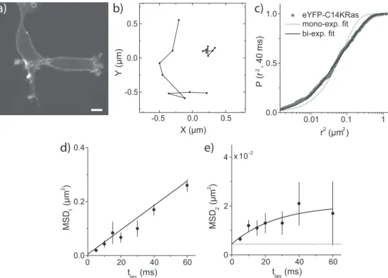
leaflets is predicted to be of importance in the transduction of cellular signals from the outside to the inside of the cell. In fig. 3a 3T3-A14 cells are shown ex-pressing eYFP-C14KRas [92]. K-Ras is generally used as a non-raft marker and comparison with the raft-marker Lck should give insights into the presence of lipid rafts.

A large number of trajectories (>2500) for eYFP-c14Kras was imaged and used for the analysis. Two of such tracjectories are shown in fig. 1.4b. Note that trajectories are relatively short because of rapid photobleaching of eYFP. From these trajectories square displacement distribution were constructed as described in section 1.2.4. The cumulative probability distribution versus the square displacement for a time lag of 40 ms is shown in fig. 1.4c. A fit of the data to eq. (1.14) clearly shows that the data cannot be described by a one-component model. The fit improves significantly when a two-one-component model is used (eq. (1.15)), while a three-component model did not improve the goodness-of-fit. Fitting the data to eq. (1.15) yielded a fast-diffusing fraction,

α=0.62±_{0.13, with MSD}₁=_0.16±_{0.04 µm}2_{and a slow-diffusing fraction with}

MSD2 =0.021±0.006 µm2. This analysis was subsequently performed for all time lags from 5 to 60 ms, and the resulting MSDs were plotted versus time lag. Figures 1.4d,e show the MSD versus time lag for the fast- and slow-diffusing fraction of the eYFP-C14KRas membrane anchor. A fit to eq. (1.8) yielded a dif-fusion constantD=1.00±0.04 µm2/s for the fast-diffusing fraction (fig. 1.4d).

For the slow-diffusing fraction the MSD-plot (fig. 1.4e) indicates that the move-ment of this fraction is confined. A fit of the data to eq. (1.10) yielded an average domain size of 219±71 nm. Studying the diffusional behavior of the Lck

an-chor in a similar manner, showed that the Lck anan-chor was not significantly slowed down as compared to the K-Ras anchor. This result does not exclude the presence of rafts in the cytoplasmic leaflet, however the size of these rafts was estimated to be smaller than 130 nm, the detection limit achieved in those experiments.

(26)

20 Introduction

a)

b)

c)

0.0 0.5 1.0

0 1 2 3

M

S

D

(μ

m

2 )

t_lag(s)

0 10 20

0.0 0.5 1.0

Asymme

try

t (s)

Directed motion

Non-directed motion

0

2 -2

0 2

-2

0

2

Z

(μ

m

)

Y (μ m) X (μ_m)

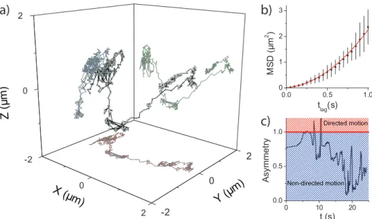
Figure 1.5:a)Trajectory of a QD loaded in to HEK293-cells obtained with a frame rate of 20 Hz for a total time of 25 s. Only one plane was imaged for each time point. In two parts of the trajectory directed transport can be clearly seen.b)MSD versus time for the first part of the trajectory where directed motion is observed. The supralinear behavior of the MSD confirms that transport takes place. A fit to the data shows that the QD has a velocity ofv=1.4±0.1 µm/s.c)Calculation of the asymmetry parameter clearly shows the two parts of the trajectory where directed motion takes place. (Asym

(27)

researchers to follow those molecules for very long time periods, only limited by the lifespan of cells. Figure 1.5 shows results of an experiment where human embryonic kidney cells (HEK293) were incubated with a solution containing 0.1 nM QDs [50]. Within two hours the QDs were internalized, after which the HEK-cells were imaged with a 3D wide-field fluorescence setup using the astigmatism method. Multiple QDs were followed simultaneously in three di-mension with high accuracy (30 nm) and at high frame rates (f = 20 Hz) without producing image stacks. In fig. 1.5a one of these trajectories is shown. What was suspected by looking at the trajectory, namely two short periods of directed transport, was confirmed unambiguously. For the first period of di-rected transport the MSD curve is plotted in fig. 1.5b. The supralinear behavior of the MSD curve confirmed that transport took place. Fitting the 3D-MSD yielded a velocity ofv=1.41±0.14 µm/s. Figure 1.5c shows that the asymmetry

parameter reliably identified the two periods of directed transport. Calculating the MSD for the initial part of the trajectory confirmed that the QD followed random diffusion during this period (D=0.015±0.001 µm2/s).

Figure 1.6 shows that current techniques can also be applied to more com-plex systems. In this case the wing imaginal disc of aDrosophila melanogaster

larva is imaged, as was introduced in section 1.1.2. After dissection the disc was placed onto the microscope and the receiving cells were imaged, in this case at a distance of 20 µm from the Dpp source. Dpp is mainly located in endo-somes with up to 250 Dpp molecules per endosome. This made it possible to track endosomes for hundreds of frames even though the Dpp is labeled with a variant of the yellow fluorescent protein. The elongated nature of the cells required making stacks consisting of 7 image planes, each separated by 1 µm. The trajectory of one endosome containing Dpp is shown in fig. 1.6a. From the projections onto the 2D planes, the 3D trajectory clearly showed up and the endosome appeared to be confined in lateral direction. Calculating the MSD curve for thex y-projection of the first 190 seconds (fig. 1.6b) clearly showed that the movement of the endosome is confined during this period. Fitting eq. (1.10) yielded an initial diffusion constantD0=1.60±0.02⋅10−3µm2/s and a lateral confinement of side lengthL =580±_{2 nm. It should be mentioned}

(28)

22 Introduction

a)

b)

c)

0 25 50 75

0.00 0.05 0.10 0.15

M

S

D

(μ

m

2 )

t_lag(s)

0 200 400

0.0 0.5

C

o

n

f

t (s)

2D Data (xy)

Confined motion Non-confined motion

-1

0

1 -1

0 1

-1 0

1

Z

(μ

m

)

Y (μ

m)

X (μ_m)

Figure 1.6: a)3D trajectory of an endosome containing Dpp molecules labeled with Venus YFP [4]. The endosome was followed for almost 600 s with a frame rate of 1 Hz. Each image stack consists of 7 image planes. b)MSD versus time-plot for the

(29)

1.3 Scope of this thesis 23

cells of ∼ 3 µm. Calculation of theConf parameter (fig. 1.6c) confirmed the observed confinement for this endosome in the first part of the trajectory.

1.2.6 Conclusion

The three examples shown clearly demonstrate that single particle tracking has become an invaluable technique to study processes in life cells and tissue. In the past two-dimensional wide-field fluorescence microscopy has become a widely used technique which has been recently complemented by several methods to provide information about the third dimension with high accu-racy. By such extension of an established methodology the range of biological questions which can be addressed is significantly broadened. In combination with superresolution techniques it will prove highly valuable and might help to lift ambiguities in present models of inter- and intra-cellular transport. We do foresee that ultimately single-molecule tracking will permit to follow intricate signalling pathways in space and time even in such complex environments as tissue. The results of such studies will by certain yield unexpected results and, more importantly, will be the solid basis for a quantitative mechanistic under-standing of cellular processes in vivo.

1.3 Scope of this thesis

This thesis reports experimental work on the Dpp morphogen gradient forma-tion, especially on the subcellular processes governing intracellular Dpp trans-port. For this purpose a 3D wide-field fluorescence microscope was developed and used in the experiments. Each chapter was written as a research article ad-dressing different aspects of the experimental method as well as specific parts of intracellular Dpp transport which were studied.

(30)

24 Introduction

internalized by living cells. Data is presented showing that the microscope is a valuable addition to existing techniques and allows for new experiments involving three-dimensional processes in live tissue.

In chapter 3 the role of the different types of endosomes in intracellulr Dpp transport is investigated. By fluorescently labeling both Dpp and Rab5 (a marker for early endosomes) the average residence time of Dpp in both early and recycling endosomes was determined experimentally. This was done by developing a new method to calculate the cross-correlation between two pop-ulations of molecules. The method, called Particle Image Cross-Correlation Spectroscopy (PICCS) has several advantages over existing methods and more reliably calculates cross-correlations between two populations of particles. With PICCS we found that early endosomes contained almost twice as much Dpp on average than other endosomes. Together with a model for intracellular transport we determined rates which are essential for a complete description of the intracellular transport of Dpp.

(31)

Bibliography

[1] Turing, A. Philos T Roy Soc B237(641):37–72 (1952). [2] Wolpert, L. J Theor Biol25(1):1–47 (1969).

[3] Lander, A. D. Cell128(2):245–56 (2007).

[4] Kicheva, A., Pantazis, P., Bollenbach, T., Kalaidzidis, Y., Bittig, T., Jülicher, F., and González-Gaitán, M. Science315(5811):521–5 (2007).

[5] Strigini, M. and Cohen, S. M. Semin Cell Dev Biol10(3):335–44 (1999). [6] Spencer, F. A., Hoffmann, F. M., and Gelbart, W. M. Cell 28(3):451–61

(1982).

[7] Nellen, D., Affolter, M., and Basler, K.Cell78(2):225–237 (1994).

[8] Letsou, A., Arora, K., Wrana, J. L., Simin, K., Twombly, V., Jamal, J., Staehling-Hampton, K., Hoffmann, F. M., Gelbart, W. M., and Massagu´e, J. Cell80(6):899–908 (1995).

[9] Lecuit, T. and Cohen, S. M. Development125(24):4901–4907 (1998). [10] del Alamo Rodr´ıguez, D., Felix, J. T., and D´ıaz-Benjumea, F. J.

Develop-mental Biology268(2):481–92 (2004).

[11] de Celis, J. F. and Barrio, R. Mech Dev91(1-2):31–41 (2000).

[12] Entchev, E., Schwabedissen, A., and Gonz´alez-Gait´an, M.Cell103(6):981– 91 (2000).

[13] Teleman, A. A. and Cohen, S. M.Cell103(6):971–80 (2000).

(32)

26 BIBLIOGRAPHY

[15] Gonz´alez-Gait´an, M. Mech Dev120(11):1265–82 (2003). [16] Basler, K. and Struhl, G. Nature368(6468):208–14 (1994). [17] Crick, F. Nature225(5231):420–2 (1970).

[18] Kerszberg, M. and Wolpert, L. J Theor Biol191(1):103–14 (1998). [19] Gonz´alez-Gait´an, M. Nat Rev Mol Cell Biol4(3):213–24 (2003).

[20] Kruse, K., Pantazis, P., Bollenbach, T., Jülicher, F., and González-Gaitán,

M. Development131(19):4843–4856 (2004).

[21] Lander, A., Nie, Q., and Wan, F. Developmental Cell2(6):785–796 (2002). [22] Anderson, C. M., Georgiou, G. N., Morrison, I. E., Stevenson, G. V., and

Cherry, R. J. Journal of Cell Science101(2):415–25 (1992).

[23] Dahan, M., L´evi, S., Luccardini, C., Rostaing, P., Riveau, B., and Triller,

A.Science302(5644):442–5 (2003).

[24] Dietrich, C., Yang, B., Fujiwara, T., Kusumi, A., and Jacobson, K.Biophys J82(1):274–84 (2002).

[25] Douglass, A. D. and Vale, R. D. Cell121(6):937–50 (2005).

[26] Harms, G. S., Cognet, L., Lommerse, P. H., Blab, G. A., Kahr, H., Gamsj¨ager, R., Spaink, H. P., Soldatov, N. M., Romanin, C., and Schmidt,

T. Biophys J 81(5):2639–46 (2001).

[27] Lommerse, P. H. M., Blab, G. A., Cognet, L., Harms, G. S., Snaar-Jagaiska, B. E., Spaink, H. P., and Schmidt, T. Biophys J 86(1):609–616 (2004). [28] Schmidt, T., Sch¨utz, G., Baumgartner, W., Gruber, H., and Schindler, H.

Proc.Natl.Acad.Sci.U.S.A.93(7):2926–2929 (1996).

(33)

BIBLIOGRAPHY 27

[30] Kubitscheck, U. Single Molecules3(5-6):267–274 (2002). [31] Goulian, M. and Simon, S. Biophys J79(4):2188–2198 (2000).

[32] K¨ohler, R. H., Schwille, P., Webb, W. W., and Hanson, M. R. Journal of

Cell Science113(22):3921–30 (2000).

[33] Sch¨utz, G., Axmann, M., Freudenthaler, S., Schindler, H., Kandror, K., Roder, J. C., and Jeromin, A. Microscopy Research and Technique

63(3):159–67 (2004).

[34] Chen, H., Yang, J., Low, P. S., and Cheng, J.-X. Biophys J94(4):1508–1520 (2008).

[35] Babcock, H. P., Chen, C., and Zhuang, X.Biophys J87(4):2749–58 (2004). [36] Seisenberger, G., Ried, M. U., Endress, T., B¨uning, H., Hallek, M., and

Br¨auchle, C. Science294(5548):1929–32 (2001).

[37] Simson, R., Sheets, E. D., and Jacobson, K.Biophys J69(3):989–93 (1995). [38] Feder, T., BrustMascher, I., Slattery, J., Baird, B., and Webb, W. W.Biophys

J70(6):2767–2773 (1996).

[39] Gelles, J., Schnapp, B. J., and Sheetz, M. Nature331(6155):450–3 (1988). [40] Kural, C., Kim, H., Syed, S., Goshima, G., Gelfand, V., and Selvin, P. R.

Science308(5727):1469–1472 (2005).

[41] Nan, X., Sims, P. A., Chen, P., and Xie, X. J.Phys.Chem.B109(51):24220– 24224 (2005).

[42] Courty, S., Luccardini, C., Bellaiche, Y., Cappello, G., and Dahan, M.

Nano Letters6(7):1491–1495 (2006).

(34)

28 BIBLIOGRAPHY

[44] Schmidt, T., Sch¨utz, G., Baumgartner, W., Gruber, H., and Schindler, H.

J.Phys.Chem.99(49):17662–17668 (1995).

[45] Zhang, B., Zerubia, J., and Olivo-Marin, J.-C.Applied Optics46(10):1819– 1829 (2007).

[46] Thompson, R., Larson, D., and Webb, W. W. Biophys J 82(5):2775–2783 (2002).

[47] Cheezum, M., Walker, W., and Guilford, W. Biophys J 81(4):2378–2388 (2001).

[48] Carter, B. C., Shubeita, G., and Gross, S. P. Phys Biol2(1):60–72 (2005). [49] Falc´on-P´erez, J. M., Nazarian, R., Sabatti, C., and Dell’Angelica, E. C.

Journal of Cell Science118(22):5243–55 (2005).

[50] Holtzer, L., Meckel, T., and Schmidt, T. Applied Physics Letters

90(5):053902 (2007).

[51] Bobroff, N. Review of Scientific Instruments57(6):1152–1157 (1986). [52] Peters, I., de Grooth, B., Schins, J., Figdor, C., and Greve, J. Review of

Scientific Instruments69(7):2762–2766 (1998).

[53] Gustafsson, M. G., Agard, D. A., and Sedat, J. W. Journal of

Microscopy-Oxford195(1):10–16 (1999).

[54] McNally, J., Karpova, T., Cooper, J., and Conchello, J.-A.Methods-A

Com-panion to Methods in Enzymology19(3):373–385 (1999).

[55] Sch¨utz, G., Axmann, M., and Schindler, H. Single Molecules2(2):69–73 (2001).

(35)

BIBLIOGRAPHY 29

[58] Levi, V., Ruan, Q., and Gratton, E. Biophys J88(4):2919–2928 (2005). [59] Lu, P. J., Sims, P. A., Oki, H., Macarthur, J. B., and Weitz, D. A. Optics

Express15(14):8702–8712 (2007).

[60] Lessard, G. A., Goodwin, P. M., and Werner, J. H. Applied Physics Letters

91(22):224106 (2007).

[61] Kao, H. and Verkman, A. Biophys J 67(3):1291–1300 (1994).

[62] Toprak, E., Balci, H., Blehm, B. H., and Selvin, P. R. Nano Letters

7(7):2043–2045 (2007).

[63] Juette, M. F., Gould, T. J., Lessard, M. D., Mlodzianoski, M. J., Nagpure, B. S., Bennett, B. T., Hess, S. T., and Bewersdorf, J.Nat.Methods5(6):527–9 (2008).

[64] Prabhat, P., Ram, S., Ward, E., and Ober, R. J.IEEE Trans.Nanobioscience

3(4):237–242 (2004).

[65] Prabhat, P., Gan, Z., Chao, J., Ram, S., Vaccaro, C., Gibbons, S., Ober, R. J., and Ward, E. S. Proc.Natl.Acad.Sci.U.S.A.104(14):5889–5894 (2007). [66] Serg´e, A., Bertaux, N., Rigneault, H., and Marguet, D. Nat.Methods

5(8):687–694 (2008).

[67] Cognet, L., Harms, G. S., Blab, G. A., Lommerse, P. H. M., and Schmidt,

T. Applied Physics Letters77(24):4052–4054 (2000).

[68] Ober, R. J., Ram, S., and Ward, E. Biophys J86(2):1185–1200 (2004). [69] Aguet, F., Ville, D. V. D., and Unser, M.Optics Express13(26):10503–10522

(2005).

[70] Betzig, E., Patterson, G. H., Sougrat, R., Lindwasser, O. W., Olenych, S., Bonifacino, J. S., Davidson, M. W., Lippincott-Schwartz, J., and Hess, H. F.

(36)

30 BIBLIOGRAPHY

[71] Hess, S. T., Girirajan, T. P. K., and Mason, M. D. Biophys J 91(11):4258– 4272 (2006).

[72] Rust, M., Bates, M., and Zhuang, X. Nat.Methods3(10):793–795 (2006). [73] Huang, B., Wang, W., Bates, M., and Zhuang, X.Science319(5864):810–3

(2008).

[74] Willig, K. I., Rizzoli, S., Westphal, V., Jahn, R., and Hell, S. W. Nature

440(7086):935–939 (2006).

[75] Geerts, H., Brabander, M. D., Nuydens, R., Geuens, S., Moeremans, M., Mey, J. D., and Hollenbeck, P. Biophys J 52(5):775–782 (1987).

[76] Ghosh, R. and Webb, W. W. Biophys J66(5):1301–1318 (1994). [77] Reinfeld, N. Mathematical Programming(1958).

[78] Veenman, C., Reinders, M., and Backer, E. Ieee T Pattern Anal23(1):54– 72 (2001).

[79] Bonneau, S., Dahan, M., and Cohen, L. Ieee T Image Process14(9):1384– 1395 (2005).

[80] Sbalzarini, I. and Koumoutsakos, P. Journal of Structural Biology

151(2):182–195 (2005).

[81] Genovesio, A., Liedl, T., Emiliani, V., Parak, W., Coppey-Moisan, M., and Olivo-Marin, J.-C. Ieee T Image Process15(5):1062–1070 (2006).

[82] Jaqaman, K., Loerke, D., Mettlen, M., Kuwata, H., Grinstein, S., Schmid, S. L., and Danuser, G. Nat.Methods5(8):695–702 (2008).

(37)

BIBLIOGRAPHY 31

[84] Coscoy, S., Huguet, E., and Amblard, F. Bull Math Biol 69(8):2467–92 (2007).

[85] Meilhac, N., Guyader, L. L., Salome, L., and Destainville, N. Physical

Review e73(1) (2006).

[86] Qian, H., Sheetz, M., and Elson, E. Biophys J60(4):910–921 (1991). [87] Huet, S., Karatekin, E., Tran, V., Fanget, I., Cribier, S., and Henry, J.

Bio-phys J91(9):3542–3559 (2006).

[88] Saxton, M.Biophys J 72(4):1744–1753 (1997).

[89] Sch¨utz, G., Schindler, H., and Schmidt, T. Biophys J 73(2):1073–1080 (1997).

[90] Deverall, M., Gindl, E., Sinner, E., Besir, H., Ruehe, J., Saxton, M., and Naumann, C. Biophys J88(3):1875–1886 (2005).

[91] Semrau, S. and Schmidt, T. Biophys J92(2):613–21 (2007).

[92] Lommerse, P. H. M., Vastenhoud, K., Pirinen, N. J., Magee, A. I., Spaink, H. P., and Schmidt, T. Biophys J 91(3):1090–7 (2006).

(38)

(39)

Chapter 2 Nanometric three-dimensional tracking of

quantum dots in living cells

1

Wide-field single-molecule fluorescence microscopy has become an established tool for the study of dynamic biological processes which occur in the plane of a cellular membrane. In the current study we have extended this technique to the three-dimensional analysis of molecular mobility. Introduc-tion of a cylindrical lens into the emission path of a microscope produced some astigmatism which was used to obtain the full three-dimensional position in-formation. The localization accuracy of fluorescent objects was calculated the-oretically and subsequently confirmed by simulations and by experiments. For further validation individual quantum dots were followed when passively dif-fusing and actively transported within life cells.

1_{This chapter is based on: L. Holtzer, T. Meckel and T. Schmidt, Nanometric}

(40)

34 3D Tracking of Quantum Dots in cells

2.1 Introduction

Wide-field single-molecule fluorescence microscopy has become an established experimental technique in the biosciences. So far its strength has mainly been exploited in two-dimensional (2D) systems: for the observation of individual molecules immobilized to substrates, and for the tracking of indi-vidual proteins in the cellular membranes [1–4]. The latter is typically carried out at video-rate allowing for simultaneous tracking of several molecules with very high lateral accuracy, far below the diffraction limit [5]. An extension of that technology to a full three-dimensional (3D) single-molecule imaging and tracking platform is highly desirable given that most biological processes take place in the 3D environment of the cell. Several methods to acquire informa-tion on the third dimension have been recently developed, i.e. using image stacks [6, 7], off-focus imaging [8] or by orbiting a focused laser beam around a particle [9]. While all these methods have shown to yield valuable informa-tion, the main disadvantage is either the imaging speed (only slow molecules can be followed) or the ability to image only one or a few molecules at a time.

(41)

2.2 Positional accuracy in three dimensions 35

2.2 Positional accuracy in three dimensions

The positional accuracy which can be achieved in lateral (x, y) and in axial (z) direction in regular imaging was estimated theoretically from the Cramer-Rao-bound assuming a Gaussian-shaped intensity distribution of a single-molecule image [12]. The Cramer-Rao bound for the position and width of the Gaussian is given bys2

µx =s 2

µy =σ

2/(₈_N_{ln 2})_and_s2

σ2 =σ4/N in whichN

is the total number of photons detected by the camera andσ the full-width-half-maximum (FWHM) of the intensity distribution. By the change of the Gaussian width with focal distance thez-position was calculated [6],

z=±zr

σ0

√

σ2₋_σ2

0 (2.1)

in whichzris the focal depth andσ0the diffraction-limited FWHM for a point-source in focus. This dependence holds for∣z∣ < 2zr ≈ 1000 nm. Error

prop-agation finally leads to an axial accuracys2

z = N1 ( z2r 2z +z2)

2

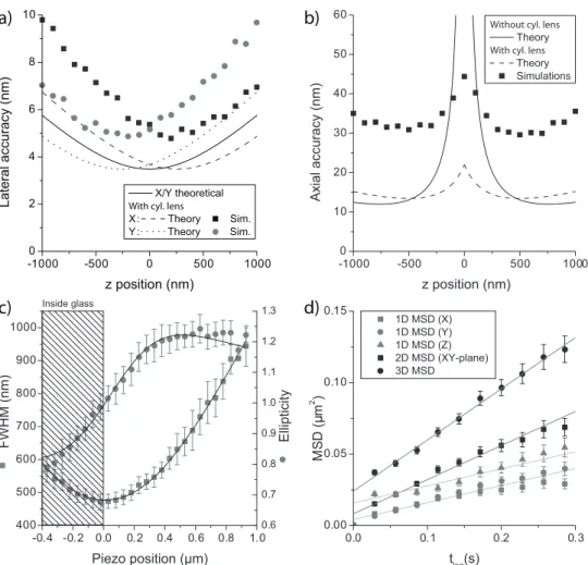
in which the errors inzr and σ0 have been neglected. Both values were determined experimen-tally with high accuracy in independent experiments. Figure 2.1a,b (solid line) shows both the lateral and the axial accuracies plotted versus the defocus po-sition. Obviously the error inzaround the focus is very large and negative and positive defocus cannot be distinguished given the symmetric dependence in

z.

Introducing a weak cylindrical lens (f =10 m) into the emission beam path results in an axial astigmatism,γ, and hence provides an easy way to increase resolution in z [11]. The intensity distribution for a point emitter including astigmatism is described by

I(x,y) =N4 ln 2

πσ2

r

e−4 ln 2[

(x−µx)2 σ2_r/є2 +

(y−µ y)2

σ2_{r є}2 ] _(2.2)

in which the ellipticityє =√σy/σx and a generalized width σr2 =

√

σ2

xσy2was

introduced. σx andσy are the FWHM of the intensity distribution inx andy

(42)

0.0 0.1 0.2 0.3

0.00 0.05 0.10 0.15 M S D (μ m 2 )

t_lag(s) 1D MSD (X) 1D MSD (Y) 1D MSD (Z) 2D MSD (XY-plane) 3D MSD

-0.4 -0.2 0.0 0.2 0.4 0.6 0.8 1.0

400 500 600 700 800 900 1000 0.6 0.7 0.8 0.9 1.0 1.1 1.2 1.3 F W H M (n m)

Piezo position (μm) Inside glass El lip ti ci ty

-1000 -500 0 500 1000

0 10 20 30 40 50 60

Without cyl. lens Theory With cyl. lens

Theory Simulations Axi a l a ccu ra cy (n m)

z position (nm)

-1000 -500 0 500 1000

0 2 4 6 8 10 X/Y theoretical With cyl. lens

X : Theory Sim. Y : Theory Sim.

L a te ra l a ccu ra cy (n m)

z position (nm)

a) b)

c) d)

Figure 2.1: Positional accuracya)in lateral (x,y) andb)in axial (z) direction for the detection of a fluorescing point object calculated according to the Cramer-Rao bound (lines), and compared to computer simulations (symbols). In the simulation each point object emitted an average of 4000 photons/frame. Each data point is an average of 1000 simulations.c)σrandєfor QDs immobilized onto a glass substrate. 10 images

(43)

2.3 Validation of the method 37

inbetween the two foci, which we define asz =0 nm. By substitutingz with

z+_γ_andz−_γ_{in eq. (2.1) to get}_σ_x_and_σ_y_{, and using the definitions for}_σ_r _and

єthe axial position is given by

z(σr,є) =⎧⎪⎪⎨⎪⎪

⎩ zr σ0 √ σ2 r

є2 −σ₀2−γ є<1

−zr

σ0

√

σ2

rє2−σ02+γ є>1

(2.3)

Analogous to the earlier treatment the Cramer-Rao bound leads to the accu-racy in each direction (see section 2.A.1 for a more detailed derivation):

s2

µx = 1

N

σ2

r/є2

8 ln 2 s 2

µy = 1

N

σ2

rє2

8 ln 2 (2.4a)

s2

z = _N1 ( √

5z2r 4(z±γ)+

√

5

4 (z±γ)) 2

є≶1 (2.4b)

As shown in fig. 2.1a,b the accuracy inz is largely increased compared to the case without cylinder lens while the accuracy in x and y is only slightly re-duced.

The theoretical strategy described above was validated by simulations. In-tensity profiles for fluorescing molecules were calculated as 2D Gaussians. Camera readout noise (σr=23 counts/pixel) and photon-counting statistics of

the detector were fully taken into account. Together with pixelation [12] this resulted in a scaling factor between simulations and theory. Additional back-ground noise was neglected. The simulations, in which the signal-to-noise ratio (SNR) was varied from 20 to 1200, confirmed that the positional accu-racy scaled with √N [12]. The positional accuracy obtained at a signal of 4000 photons/frame was 6 nm in lateral (x,y) and 30 nm in axial (z) direc-tion (fig. 2.1a,b).

2.3 Validation of the method

(44)

kW/cm2_{to obtain a SNR of 17 (275 photons/frame).} _σ

r andєwere measured

while scanning the focal plane through the sample (fig. 2.1c). From these data the focal depthzr =474±4 nm and the spot sizeσ0 =443±1 nm (z =0 nm) were determined from a fit to the given equations forσr andє. The amount of

astigmatismγ =184 nm equals that predicted. Compared to the simulations the experimental results have an increased positional accuracy. We attribute this to an overestimation ofzrin the simulations leading to an underestimated

increase of the width with defocus in the simulations. Typically 40 nm for the lateral directions (σx,σy) and 90 nm for the axial direction (σz ≈2.5σx) were

achieved, confirming that the lateral accuracy is almost unchanged while axial accuracy is largely improved.

Subsequently to the calibration experiments, QDs were dissolved to a final concentration of 0.16 nM in 15% dextran T500. The viscosity of the solution (η ≈_{300 cP at 10}○_{C) allowed us to follow the diffusional paths of the QDs for}

up to several minutes. From image sequences taken at a frequency of 35 Hz the 3D-path was reconstructed. Each trajectory was analyzed in terms of the vari-ation of the mean square displacement (MSD) with time-delay between im-ages. MSD analysis was performed for the full 3D positional information, for the projection of the trajectory onto the image plane (x y), and for the projec-tion onto each of the three spatial direcprojec-tionsx,y, andz(fig. 2.1d), respectively. As predicted for free diffusion the MSD increases linearly with time accord-ing to MSD =2nDt+∑₂_σ_n2_{, characterized by the diffusion constant}D_{of an}

n-dimensional process. The offset at zero time accounts for the positional ac-curacy in all three directions,σx,y =47 nm andσz =90 nm. Fit of the data to

this model yieldedD =0.058±_{0.003 µm}2_{/s, which is in excellent agreement}

with the free diffusion of a 22 nm-diameter particle in a solution of viscosity

η=320 cP following the Stokes-Einstein relation.

(45)

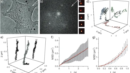
individ-2.3 Validation of the method 39 0 2 -2 0 2 -2 0 2 Z (μ m )

Y (μm )

X (μ_m)

-0.5 0.0 0.5 -1.0 -0.5 0.0 -0.5 0.0 0.5 Z ( μ m )

Y (μ m)

X (μ_m) 0 1 2 3

0.0 0.1 0.2 0.3 0.4 M S D (μ m 2)

t_lag (s)

0.0 0.2 0.4 0.6 0.8 1.0 0 1 2 3 M S D (μ m 2)

t_lag(s)

a) b) c) d)

e) f ) g)

(46)

ual QDs were analyzed (fig. 2.2d,e). From the projections onto the 2D planes, the 3D trajectory clearly showed up. The QD in fig. 2.2e shows several types of movement which can be identified by analyzing the MSDs of parts of the trajectory (fig. 2.2f,g). In the first part (fig. 2.2f) the QD was showing random diffusion (D=0.015±_{0.001 µm}2_{/s) in all dimensions. In the next part (fig. 2.2g)}

the QD shows directed motion, which was confirmed by a detailed analysis of the mobility of the QD motion in all directions. MSD analysis showed a supra-linear lag-time dependence along thex- andz-dimension for the QD. Fitting the 3D-MSD [13] yielded a velocity ofv=1.41±_{0.14 µm/s. Analysis of movement}

perpendicular to the transport did not reveal any confinement, probably be-cause the trajectory was too short (24 frames). However analysis of QDs being transported with lower velocity (example shown in fig. 2.2e) showed that the MSD perpendicular to the transport approached a constant value fortlag>3 s. Analysis showed that the QD in fig. 2.2e was confined [13] to a lateral confine-ment of side lengthL=161±_{3 nm. The size of the confinement found for this}

QD is consistent with the size of endocytic vesicles. From this we interpret that QDs were transported inside a vesicle along a cytoskeletal fiber. The velocity mentioned earlier falls within the range of speeds for a vesicle transported by molecular motors inside cells [14].

In order to verify the contribution of active intracellular transport to the observed movements, cells already containing QDs were depleted from ATP by an incubation with 20 mM NaN3and 12mM 2-Deoxy-D-glucose for 1 hour. After incubation only directed movement (fig. 2.2d,e) was abolished while ran-dom diffusion was still observed (data not shown). Hence, the supralinear de-pendence of MSD with time can clearly be attributed to ATP dependent intra-cellular processes.

2.4 Conclusion

(47)

accu-2.5 Acknowledgements 41

racy achieved approached the theoretical limit set by the Cramer-Rao bound and was 43 nm in lateral and 130 nm in axial direction inside cells at a frame rate of 167 Hz. The power of the methodology was demonstrated by detailed anal-ysis of the motion of individual QDs endocytosed by cells. The additional abil-ities of the 3D-approach was most obviously demonstrated in fig. 2.2. While a conventional 2D-approach would only have shown free diffusion and transport in a plane, the 3D-trajectory shows that the QD was transported along a tubu-lar structure that extended into the third dimension. Hence, a 2D-approach would have resulted in an incomplete interpretation of the observations.

In extrapolation of the results the fast 3D-tracking of individual fluorescent fusion proteins like the green fluorescent protein, however seems exceedingly difficult. Typically in those experiments 150 photons/frame are detected from a single molecule which would lead to an axial accuracy of σz = 120 nm at

optimal background conditions. Better results will be achieved for multiple-labeled (5-10x) objects. This will yield longer trajectories and signals of 4000 photons/frame and higher, in particular when additionally the excitation in-tensity is increased. In this way dynamic localization of e.g. vesicles inside cells at a resolution of 6 nm in lateral and 30 nm in axial direction can be easily ob-tained. Hence, the application of this fast life-cell imaging methodology to the study of e.g. vesicle trafficking or virus entry [15, 16] will prove highly valuable and might help to lift ambiguities in present models of cellular transport.

2.5 Acknowledgements

(48)

2.A

Appendix

2.A.1

Derivations

In this appendix we will show how eqs. (2.4a) and (2.4b) were derived.

The Cramer-Rao bound states that the inverse of the Fisher information matrix is the lower limit to the variance of an unbiased estimator for a statistical process. For a statistical process described by

f(x,y) = 4 ln 2

πσ2 e

−4 ln 2((x−µx)2+(y−µ y)2)

σ2 (2.5)

the estimators for µx and µy are the mean values of the distribution in either

thex ory-direction and are therefore unbiased. To calculatez the FWHMσ

is needed and to calculate the accuracy inσwe use the unbiased estimator for the variances2_:

E(s2) =_E[∑ (xi−x)2

n−1 ] =σ

2 _(2.6)

For large samplesn≈n−_{1 and therefore we assume that}_σ2_{is also an unbiased}

estimator. The Fisher information matrix is defined as

I=−E(∂U

∂θ) (2.7)

in whichU is the score function defined as the gradient of the log-likelihood function:

U(θ) =∇lnf(x,y) =∇ln4 ln 2

πσ2 −

4 ln 2((x−µ_x)2+(y−µ_y)2)

σ2 (2.8)

Taking the derivative of the log-likelihood function with respect to each unbi-ased parameter of interest yields

Uµx =

8 ln 2

σ2 (x−µx) (2.9a)

Uµy =

8 ln 2

(49)

2.A Appendix 43

Uσ2 =−

1

σ2 +

4 ln 2((x−µ_x)2+(y−µ_y)2)

σ4 (2.9c)

The Fisher information matrix is then calculated using eq. (2.7) in which

∂U

∂θ =

⎛ ⎜⎜ ⎝

−8 ln 2

σ2 0 −8 ln 2_σ4 (x −µx)

0 −8 ln 2

σ2 −8 ln 2_σ4 (y−µy)

−8 ln 2

σ4 (x−µx) −8 ln 2_σ4 (y−µy) _σ14 −

8 ln 2((x−µx)2+(y−µy)2)

σ6

⎞ ⎟⎟ ⎠

SinceE(x−µ_x) =_{0 this results in}

−E(∂U

∂θ) =

⎛ ⎜ ⎝

8 ln 2

σ2 0 0

0 8 ln 2

σ2 0

0 0 − 1

σ4

⎞ ⎟ ⎠

According to the Cramer-Rao bound the theoretical lower bound for the error (and therefore also the maximum attainable positional accuracy) in the pa-rameters µx, µy and σ2is calculated by taking the square root of the inverse

matrix:

sµx =

σ

√

8 ln 2 (2.10a)

sµy =

σ

√

8 ln 2 (2.10b)

sσ2 =σ2 (2.10c)

Using error propagationsFWHMis calculated:

sFWHM=

σ

2 (2.11)

For a process in which N photons are detected eqs. (2.10) and (2.11) should be divided by a factor √N. Previously we showed how to calculate z from eq. (2.1) and hence error propagation is used to estimate the theoretical limit to the accuracy inz:

s2

z = (

∂z

∂σ)

2

s2

σ+(

∂z

∂zr)

2

s2

zr +(

∂z

∂σ0)

2

s2

(50)

If we assume thatzr andσ0can be determined with high accuracy they can be neglected in eq. (2.12) leading to

sz=

√ (zr2

2z + z

2) 2

(2.13)

In section 2.2 it was shown that the introduction of a cylindrical lens adds the parametersγ andєto eqs. (2.1) and (2.5) and substitutes σ with σr. For our

method to work we need a small value forγ (< 300 nm). We have defined

γ as half the distance between the original position of an in-focus molecule without cylindrical lens (i.e. the focal length fo of the microscope objective,

since our microscope uses infinity-corrected optics) and the position of an in-focus molecule with cylindrical lens in the perturbed axis (so,y):

γ=sclc=

fo−so,y

2 (2.14)

in whichsclcis the so-called circle of least confusion where the image is circular (z = 0). With paraxial optics the position of the image (si,y) of a molecule at

so,y is approximated:

si,y =

1 1

ft + 1

fc − 1

d− 1 1

fo−so1,y

(2.15)

with ft the focal length of the tube lens, fc the focal length of the cylindrical

lens, fothe focal length of the objective andd the distance between objective

and cylindrical lens. Rewriting it for an in-focus molecule:

so,y =−

fo(25ftfcd−4fcd−4ftd+4ftfc)

−₂₅f_tf_cd+₂₅f_tf_cf_o+₄f_cd−₄f_cf_o+₄f_td−₄f_tf_o−₄f_tf_c (2.16)

Combining eqs. (2.14) and (2.16) allows to estimate the focal length of the cylin-drical lens needed.

(51)

2.A Appendix 45

2.A.2

Extension to image stacks

The methodology as outlined in this chapter is mainly focused on experiments in which all the particles are confined to a layer of 1.5−_{2 µm. When needed,}

for example in the experiments presented in chapters 3 and 4, the method is easily extended to a larger volume.

Recently several solutions have been proposed to image larger volumes in which for example multiple CCD cameras are used to image different planes simultaneously [17], or in which a beam splitter cube and an extra lens were used to generate a second image on the CCD camera focusing on a different plane [18].

In our experiments however we have used a different method. We placed the objective onto a piezo positioner (Physik Instrumente, Karlsruhe, Ger-many) which enabled us to move the objective in steps of 0.7-1.0 µm and hence image different focal planes in a consecutive manner, hereby generating image stacks. The advantage of this method over the two other methods is that the volume which can be imaged is in principal only limited by the working dis-tance of the objective. In the other methods the volume is limited by either the number of CCD cameras or the amount of simultaneous images that fit on the CCD chip. A clear disadvantage of our method is the imaging speed. Moving the objective from one position to the next takes around 15-20 ms and there-fore imaging of larger volumes (e.g. 7 planes) can take up to 200 ms, which includes the exposure time necessary to image each plane. In our experiments the movement of the objects of interest was low enough (see chapter 4) to as-sume that the movement of an object in a timespan of 50 ms (needed to image two planes) is smaller than the positional accuracy of our system.

(52)

Subcellular processes in morphogen gradient formation studied with 3D-tracking fluorescence microscopy

Subcellular processes in morphogen

gradient formation studied with

3D-tracking fluorescence microscopy

Subcellular processes in morphogen

gradient formation studied with

3D-tracking fluorescence microscopy

Proefschrift

Laurentius Henricus Franciscus Maria Holtzer

Contents

Chapter 1

Introduction

1.1

The morphogen gradient

1.1.1

Morphogens

1.1.2

Dpp

1.1.3

Morphogen spreading

1.2

Particle tracking in cells and tissue

1.2.1

Single-molecule and single-particle localization

1.2.2

Positional accuracy

1.2.3

Tracking

1.2.4

Trajectory analysis

1.2.5

Applications

a)

b)

c)

a)

b)

c)

1.2.6

Conclusion

1.3

Scope of this thesis

Bibliography

Chapter 2

Nanometric three-dimensional tracking of

quantum dots in living cells

2.1

Introduction

2.2

Positional accuracy in three dimensions

2.3

Validation of the method

2.4

Conclusion

2.5

Acknowledgements

2.A

Appendix

2.A.1

Derivations

2.A.2

Extension to image stacks