Approximate Bayesian computing for spatial extremes

(1)

Approximate Bayesian Computing for Spatial

Extremes

Robert J. Erhardt

A dissertation submitted to the faculty of the University of North Carolina at Chapel Hill in partial fulfillment of the requirements for the degree of Doctor of Philosophy in the Department of Statistics and Operations Research.

Chapel Hill 2012

Approved by:

Richard L. Smith, Advisor

Lawrence Band, Reader

Joseph Ibrahim, Reader

Chuanshu Ji, Reader

(2)

(3)

ABSTRACT

ROBERT J. ERHARDT: Approximate Bayesian Computing for Spatial Extremes.

(Under the direction of Richard L. Smith.)

Statistical analysis of max-stable processes used to model spatial extremes has been lim-ited by the difficulty in calculating the joint likelihood function. This precludes all standard likelihood-based approaches, including Bayesian approaches. Here we present a Bayesian approach through the use of approximate Bayesian computing. This circumvents the need for a joint likelihood function and instead relies on simulations from the (unavailable) like-lihood. This method is compared with an alternative approach based on the composite likelihood. When estimating the spatial dependence of extremes, we demonstrate that ap-proximate Bayesian computing can provide estimates with a lower mean square error than the composite likelihood approach, though at an appreciably higher computational cost.

As this approach very naturally incorporates parameter uncertainty into predictions, it is well suited for use in pricing weather derivatives to manage environmental risks. We discuss the construction and pricing of such weather derivatives. The method described utilizes results from spatial statistics and extreme value theory to first model extremes in the weather as a max-stable process, and then use these models to simulate payments for a general collection of weather derivatives. These simulations capture the spatial dependence of payments. Incorporating results from catastrophe ratemaking, we show how this method can be used to compute risk loads and premiums for weather derivatives which are renewal-additive.

(4)

Acknowledgments

To Mar and Nolan with thanks to Richard

(5)

List of Figures

2.1 Standard unit-Fr´echet, Weibull, and Gumbel density functions. . . 6

2.2 A few correlation functions for Gaussian processes. . . 13

2.3 Gaussian extreme process. . . 16

2.4 Whittle-Mat´ern correlation function for isotropic and non-isotropic cases. . 17

2.5 Extremal Gaussian process. . . 18

2.6 Brown-Resnick process. . . 19

3.1 Madogram. . . 35

3.2 Example of triplets and computation of distance. . . 38

3.3 Span of Models in ABC Simulation Study. . . 42

4.1 Example of AABC Method. . . 48

4.2 Example of k-means++ clustering. . . 52

4.3 Example of Ward’s clustering. . . 53

4.4 Run times for clustering methods. . . 54

4.5 Mean square error and K. . . 55

4.6 Average mean square error and K. . . 56

4.7 The number of unique k-tuples in a data set with D locations. . . 57

4.8 Mean square error and threshold . . . 59

4.9 Impact of uniform priors on the correlation functions. . . 61

4.10 Impact of non-uniform priors on the correlation functions. . . 62

5.1 Phoenix airport temperature example. . . 73

5.2 Diagnostics from Phoenix airport example. . . 74

(8)

5.4 Estimates of risk measures for hypothetical weather derivative. . . 80

5.5 Estimating the marginal variance of a weather derivative. . . 83

6.1 Locations of Midwest temperature data. . . 89

6.2 Empirical estimates of risk measures for Midwest temperature example. . . 91

6.3 AABC Posterior in Midwest temperature example. . . 96

6.4 Empirical estimates of risk measures for Midwest temperature example. . . 97

6.5 Locations for Texas cotton example. . . 99

6.6 Estimated GEV parameters for the Texas cotton example. . . 100

6.7 Kriged GEV parameters for the Texas cotton example. . . 100

6.8 ABC Posterior for Texas cotton example. . . 102

(9)

List of Tables

3.1 Mean square error from ABC-REJ simulations. . . 42

4.1 Mean square error from AABC simulations. . . 49

4.2 Permutations in triplet distance calculation. . . 58

4.3 Mean square error of AABC and asymptotics. . . 63

4.4 Mean square error of AABC and thresholds, D=20. . . 63

4.5 Mean square error of AABC and thresholds, D=40. . . 63

5.1 Moments for Phoenix airport example (1). . . 75

5.5 Simulated payments of a hypothetical weather derivative. . . 79

5.6 Mean absolute error of marginal variance estimation. . . 82

6.1 Payments for Midwest temperature example, MCLE. . . 90

6.2 Payments for the Midwest temperature example, AABC. . . 96

(10)

1 Introduction

Modeling of spatial extremes is motivated by the need to model and predict environmental

extreme events such as hurricanes, floods, droughts, heat waves, and other high impact

events. Though the data have a natural spatial domain, standard spatial statistics methods

may fail to accurately model extremes. Models specifically designed for extremes are better

suited. The urgency of focusing on extremes is increased when one considers the potential

influence of climate change on the probability of such high impact events. We consider

point referenced data, usually taken as daily or hourly measurements yt,d at locations

d= 1, ..., D for time points t= 1, ..., T. When modeling extremes, as a first step one takes

block maxima over some temporal block (usually one year) and obtains block maxima

datayi,d where iis the block. In an environmental setting, for example, the data might be

annual maxima at each of D locations.

For a single location, univariate extreme value theory provides a full range of tools to

analyze the data. This theory is well developed and documented (Coles, 2001; de Haan and

Ferreira, 2006; Embrechts, et. al., 1999; Resnick, 1987, 2007). When one considers several

locations at once, multivariate extreme value theory is a natural extension. Multivariate

models often work well for lower dimensions, but if the data have a natural spatial domain

(11)

is to fit these block maxima data to a spatial process model so that the spatial dependence

may be estimated. One promising class of models are max-stable processes. These arise as

the limiting distribution of the maxima of independent and identically distributed random

fields. A number of max-stable process models have been described (Schlather, 2002;

Kabluchko et. al., 2009) and one unpublished model was described by Smith in 1990. The

statistical analysis of these models is limited by the unavailability of the joint likelihood

function. However, the bivariate distributions are available in closed-form. This allows one

to write down the pairwise log-likelihood, which is the sum (taken over all unique pairs

of locations) of all bivariate log-likelihoods, and is thus also a composite log-likelihood.

Numerical maximization of the composite likelihood yields estimates of the parameters

which are consistent and asymptotically normal (Padoan et. al., 2010; Lindsay, 1988).

Maximum composite likelihood estimation has been the only method so far for analyzing

max-stable processes which is widely applicable, implemented computationally (R package

SpatialExtremes), and for which a viable asymptotic theory exists.

In this dissertation we develop a Bayesian alternative for analyzing the dependence

of spatial extremes. It circumvents the need for the joint likelihood, and instead relies

only on simulations. This approach, termed approximate Bayesian computing, has been

successfully applied in many areas, including extreme values (Bortot et. al., 2007). We

show three implementations of the approximate Bayesian computing approach for analyzing

spatial extremes. The first two rely on the bivariate distribution function, and like the

composite likelihood approach they consider the spatial dependence through all unique

pairs of locations. The third and most successful approach extends beyond pairs, and is

able to consider higher orderk-tuples fork_>3. This feature is an important benefit of the

approximate Bayesian computing approach over all pairwise approaches. We show that the

approximate Bayesian computing method can result in a lower mean square error compared

(12)

We also discuss how this Bayesian approach naturally incorporates parameter uncertainty

into predictions, which is a central task in the field of extremes.

The method is computationally intensive, but open to a number of computational

en-hancements as well. The simplest implementation based on rejection sampling can be done

in parallel, and we demonstrate this. A more efficient implementation takes advantage of

adaptive computing, in which the sampler targets regions of the parameter space which

have shown greater promise. Not only does this approach reduce the computational cost,

but it also makes the choice of prior distribution an easier one. We advocate choosing

minimally informative, independent uniform priors on the natural parameters space Φ,

and show how adaptive approximate Bayesian computing can smoothly move from these

minimally informative priors to the target posterior distribution at a reasonable

compu-tational cost. Furthermore, compucompu-tational considerations of various enhancements to the

algorithm are discussed.

We connect the statistical methodology with an application of rising interest in the

insurance industry - how to price weather derivatives for use as a risk management tool.

Weather derivatives are contingent contracts whose payments are determined by the

dif-ference between some underlying weather measurement and a pre-specified strike value.

They provide a useful risk management tool for any party facing weather risk. They also

provide investments which are often uncorrelated with more traditional financial

instru-ments, allowing investors to diversify. The first weather derivative was developed in 1996,

and by 1999 derivatives and their options were being traded on the Chicago Mercantile

Exchange (Kunreuther and Michel-Kerjan, 2009).

Finally, we demonstrate the use of max-stable processes for pricing weather derivatives

for extremes, both from a frequentist and Bayesian perspective. The Bayesian approach has

the added advantage of naturally incorporating parameter uncertainty into estimated risk

(13)

application, we demonstrate how the approach can be used to extrapolate models from

regions of data to regions of interest, and serve as a rare event simulator. These simulators

(14)

2 Extremes

2.1 Univariate and Multivariate Extremes

Let Y1, ..., Yn be univariate i.i.d. replicates from some distribution function F, and define

Mn= max(Y1, ..., Yn) as the maximum of then random variables. The distribution of Mn

can be obtained exactly assumingF is known. In practice, then one could estimateF from

all of the data Y1, ..., Yn and estimate the distribution of Mn as P(Mn 6z) = Fn(z), but

this approach has two drawbacks. The first is that even minor discrepancies in estimating

F result in large discrepancies in Fn_{, particularly in the tails of} _F_{. Put another way, why}

should we expect a model which fits the bulk of data to also be a good fit in the tails? A

second drawback is that in the limit asn → ∞,Fn _{does not converge to a non-degenerate}

distribution.

Instead, we model renormalized maxima Mn−bn

an for sequences an > 0 and bn. If there

exist sequences an >0 and bn such that

lim

n→∞P

Mn−bn

an 6

z

→G(z)

(15)

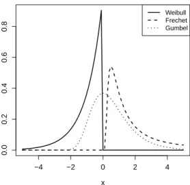
−4 −2 0 2 4 0.0 0.2 0.4 0.6 0.8 x Weibull Frechet Gumbel

Figure 2.1: Standard unit-Fr´echet, Weibull, and Gumbel density functions. These are obtained by setting a= 1, b= 0, andα= 1 in equations (2.1), (2.2), and (2.3).

following families:

I :G(z) = exp

−exp

−

z−b a

, −∞< z <∞ (2.1)

II :G(z) =

  

 

0, z ₆b

exp{− z−b a

−α

}, z > b

(2.2)

III :G(z) =

  

 

exp−

− z−b a

α

, z < b

1, z _>b,

(2.3)

with parametersa >0,b, andα >0 for types II and III. This result is known as the

Three-Types Theorem (Fisher and Tippett, 1928), and the three families are Gumbel, Fr´echet, and

Weibull, respectively. The Fr´echet case corresponds to a heavy tailed distribution, Gumbel

is intermediate, and Weibull has a bounded upper limit. Standard density functions for

the three families are shown in Figure 2.1.

(16)

must choose one of the families, and then all subsequent inference assumes the choice to be

correct. To avoid this, the three families are often written as a singleGeneralized Extreme

Value (GEV) family, with distribution function

G(z) = exp

"

−

1 +ξz−µ σ

−1/ξ

+

#

.

Here a+ = max(a,0), and µ, σ, and ξ are the location, scale, and shape parameters,

respectively (Coles, 2001; Gnedenko, 1943). The sign of the shape parameter ξ

corre-sponds to the three classical extreme values distributions: ξ > 0 is Fr´echet with support

z ∈[µ−σ/ξ,+∞),ξ <0 is Weibull with supportz ∈(−∞, µ−σ/ξ], and ξ→0 is Gumbel with support z ∈ (−∞,+∞). When using this model, one allows the estimate of ξ to guide which of the three types is selected.

The Generalized Extreme Value distribution G has the property of max-stability,

un-derstood as follows: ifY1, ..., Ynare i.i.d. fromG, then max(Y1, ..., Yn) also has distribution

G, meaning

Gn(Anz+Bn) = G(z)

for appropriate sequencesAn >0 and Bn. In fact, a distribution is max-stable if and only

if it is a member of the GEV family (Leadbetter et. al., 1983). If block maxima are taken

over a block size large enough to allow the GEV to be a valid approximation, then if one

further increased the block size (from monthly to annual maxima, for example) the GEV

model would still hold, with only a change in the three parameters. While these results

for the GEV family assume i.i.d. data, this assumption can be relaxed and the limiting

distribution still holds so long as certain mixing conditions are satisfied (Leadbetter et.

al., 1983).

(17)

function

P(Z ₆z) = exp

−1

z

.

The simplicity of the distribution function is helpful when one considers multivariate and

ultimately spatial extremes. Any member of the GEV family may be transformed to have

unit-Fr´echet margins as follows: if Z has a GEV distribution, and a new variable U is

defined as

U =

1 +ξZ−µ σ

1/ξ

, (2.4)

then U has unit-Fr´echet margins. This transformation assumes that the parameters are

known. If the parameters are unknown, they may first be estimated and then the

transfor-mation toU is taken. Ultimately, when we have extreme values data in a spatial setting, the

first step will be to transform data at each location to unit-Fr´echet by fitting all marginal

distributions. Then we will proceed to analyze the spatial dependence among sites once

every location has been transformed. Thus, for the remainder of this dissertation there is

no loss of generality when one assumes unit-Fr´echet margins.

The GEV model can be fit to observed data using maximum likelihood estimation.

Call the parameter vector φ. This parameter can be as simple as three fixed parameters,

as φ = (µ, σ, ξ). Alternatively, one can model the GEV parameters using temporal or

spatial covariates. A few examples include µ = µ1 + µ2 · t, where t is time, or σ = σ1+σ2·lat+σ3·lon+σ4·elev, which considers effects of latitude, longitude, and elevation

on the scale parameter. No matter the structure of the parameter φ, define the density

function g(z;φ) = _dzdG(z;φ). Then, the maximum likelihood estimate of φ is

ˆ

φM LE = argmaxφ

Y

i

g(z |φ) (2.5)

This maximization is often done numerically, and has been implemented in a number of

(18)

in the package evd. The density function for the fitted model is obtained by plugging in

the maximum likelihood estimate as g(z; ˆφM LE).

We may extend this approach to handle multivariate extremes. Let (Xi1, ..., XiD),

i= 1, ..., nbe a D−dimensional random vector and let Mn= (Mn1, ..., MnD) be the vector

of componentwise maxima, where Mnd = max(X1d, ..., Xnd) for d = 1, ..., D. It is worth

noting that Mn will not appear in the data record unless the occurrence times of each

element’s block maximum happen to coincide. In a spatial context, this vectorMn might

refer to the annual maxima of some variable at D locations. A non-degenerate limit for

Mn exists if there exist sequences and >0 andbnd, d= 1, ..., D such that

lim

n→∞P

Mn1−bn1 an1

6z1, ...,

MnD−bnD anD

6zD

=G(z1, ..., zD).

Then G is a multivariate extreme value distribution (MEVD), and is max-stable if there

exist sequences And >0,Bnd,d= 1, ..., D such that, for any n >1

Gn(z1, ..., zD) =G(An1z1+Bn1, ..., AnDzD +BnD).

The marginal distributions of a multivariate extreme value distribution are all

necessar-ily GEV distributions. Thus, for each margin one can define a transformation like the one

shown in equation (2.4) with parameter (µd, σd, ξd) and transform to unit-Fr´echet. Since

all GEV distributions can be transformed into unit-Fr´echet, all MEVD can be transformed

into multivariate unit-Fr´echet, and thus we may assume, without loss of generality, that all

MEVD have unit Fr´echet margins. This is because the domain of attraction condition is

preserved under monotone transformations of the marginal distributions (Resnick, 1987).

Thus for D fixed locations, the joint distribution function can be written as

(19)

whereV(z1, ..., zD) is the exponent measure first described by Pickands (1981). This

func-tion takes the form

V(z) = D·

Z

∆D

max

d=1,...,D

wd zd

H(dw) (2.7)

where ∆D =w∈RD+ |w1+...+wD = 1 is theD−1 dimensional simplex, and the angular

(or spectral) measure H is a probability measure on ∆D which determines the dependence

structure of the random vector. Due to the common marginal distributions,Hhas moment

conditions R_∆

DwdH(w) = 1/D for d= 1, ..., D. Max-stability implies that for all N,

P(Z1 6z1, ..., ZD 6zD)N = exp(−N ·V(z1, ..., zD)) = exp(−V(z1/N, ..., zD/N))

with the final equality following from the homogeneity property of the exponent measure.

The measure also satisfies two bounds: if all locations are independent, V(z1, ..., zD) =

1/z1+...+ 1/zD; if all locations are totally dependent, V(z1, ..., zD) = max(1/z1, ...,1/zD).

Thus, we always have max(1/z1, ...,1/zD)6V(z1, ..., zD)61/z1+...+ 1/zD.

There are two challenges to working with the spectral representation of the joint

distri-bution function shown in equation (2.6). First, even if we assume that a closed form for the

exponent measure can be found by solving equation (2.7), the joint density function

un-dergoes a combinatorial explosion as the dimension D increases. Differentiating exp(−V) with respect to the values z1, ..., zD leads to a rapid growth in terms:

• −V1exp(−V) (first partial derivative)

• (V1V2−V12) exp(−V) (second partial derivative)

• (−V1V2V3+V12V3+V13V2+V23V1−V123) exp(−V) (third partial derivative)

• ...

whereVi is the partial derivative of V with respect to zi. Thus even if a reasonable choice

(20)

function, which may be difficult to maximize. More common, though, is the situation

where closed-form expressions for the exponent measure cannot be obtained by solving

equation (2.7). This holds for all of the widely used max-stable process models, resulting

in an unavailable joint likelihood function.

2.2 Background on Spatial Statistics

The basic object in spatial statistics is a stochastic process Y(x), x ∈ X where X is a subset of _Rp_{, usually with} _p_{= 2. Let}

δ(x) = _E(Y(x)), x∈X

be the mean of the process defined for all of X, and assume that the variance of Y(x)

exists everywhere in X. Then the process can be rewritten as

Y(x) = δ(x) +e(x)

where δ(x) is the non-random mean function and e(x) is a zero-mean stochastic process.

One often models the mean of the process with covariates, i.e. δ(x) = W(x)T_β_{, where}

W(x) are covariates and β is a vector of regression covariates.

The process is said to be Gaussian if for any D _> 1 and locations x1, ..., xD, the

vector (e(x1), ..., e(xD)) has a mean-zero multivariate normal distribution, which in turn

implies that the vector (Y(x1), ..., Y(xD)) has a multivariate normal distribution with

mean (δ(x1), ..., δ(xD)). The process is strictly stationary if the joint distribution of

(21)

points x1, ..., xD. For a Gaussian process, strict stationarity implies

Cov(Y(x1), Y(x2)) =C(x1−x2) for all x1, x2 ∈X.

That is, the covariance of the process at any two locations is some function C which

depends only on the separation vector between points, and not the particular locations.

This is also called second-order stationarity. Next, we define the variogram through the

relation

Var(Y(x1)−Y(x2)) = 2γ(x1 −x2)

where the quantity 2γis the variogram, andγis thesemi-variogram. Under the assumption

of strict (or second-order) stationarity,

γ(h) =C(0)−C(h) = C(0)(1−ρ(h))

where ρ(h) is the correlation between two locations separated by vector h. Further, if

we have γ(h) = γ(||h||) for all h ∈ X, meaning if the semi-variogram only depends on

h through its length ||h||, then the process is isotropic. The correlation function ρ(h) is then usually chosen from one of the valid families of correlation functions for Gaussian

processes. A few common choices of isotropic, stationary correlation functions are the

Whittle-Mat´ern,

ρ(h) = c1

21−ν

Γ(ν)

h c2

ν

Kν

h c2

, 0₆c1 61, c2 >0, ν >0, (2.8)

Cauchy,

ρ(h) =c1

(

1 +

h c2

2)−ν

(22)

0 2 4 6 8 10 0.0 0.2 0.4 0.6 0.8 1.0 Whittle−Matern h range=1 range=3 range=5

0 2 4 6 8 10

0.0 0.2 0.4 0.6 0.8 1.0 Cauchy h range=1 range=3 range=5

0 2 4 6 8 10

0.0 0.2 0.4 0.6 0.8 1.0 Power Exponential h range=1 range=3 range=5

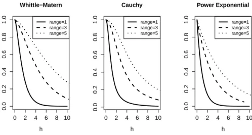
Figure 2.2: A few correlation functions for Gaussian processes. Left panel: Whittle-Mat´ern. Center panel: Cauchy. Right panel: Power Exponential. Each function is shown with nuggetc1 = 1, smoothν = 1, and rangec2= 1,3,and 5, using equations (2.8), (2.9),

and (2.10).

and powered exponential

ρ(h) =c1exp

− h c2 ν

0₆c1 61, c2 >0,0< ν 62, (2.10)

wherec1, c2 and νare the nugget, range, and smooth parameters, Γ is the gamma function

and Kν is the modified Bessel function of the third kind with order ν. A few sample

correlation functions are shown in Figure 2.2.

It is common to fix the nugget as c1 = 1, which forces ρ(h) → c1 = 1 as h → 0.

This is a reasonable assumption for many environmental processes, and we make this

assumption throughout this dissertation and do not attempt to model the nugget. We

should clarify, though, that the theory and methods described in this dissertation would

apply even if c1 6= 1, and so this restriction is not required. Throughout the remainder

of this dissertation, the unknown spatial dependence parameter is called φ = (c2, ν), and

unless stated otherwise we will assume spatial extremes models which are both stationary

(23)

2.3 Spatial Extremes and Max-stable Processes

Max-stable processes arise as the infinite dimensional generalization of multivariate extreme

value theory. Let Z(x), x ∈ X ⊆ _Rp _{be a spatial process. If for all} _n _> _{1, there exists}

sequencesan(x), bn(x), x∈X such that for anyx1, ..., xD ∈X,

Pn

Z(xd)−bn(xd) an(xd) 6

z(xd), d= 1, ..., D

→Gx1,...,xD(z(x1), ..., z(xD))

thenGx1,...,xD is a multivariate extreme value distribution. If the above holds for all possible

subsets x1, ..., xD ∈X for any D>1, then the process is max-stable.

The definition of a max-stable process as the infinite dimensional generalization of the

multivariate extreme value distribution gives a well-defined model, but not an obvious way

of constructing such a process. A conceptual construction with spectral representation was

given by de Haan (de Haan, 1984; de Haan and Ferreira, 2006). LetY(x) be a non-negative

stationary process on _Rp such that _E(Y(x)) = 1 at eachx. Let Π be a Poisson process on

R+ with intensity s−2ds. If Yi(x) are independent replicates of Y(x), then

Z(x) = maxsi·Yi(x), x∈X

is a stationary max-stable process with unit Fr´echet margins . From this, the joint

distri-bution may be represented as

P(Z(x)₆z(x), x∈X) = exp

−_E

sup

x∈X

Y(x)

z(x)

,

where _Ehsup_x_∈_X Y_z₍(_xx₎)i is the exponent measure V(z) shown in equation (2.6). Varying

the choice of the process Y(x) gives different max-stable processes. Smith (unpublished

manuscript, 1990) constructed a process known as the Gaussian extreme value process. Let

(24)

s−2_dsdx_{. Take} _f₍_{x, x}

i) to be the multivariate Gaussian density function,

f(x, xi) = (2π)−p/2|Σ|−1/2exp

−1

2(x−xi)

T_Σ−1₍_x₋_x

i)

.

ThenZ(x) = maxisif(x, xi) is a max-stable process with unit-Fr´echet margins. Smith also

introduced the “rainfall-storms” interpretation: think of_Rp _{as the space of storm centers,}

si as the magnitude of the ith storm, and f(x, xi) as the shape of the storm centered

at position xi. The maximum of independent storms at each location x is taken to be

the max-stable process. With this framework, the bivariate distribution function of the

max-stable processZ can be written as

P(Z1 6z1, Z2 6z2) = exp

−1 z1 Φ a 2 + 1 alog z2 z1 − 1 z2 Φ a 2 + 1 alog z1 z2 (2.11)

where Φ is the standard normal distribution function,a2 _{= (}_x

1−x2)TΣ−1(x1−x2), and Σ

is the covariance matrix of f with covariance σ12 and standard deviations σ1 and σ2. The

dependence parametera represents a transformed distance between the two sites, and the

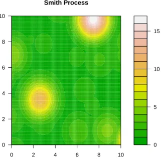
limitsa →0 anda→ ∞correspond to perfect dependence and independence, respectively. Figure 2.3 shows one realization of this process.

Schlather (2002) introduced a more flexible set of models for max-stable processes by

taking Y(x) to be any stationary Gaussian process (and not just a multivariate normal

density) with finite expectation. He considered a stationary Gaussian process Y on _Rp

with correlation function ρ(·) and finite mean µ = _Emax(0, Y(x)) ∈ (0,∞). Let si be a

Poisson process on (0,∞) with intensity measure µ−1_s−2_ds_{. Then}

Z(x) = max

i simax(0, Yi(x))

(25)

0 5 10 15

0 2 4 6 8 10

Smith Process

Figure 2.3: Gaussian extreme process with parameters (σ1=σ2 = 9/8, σ12= 0)

.

function is

P(Z1 6z1, Z2 6z2) = exp

−1 2

1

z1

+ 1

z2

1 +

r

1−2(ρ(h) + 1) z1z2 (z1+z2)2

(2.12)

whereρ(h) is the correlation of the underlying Gaussian processY andh=||x1−x2||. The

correlation is chosen from one of the valid families of correlations for Gaussian processes,

such as those shown in equations (2.8), (2.9) and (2.10). Following the rainfall-storms

interpretation from Smith, the Schlather model takes maxima over a series of storms with

the same dependence structure, but their realizations vary stochastically. This allows

storms to have random shapes, unlike the deterministic multivariate normal shapes of

the Smith model. Figure 2.5 shows one realization of a process with the Whittle-Mat´ern

correlation function. This is generally considered a more realistic representation of an

(26)

0.1

0.2 0.3

0.4

0.5

0.6

0.7

0.8

−40 −20 0 20 40

−40

−20

0

20

40

0.1 0.1

0.2

0.3 0.4

0.5 0.6

0.7 0.8

0.9

−40 −20 0 20 40

−40

−20

0

20

40

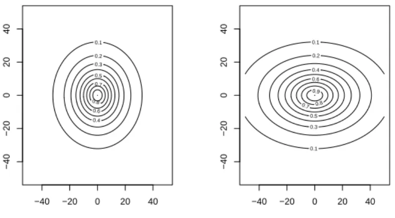
Figure 2.4: Whittle-Mat´ern correlation function with nugget=1, range=10, and smooth=1 for the isotropic case (left panel) and non-isotropic case (right panel).

focus on the Schlather model exclusively, but the methodology can be applied to any

parametrically specified max-stable process from which realizations can be simulated.

Although the correlation functions ρ(·) shown above all assume isotropy, the Schlather model does not explicitly require this assumption. Ribatet (2011) gives a convenient

method for extending the approach to non-isotropic data through a space warping

ar-gument. Given a valid, isotropic correlation function ρ(·), one may define an elliptical correlation function ρe(∆x) = ρ(

√

∆xT_A_∆_x_{) where ∆}_x _{is the vector between two}

loca-tions, and the matrix A handles the space-warping into an elliptical measure of distance

(and would contain additional dependence parameters). An example of an elliptical

corre-lation function in _R2 _{is shown in Figure 2.4.}

One drawback to the Schlather model is that it cannot attain the case of independence

for extremes as distance h → ∞. To overcome this problem, the process Y(x) can be restricted to a random set B, i.e.,

Z(x) = max

(27)

0 1 2 3 4 5 6 7

0 2 4 6 8 10

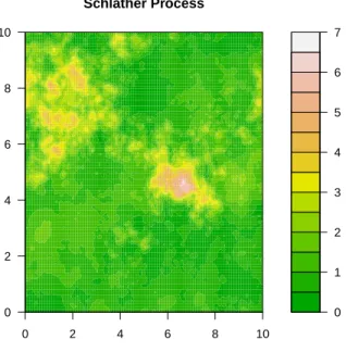
Schlather Process

Figure 2.5: Extremal Gaussian process with Whittle-Mat´ern correlation with nugget c1 = 1,

range c2= 3, and smooth ν= 1.

whereIB is the indicator function for a random setB ⊂X andxi. IfYi is again a Gaussian

process, then the bivariate distribution function can be written as

exp

−

1

z1

+ 1

z2

1− α(h) 2

1−

r

1−2(ρ(h) + 1) z1z2 (z1+z2)2

where α(h) = _E|B ∩(h+B)|/_E(|B|) ∈ [0,1]. This modification permits independent ex-tremes in the limit ash→ ∞. One possible choice forB is a disc of radiusr, which implies

α(h) = {1− |h|/(2r)}+, which equals 0 when |h| > 2r. Choices for B were explored by

Davison and Gholamrezaee (2010).

Kabluchko et. al. (2009) proposed an alternative specification for theY(·) processes, one with a weaker assumption than second-order stationarity. LetY(x) = exp{s(x)−1₂σ2(x)}

wheres(x) is a Gaussian process with stationary increments andσ2(x) = V ar{(x)}. Then

(28)

0 2 4 6 8 10

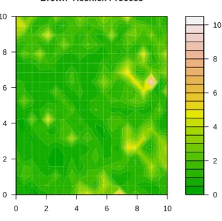
0 2 4 6 8 10 Brown−Resnick Process

Figure 2.6: Brown-Resnick process with Whittle-Mat´ern correlation with nugget c1 = 1, range c2 = 3, and smoothν = 0.5.

to unit Fr´echet margins is the same as the Smith model where the dependence parameter

a2 =γ(h), andγ(·) is the variogram of (·). The closed form of the bivariate distributions for the Brown-Resnick process associated to the variogramγ are given by

P {Z(x1)6z1, Z(x2)6z2}

= exp ( − 1 z1 Φ p

γ(h)

2 +

1

p

γ(h)log

z2 z1 ! − 1 z2 Φ p

γ(h)

2 +

1

p

γ(h)log

z1 z2

!)

(2.13)

where Φ is the standard normal distribution function and h is the Euclidean distance

between locationx1 and x2. A realization is shown in Figure 2.6.

Each of the max-stable processes introduced above share some common features. First,

they are all well defined, and can all be simulated using the point process approach outlined

by de Haan (1984) with different choices of stochastic process Y(x). Additional results on

(29)

(2012), and Dombry et. al. (2012). Second, all finite dimensional distributions follow a

MEVD, and we know that all marginal distributions at all locations x1, ..., xD follow a

GEV distribution, all of which can thus be transformed to unit-Fr´echet by the one-to-one

transformations

Y(xd) =

1 +ξ(xd)

Z(xd)−µ(xd) σ(xd)

1/ξ(xd) .

Without loss of generality then, one may assume that a max-stable process has unit-Fr´echet

margins. Finally, bivariate distribution functions can be written out as shown in equations

(2.11), (2.12), and (2.13), and in each case the spatial dependence parameters Σ, ρ(·), or γ(·) appear in these bivariate functions. To generalize and simplify notation for the remainder of this dissertation, we will call the generic dependence parameter φ.

2.4 The Extremal Coefficient

Let Z(x) be a stationary, isotropic max-stable random field with unit-Fr´echet margins.

As shown in equation (2.6), for D fixed locations the joint distribution function for a

max-stable process can be written as

P(Z(x1)6z1, ..., Z(xD)6zD) = exp{−V(z1, ..., zD)}

where V(z1, ..., zD) is the exponent measure first described by Pickands (1981).

Max-stability implies that for all N,

P(Z1 6z1, ..., ZD 6zD)N = exp{−N V(z1, ..., zD)}= exp{−V(z1/N, ..., zD/N)}.

The final equality arises as a consequence of the homogeneity property of the exponent

measure. For each of the studied classes of max-stable processes, for D ₆ 2 locations

(30)

to this is for the Smith model, where the trivariate distribution can be written in closed

form if X ⊂ _R2_{, explored in Genton et. al. (2011). However, for the other max-stable}

processes only univariate and bivariate distributions are available in closed-form). If we

further consider the joint distribution ofD locations evaluated at the same valuez, we get

P(Z(x1)6z, ..., Z(xD)6z) = exp

−θ(x1, ..., xD)

z

where θ(x1, ..., xD) =V(1, ...,1) is the extremal coefficient for the D locations. Since the

bounds on the extremal coefficientV(z1, ..., zD) are 1/z1+...+1/zDand max(1/z1, ...,1/zD),

bounds on the extremal coefficient areDand 1, respectively, with a value ofD

correspond-ing to complete independence and a value of 1 correspondcorrespond-ing to complete dependence. The

value can be thought of as the number of effectively independent locations among the D

under consideration.

Many results are available for the pairwise extremal coefficient, which arises when

considering any pair of locations,

P(Z(x1)6z, Z(x2)6z) = exp

−θ(x1, x2)

z

Since the bivariate distribution functions are available in closed form equation (2.12) for

the Schlather process, one may write out the pairwise extremal coefficients explicitly as

θ(h) = 1 +

1−ρ(h;φ) 2

1/2

(2.14)

where h = ||x1−x2||. One may estimate the pairwise extremal coefficients directly from

the data, and then through those estimates obtain an estimate ofρ(·). Smith (Smith 1990, unpublished manuscript) and Coles and Dixon (1999) proposed an estimate of the pairwise

(31)

unit-Fr´echet. This means that 1/Z(·) is unit exponential, and 1/max(Z(x1), Z(x2)) is

exponential with mean 1/θ(x1, x2). A simple estimator then is

ˆ

θ(x1, x2) =

n

Pn

i=11/max(zi(x1), zi(x2))

(2.15)

where i is the index for the block. In this dissertation, we move beyond the pairwise

extremal coefficient and also focus on the tripletwise extremal coefficient, which is defined

for any triplet of locations in the relation

P(Z(xj)6z, Z(xk)6z, Z(xl)6z) = exp

−θ(xj, xk, xl)

z

.

Since the trivariate distribution function for Z(·) is unavailable, so too is any closed-form expression for θ(xj, xk, xl). However, following the same argument as in the pairwise case,

we may estimate the coefficients using the estimator

ˆ

θ(xj, xk, xl) =

n

Pn

i=11/max(zi(xj), zi(xk), zi(xl))

(2.16)

whereiis the index for the block. These estimated triplets will serve a key function in the

approximate Bayesian computing algorithm. This argument may be extended to estimate

allk-point extremal coefficients for any collection of k locations withk _>3.

2.5 Maximum Composite Likelihood Estimation

A barrier to fitting max-stable processes to data is that closed-form expressions for the

joint likelihood can only be written out in low dimensional settings. The likelihood for the

Smith model in _R2 _{can be written out for dimension} _D ₆ _{3 (Genton et. al., 2011), but}

the likelihood for all other max-stable processes can only be written for dimension D₆2

(32)

observed atD >2 locations in space, the joint likelihood cannot be written in closed form.

Padoan et. al. (2010) proceeded with a likelihood-based approach to fitting max-stable

processes by substituting a composite likelihood for the unavailable joint likelihood. We

first introduce composite likelihoods, then show the connection to max-stable processes.

If f(z;φ) is a statistical model for data z and we have a set of measurable events

{Ai :i= 1, ..., m}, then a composite log-likelihood is a weighted sum of log-likelihoods for

each event (Lindsay, 1988; Varin, 2008)

`C(φ;Z) =

X

i

wi ·logf(z ∈ Ai;φ).

One example of a composite log-likelihood is the pairwise log-likelihood, defined as

`C(φ;z) = n

X

i=1

D−1

X

d=1

D

X

d0₌_d₊₁

logf(zi,d, zi,d0;φ),

where each termf(zi,d, zi,d0;φ) is a bivariate marginal density function based on locationsd

andd0. The two inner summations sum over all unique pairs, while the outer sums over the

n i.i.d. replicates. Similar to the full likelihood function, the parameter which maximizes

a composite log likelihood can be found, and is termed a maximum composite likelihood

estimate, or MCLE. Under suitable regularity conditions (Lindsay, 1988) (Cox and Reid,

2004), the maximum composite likelihood estimator is consistent and asymptotically

nor-mal as

ˆ

φM CLE ∼ N(φ,I˜) with ˜I =H(φ)J−1(φ)H(φ),

whereH(φ) = _E(−Hφ`C(φ;Z)) is the expected information matrix,J(φ) =V(Dφ`C(φ;Z))

is the covariance of the score, Hφ is the Hessian matrix, Dφ is the gradient vector, and

V is the covariance matrix. When one has the full likelihood, H(φ) = J(φ), but in the

(33)

Padoan et. al. (2010) used the composite likelihood to model the joint spatial

depen-dence of extremes, and implemented their work in the R package SpatialExtremes (R

Development Core Team, 2010). The maximum composite likelihood estimator ˆφM CLE is

found numerically. The variance of the estimate is found through

ˆ

H( ˆφM CLE) = −

n

X

i=1

D−1

X

d=1

D

X

d0₌_d₊₁

Hφlogf(zi,d, zi,d0; ˆφ_{M CLE})

ˆ

J( ˆφM CLE) =−

n

X

i=1

D−1

X

d=1

D

X

d0₌_d₊₁

Dφlogf(zi,d, zi,d0; ˆφ_{M CLE})D_φlogf(z_i,d, z_i,d0; ˆφ_{M CLE})T.

In general we call the dependence parameter φ, but for the Smith model the spatial

dependence parameter is Σ, for the Schlather model it is the parameter embedded within

the Gaussian correlation function ρ(h;φ), and for the Brown-Resnick model it is the

pa-rameter embedded within the variogramγ(h;φ). Notice for each of these models the target

parameter shows up in the corresponding bivariate density functions, and thus also in the

pairwise log-likelihood.

Model selection is based on minimizing the composite likelihood information criteria

(CLIC) (Varin and Vidoni, 2005), equal to

−2`C(φb_{M CLE};Z)−tr

ˆ

J( ˆφM CLE) ˆH( ˆφM CLE)−1

,

where the second term is the pairwise log-likelihood penalty term.

Thus fitting a max-stable process proceeds in two stages. We begin with an observed set

of spatial extremes data, for locationsx1, ..., xD. For each location, we transform the GEV

data to unit-Fr´echet margins by first estimating all GEV parameters ˆµ(xd),σˆ(xd),ξˆ(xd), d=

1, ..., D, then use these to transform all margins to unit-Fr´echet using equation (2.4). Next,

the maximum composite likelihood estimate for the dependence parameter φb_{M CLE} of the

(34)

data. The result is a fitted model for the extremes at theDspecific locations, with spatial

(35)

3 Approximate Bayesian Computing

Approximate Bayesian Computing is at its heart a Bayesian method, meaning it seeks to

move from a prior distribution to a posterior distribution following Bayes’s Rule:

π(φ|Z) = R f(Z |φ)π(φ)

f(Z |φ)π(φ)dφ (3.1)

Here, Z is taken to be the observed data, φ is the unknown parameter of interest, π(φ) is

the prior distribution and π(φ | Z) is the posterior distribution. Typically, the likelihood

f(Z |φ) is available in closed form, which allows for the possibility of an exact calculation using equation (3.1). As the dimension of the parameter space Φ increases, computing

the integral in the denominator becomes increasingly complicated, to the point where

most contemporary Bayesian applications do not even attempt to analytically evaluate it.

Instead, the integral may be circumvented using a Monte-Carlo approach. If it is possible

to generate random variables φ1, ..., φm fromπ(φ), then by the Law of Large Numbers we

may approximate any function of the posteriorg(φ|Z) by (Robert, 2007)

1

m m

X

i=1

g(φi)f(Z |φi)→

Z

(36)

and similarly if an i.i.d. sampleφi, ..., φm can be produced fromπ(φ |Z), then the average

1

m m

X

i=1

g(φi)→

R

g(φ)f(Z |φ)π(φ)dφ

R

f(Z |φ)π(φ)dφ (almost surely). (3.2)

Further, when var(g(φ) | Z) is finite, the Central Limit Theorem holds and the error remains of order 1/√m regardless of the dimension of Φ.

As computational complexities of the problem grow, a powerful technique for

approxi-mating the posterior is to useMarkov Chain Monte Carlo (MCMC) methods. Rather than

attempt to construct an independent sample φ1, ..., φm from the posterior, we instead

con-struct a Markov chain φm _{which has stationary distribution equal to} _π₍_φ_|_Z_{). We accept}

the fact that our chain will be a series of dependent draws, but we gain an overwhelming

amount of computational power that dramatically increases the reach of Bayesian methods.

One of the most popular MCMC approaches is the Metropolis-Hastings algorithm

(Hastings, 1970; Metropolis et. al., 1953), which proceeds as follows:

1. Start with arbitrary initial value φ0 _{and set}_m_{= 0}

2. Generate φ0 from some proposal distribution q(φ0 |φm₎

3. Define

α = min

1, f(Z |φ

0₎_π₍_φ0₎_q₍_φm _|_φ0₎

f(Z |φm₎_π₍_φm₎_q₍_φ0 _|_φm₎

4. Take φm+1 ₌_φ0 _{with probability}_α_{, and stay at}_φm _otherwise

The algorithm defines a Markov chain whose stationary distribution is the target

(37)

3.1 Approximate Bayesian Computing

To compute the exact posterior, or to implement the MCMC algorithm, one needs the

closed-form expression for the likelihood f(Z | φ), but there are many cases where the likelihood function is either analytically intractable or computationally prohibitive. These

settings were common in evolutionary genetics literature in the 1990s and 2000s, and led

to a series of approximations based on simulations used to circumvent the need for the

likelihood function. We review some of the major papers in this section.

Tavar´e et. al. (1997) investigated the coalescence time (time to most recent common

ancestor) for a random sample of n sequences of DNA. The target of their study was

the simple posterior distribution π(φ | Z), where Z is the full data available. Standard Bayesian techniques failed since an explicit expression forP(Z |φ) was unavailable for all but the most trivial cases. Instead, they drew φ0 ∼π(φ) and accepted φ0 if and only if

P(S =s|φ0)> cU

whereS is a low, fixed dimension summary statistic, s is the value of S for observed data

Z,U is a random uniform variable on (0,1), andcis a constant satisfying c_>maxφP(S =

s|φ). Thus, in lieu of the unavailable likelihood, draws from the prior were accepted with probability proportional toP(S =s|φ). This is, in some sense, the core of ABC methods. The authors also began the discussion of how to rely on a summary statistic S when it is

not a sufficient statistic, a theme that will occur again and again in the ABC literature.

Fu and Li (1997) extended the idea by adding a second simulation step for greater

generality. They first drew φ0 ∼π(φ), but next simulated a data setZ0 |φ0, and accepted the draw if the observed and simulated summary statistics s and s0 matched. The

intro-duction of a simulated data set Z0 needed at each iteration of the ABC algorithm began

(38)

Weiss and von Haeseler (1998) further extended the idea by replacing the single

sum-mary statistic with vectors of statisticss ands0, acceptingφ0 whenever||s−s0||₆for an appropriate metric || · || and threshold . They simulated from a grid of values for φ and not from a true prior, but Pritchard et. al. (1999) reintroduced a proper prior distribution

to the method.

The first reference often cited by statisticians developing the theory of ABC methods

is Beaumont et. al. (2002). This was the first paper to try to obtain a smooth, functional

form for the posterior density rather than simply a posterior sample. Beaumont proposed

the use of kernel smoothing through equations

ˆ

π(φ0 |s) =

P

iK∆(φ

0

i−φ0)K(||s0i−s||)

P

iK(||s0i−s||)

(3.3)

whereK∆andKare kernels with bandwidths ∆ andrespectively. This led to an estimate

of the posterior mean

ˆ

β =

P

iφ

0

i·K(||s0i−s||)

P

iK(||s

0

i−s||)

. (3.4)

The kernelK∆is a smooth, symmetric function centered at each accepted drawφ0i. The

kernelK(||s0i−s||) weights the posterior in preference of particlesφ0i with smaller values of

||s0_i−s||. Typically, the kernel K is taken as the indicator functionI(t) = 1 ⇐⇒ t6,

in which case equations (3.3) and (3.4) reduce to

ˆ

π(φ0 |s) =

P

iK∆(φ0i−φ0)I(||s0i−s||)

P

iI(||s

0

i−s||)

(3.5) ˆ β = P iφ 0

i·I(||s0i−s||)

P

iI(||s

0

i−s||)

(3.6)

(39)

mean converges to the prior mean. As the bandwidth increases, more and more of the

φ0_i ∼ π(φ) are accepted. Ultimately, all draws are accepted, so the posterior mean equals the prior mean (the same holds for medians, or any other function of the posterior).

This demonstrates that for any nonzero bandwidth , the resulting posterior mean will

be biased back towards the prior mean. The same holds for all functions of the posterior

distribution, meaning that one must always be aware that ABC methods are biased “back

towards the prior”, but this bias disappears as →0.

Marjoram et. al. (2003) gave a nice (5 page!) statistical summary of ABC methods, and

explicitly stated what can be considered the basic ABC-Rejection (ABC-REJ) algorithm

with its two most common concessions:

ABC-REJ Algorithm

1. Draw φ0 ∼π(φ)

2. Simulate data Z0 fromf(Z |φ0), and compute summary S0 =s0

3. Accept φ0 if d(s, s0)₆ , and return to step 1. (This is equivalent to I(||s0−s||) in

the notation of equations (3.5) and (3.6).)

The use of summary statistic S, distance function d(·), and threshold ensures that the acceptance probability is workably high. Choosing these quantities is necessarily a trade-off

between accuracy of the approximation and computational efficiency. The following two

limits hold:

• If→0, then f(φ|d(s, s0)₆)→π(φ|s)

• If→ ∞, then f(φ |d(s, s0)₆)→π(φ)

As stated earlier, in practice will be some positive number larger than 0, so in practice

(40)

if the statistic S is sufficient for parameter φ, then the first limiting distribution is equal

toπ(φ|Z), the exact posterior distribution.

Marjoram et. al. (2003) showed how ABC methods may be integrated into ABC-MCMC

with Metropolis-Hastings as follows:

1. Use transition kernel q(φ →φ0)

2. Generate data Z0 ∼f(Z |φ0)

3. If d(S, S0)₆, go to step 4. Otherwise, stay at φ and return to step 1.

4. Calculate

α= min

1,π(φ

0₎_q₍_φ0 _→_φ₎

π(φ)q(φ→φ0₎

5. Accept φ0 with probability α, otherwise stay at φ and return to step 1.

The stationary distribution of this chain is f(φ | d(S, S0) ₆ ). The key difference between ABC-MCMC and ordinary MCMC is that the likelihood f(Z |φ) is not available in the computation of α. In this particular implementation, the ABC-MCMC algorithm

has a non-zero probability of moving fromφ toφ0 only when the distance between sand s0

is below the threshold, which is equivalent to an accept step in the ABC-REJ algorithm.

If flat priors are chosen withπ(φ0)/π(φ) = 1 and a symmetric transition kernel (such as a

random walk) is selected thenq(φ0 →φ) = q(φ→φ0), and the ABC-MCMC is equivalent to moving only when an ABC-REJ acceptance occurs. As our preference is for flat, minimally

informative priors and a random walk is the most natural choice for a transition kernel,

there is no added value in choosing this implementation of ABC-MCMC over ABC-REJ.

One could modify the transition probabilityαto involve a transition kernel other than the

one shown in equation (3.7), but we found far greater success with adaptive computing,

(41)

More recent literature within the statistics community focuses on the underlying theory

of ABC methods within the familiar Bayesian framework. From this base, it becomes

easier to envision improvements to the algorithm by drawing from computational results

in traditional Bayesian statistics. Improvements to the efficiency allow the threshold to

be set to a lower value and/or more informative but computationally summaries S to be

utilized, both of which improve the approximation.

Sisson and Fan (2010) drew the connection between ABC methods and augmented

Bayesian statistics. The target is the posterior distribution π(φ | Z) ∝ f(Z | φ)π(φ), whereZ is the observed data. ABC methods facilitate the computation by introducing an

auxiliary parameterZ0 (a simulated dataset) on the same space as observed data Z. Thus

the ABC method actually computes

πABC(φ, Z0 |Z)∝π(Z |Z0, φ)π(Z0 |φ)π(φ).

Integrating out the simulated dataset yields the target posterior of interest

πABC(φ |Z)∝π(φ)

Z

π(Z |Z0, φ)π(Z0 |φ)dZ0.

When π(Z | Z0, φ) is exactly a point mass at the point Z0 = Z and zero everywhere else, the posterior is recovered exactly. This is likely to occur with probability 0 (for continuous

data), or probability close to zero (for discrete but high dimensional data), so in practice

the form is usually taken to be

π(Z |Z0, φ) = 1

K

_|

S(Z0)−S(Z)|

(42)

π(Z |Z0, φ)∝1 if d(S(Z0), S(Z))6 (3.7)

then K becomes a uniform density kernel.

3.2 Approximate Bayesian Computing for Spatial

Ex-tremes

Here we utilize the theory of max-stable processes to construct appropriate summary

statis-tics to implement the approximate Bayesian computing algorithm for fitting max-stable

processes to spatial extremes data. The challenge is to find a statistic which is highly

informative (ideally sufficient) for φ, but also of low dimension and quickly computable,

otherwise the cost of the ABC algorithm might be unreasonably high. In the following

few subsections we discuss the construction of three summary statistics. The first two

are based on pairs of data, but the third and most successful extends to triplets (and in

principle allk-tuples for any k_>3).

3.2.1 The Madogram Method

Let Z(x) be a stationary, isotropic max-stable random field with Generalized Extreme

Value margins with ξ <1. The madogram is defined as:

m(h) = 1

2E|Z(x+h)−Z(x)|,

and its natural estimator is defined as

ˆ

m(h) = 1 2n

n

X

i=1

(43)

where zi(x) is the realization of the ith observed process at position x. This estimator is

unbiased. Cooley et. al. (2006) showed the relationship between the madogram and the

extremal coefficient θ(h). If the Generalized Extreme Value shape parameter ξ <1, then

the madogram m(h) and extremal coefficient θ(h) verify

θ(h) =

   

  

uβ+ _Γ(1m(₋h)_ξ₎ if ξ <1 and ξ6= 0

expm_σ(h) if ξ= 0,

whereuβ = 1 +ξu

−µ σ

1/ξ

+ and Γ(·) is the Gamma function. Note in particular that for

unit-Gumbel margins (withξ= 0 and σ= 1), we have the simple relationship m(h) = logθ(h).

We will exploit this simple relationship by first transforming all margins of a max-stable

process to unit-Gumbel (and not the usual unit-Fr´echet). This is easily done by taking the

log of data with unit-Fr´echet margins.

Thus assuming that the marginal parameters of the process are known, the estimator

of the madogram is unbiased, and we have a closed-form expression for the madogram as

a function of the underlying correlation ρ(h;φ), which is the target of our method. We

can naturally define a residual as e(h) = ˆm(h)−logθ(h). Thus, for the Schlather model, plugging in equations (2.14) and (3.8) we obtain residuals

e(h) = 1 2n

n

X

i=1

|zi(x)−zi(x+h)| −log

(

1 +

1−ρ(h;φ) 2

1/2)

.

The parameter value which minimizes the sum of squared residuals is the ordinary least

squares estimator, equal to ˆ

φOLS = argminφ

X

h

e(h)2. (3.9)

(44)

0 2 4 6 8 10 12

0.1

0.2

0.3

0.4

0.5

0.6

Madogram

Distance

Figure 3.1: Example of a madogram (solid line), estimate (points), and ordinary least squares fit (dashed line). The entire dashed line is the summary statistic, defined by parameter

ˆ

φOLS.

subject to the constraint that it be a valid madogram. Mathematically, this is

S = log{θ(h; ˆφOLS)}. (3.10)

An example of a madogram, estimate, and summary statistic is shown in Figure 3.1.

The procedure for utilizing the summary statistic is as follows. For observed data Z,

the madogram is estimated and the OLS fit is obtained using equation (3.9). Then the

summary statisticS =s is computed using equation (3.10). For each successive iteration

of the approximate Bayesian computing algorithm, a simulated data set Z0 is obtained

from parameterφ0 ∼π(φ). The madogram is estimated and an OLS fit to the madogram

S0 = s0 is obtained. What remains is some means of computing the distance between s

and s0. We have chosen this as

d(s, s0) =

Z

(45)

The integral of the absolute differences between the two curves s and s0 is computed

numerically, and taken as a measure of the distance between s and s0. The final step in

approximate Bayesian computing is to accept φ0 for the posterior if d(s, s0) ₆ for some

suitably chosen .

The output of this is a collection ofM particlesφ0₁, ..., φ0_M which is taken to be a sample

from the approximate posterior. From this, we computed the correlation function ρ(h;φ)

evaluated for eachφ0_m. The analog of a posterior mean in this setting is the pointwise mean

of all accepted functions,

ˆ

ρ(h) = 1

M M

X

m=1

ρ(h;φ0_m). (3.11)

We use the pointwise mean when evaluating the performance in a simulation study.

3.2.2 The Pairwise Extremal Coefficient Method

This approach is very similar to the preceding madogram approach, but instead of fitting

a smooth curve to the madogram we fit the curve directly to the pairwise extremal

coef-ficients. We define the residual as e(h) = ˆθ(h)−θ(h). Plugging in equations (2.14) and (2.15), the parameter value which minimizes the sum of squared residuals is equal to

ˆ

φOLS = argminφ

X

h

e(h)2.

The summary statistic S is chosen to be the ordinary least squares fit to the extremal

coefficient, subject to the constraint that it be a valid extremal coefficient. Mathematically,

this is

S=θ(h; ˆφOLS). (3.12)

The remainder proceeds exactly as in the madogram method, using the summary shown

(46)

3.2.3 The Tripletwise Extremal Coefficient Method

Both the madogram approach and the pairwise extremal coefficient approach rely on pairs

of locations. This is also true for the composite likelihood approach (Padoan et. al.,

2010). A natural improvement is an approximate Bayesian computing method which moves

beyond pairs and considers higher order k-tuples. The use of triplets was explored by

Genton et. al. (2011), but only for the Smith model (Smith, 1990), a small subset of

max-stable processes that does not include the Schlather model. In this section we use the

estimated triplet extremal coefficients from equation (2.16) as the basis for the summary

statistic S(·), and thus utilize information from triplets in the estimation of Schlather max-stable processes.

The number of unique sets of triplets in a set of data with D locations is D₃ =

D(D−1)(D−2)

6 , which grows quite rapidly as D increases. For example, with only D = 20

locations we have 1140 unique triplets. This combinatorial explosion asDincreases poses a

problem for an approximate Bayesian computing approach. Higher dimensional summaries

can only decrease the probability of acceptances, which may quickly leave an approach

uncomputable in any practical sense. On the other hand, the uncertainty in estimating a

single triplet extremal coefficient using equation (2.16) can be quite large (as compared with

the known bounds [1,D]), so there is a natural desire to group estimates into homogeneous

groups and take averages to reduce the uncertainty in estimation. The idea then is to group

the D₃triplets intoKgroups, which are ideally homogeneous within groups, heterogeneous

across groups, and all such thatK D₃

.

To reduce the dimension of the summary, we group these D₃ triplets into K groups

using Ward’s method (Ward, 1963). This method only requires a measure of distance

between items, and the number of groupings. A triplet of locations is a triangle between

(47)

2 4 6 8

0

2

4

6

8

10

A B

C

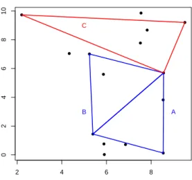
Figure 3.2: A simple example of 3 triplets labeled A, B, and C. Using the distance measure in equation 3.13, we see dist(A, B) = 0.16 while dist(A, C) = 4.21

between two tripletsA and B, we take

dist(A, B) = min

π

X

i

|ai−bπ(i)| (3.13)

whereπ(i) is a permutation of{1,2,3}. Two sets of tripletsAandB with identical lengths but different rotations, translation, and reflection would give a distance measure of zero.

Such two sets should also have the same theoretical tripletwise extremal coefficients since

the underlying field is isotropic and stationary. On the other hand, as two triangles become

more dissimilar in their respective lengths, the distance measure will increase. Thus the

clustering is based entirely on the geometry of the locations, and not on the actual estimates

of the tripletwise extremal coefficients. An example is shown in Figure 3.2

For a data set with D locations, the first step is to compute an upper triangular

dissimilarity matrix of size D₃

by D₃

which contains all distances computed using equation

(3.13). In our simulations based on D = 20 locations, we chose to group the triplets into

(48)

homogeneity and ensuring that enough triplets fall into each group to reduce variability in

group averages. Ward’s method is a hierarchical algorithm which first assigns each item to

its own cluster, and then merges two clusters chosen to minimize the overall increase in the

sum of squares (which is the sum of squared distances from each item to its cluster center).

Thus, the sum of squares begins at zero, and Ward’s method proceeds by merging items

which would result in the smallest increase. In our setting this clustering only needs to be

done once, since all of the simulated draws will be at the same locations as the observed

data. The requirement to enumerate all D₃ triplets is a practical limitation to how large

D may be. For values of D where the dissimilarity matrix is computable, it may be time

consuming to run the clustering algorithm.

The D₃triplet extremal coefficients are estimated for the observed data using equation

(2.16), and then values are averaged within the K clusters. The result is the summary of

the observed data, s = (¯θ1, ...,θ¯K). Next, we begin the approximate Bayesian computing

procedure. Independent draws from the prior φ0 ∼ π(φ) are taken. The parameter space is Φ = (0,∞) × (0,∞), except when a powered exponential is used in which case it is Φ = (0,∞)× (0,2]. For each draw from the prior, a max-stable process with unit-Fr´echet margins is simulated on the same locations and for the same number of years as

the observed data. We estimate all triplet extremal coefficients for this simulated data,

computes0 = (¯θ₁0, ...,θ¯0_K), and use the sum of the absolute deviations as the distance metric

d:

d(s, s0) =

K

X

k=1

|sk−s0k|. (3.14)

This entire process is repeated I times. The result is a collection of candidate parameter

values (φ0_i, di), i = 1, ..., I, which are then filtered as (φ0i : di 6 ). This final

filtra-tion is an independent and identically distributed collecfiltra-tion of M particles drawn from

(49)

Pos-terior standard deviations are obtained by simply regarding ρ(φ0_m) as an independent and

identically distributed collection of draws from the posterior, and empirical 95% credible

intervals can be constructed.

3.2.4 Simulation Study

We study the performance of the approximate Bayesian computing algorithm for estimating

the spatial dependence of a Schlather process with Whittle-Mat´ern correlation ρ(c1 =

1, c2, ν). Simulations were conducted in R. We specified uniform, independent priors on

[0,10] for the range c2 and smooth ν parameters. This nicely spans the range of possible

dependence functions on the spaceX (see Figure 3.3), and is consistent with the preference

for minimally informative priors. While this prior may not be the most efficient choice, it

does suffice to show the advantages of approximate Bayesian computing over the composite

likelihood approach. We make the comparison using mean square error as our measure of

performance. The simulations were all carried out for n = 100 years of data at D = 20

locations drawn from a uniform distribution on a 10 by 10 grid.

For each dataset we estimated the spatial dependence using both the composite

like-lihood approach and the approximate Bayesian computing approach shown in equation

(3.11). Figure 3.3 shows an example. Approximate Bayesian computing was done with

I = 1,000,000 draws. Due to the substantial computing time needed, we ran the

simula-tions in parallel on 50 nodes on a research computing cluster, with each node only

responsi-ble for simulating 20,000 datasets. In parallel, total computing time for one dataset in one

model was around 8 hours for the madogram method (which contains a numeric

optimiza-tion step for each iteraoptimiza-tion), but often faster for the ABC pairwise and ABC tripletwise

approaches. Given this constraint, we chose to limit the number of repetitions to only 5

replications for each model. In all there were 6 models, therefore 30 simulation runs (in

Approximate Bayesian computing for spatial extremes